An efficient nonlinear cardinal B-spline model for high tide forecasts at the Venice lagoon

This is a repository copy of

An efficient nonlinear cardinal B-spline model for high tide

forecasts at the Venice lagoon

.

White Rose Research Online URL for this paper:

http://eprints.whiterose.ac.uk/74572/

Monograph:

Wei, H.L. and Billings, S.A. (2006) An efficient nonlinear cardinal B-spline model for high

tide forecasts at the Venice lagoon. Research Report. ACSE Research Report no. 924 .

Automatic Control and Systems Engineering, University of Sheffield

[email protected] https://eprints.whiterose.ac.uk/ Reuse

Unless indicated otherwise, fulltext items are protected by copyright with all rights reserved. The copyright exception in section 29 of the Copyright, Designs and Patents Act 1988 allows the making of a single copy solely for the purpose of non-commercial research or private study within the limits of fair dealing. The publisher or other rights-holder may allow further reproduction and re-use of this version - refer to the White Rose Research Online record for this item. Where records identify the publisher as the copyright holder, users can verify any specific terms of use on the publisher’s website.

Takedown

If you consider content in White Rose Research Online to be in breach of UK law, please notify us by

An Efficient Nonlinear Cardinal B-Spline Model for High

Tide Forecasts at the Venice Lagoon

H.L. Wei and S.A. Billings

Research Report No. 924

Department of Automatic Control and Systems Engineering

The University of Sheffield

Mappin Street, Sheffield,

S1 3JD, UK

An Efficient Nonlinear Cardinal B-Spline Model for High Tide

Forecasts at the Venice Lagoon

Hua-Liang Wei and Stephen A. Billings

Department of Automatic Control and Systems Engineering, University of Sheffield Mappin Street, Sheffield, S1 3JD, UK

Abstract: An efficient class of nonlinear models, constructed using cardinal B-spline (CBS) basis functions,

are proposed for high tide forecasts at the Venice lagoon. Accurate short term predictions of high tides in the

lagoon can easily be calculated using the proposed CBS models, which can also produce good long term (up to

24 hrs ahead) forecasts for normal water levels.

Keywords: forecast, high tides, nonlinear model, B-spline, system identification, Venice lagoon.

1. Introduction

The Venice lagoon is one of the world’s most delicate and unstable ecosystems. Since the disastrous

flood that occurred in November 1966, the problems of the Venice lagoon have become one of

national and international interest. The threatened Venice city has frequently been inundated by high

waters formed in the northern Adriatic Sea, where interactions of several astronomical and

meteorological phenomena often occur. The end results are the Venice floods due to a combination of

astronomical and meteorological effects: the tides induced by the moon and the tides caused by

stormy weather arise from low atomospheric pressure combined with winds. To prevent disastrous

floods, measures have been taken since 1966, and perhaps the most famous project is the recently

endorsed MoSE (Mo

Several authors have discussed the data-based modelling problem relating to high tide forecasts at dulo Sperimentale Elettromeccanico—Experimental Electromechanical Module)

project, although the feasibility of this project is still in public debate [3][10][11]. A parallel and

complementary approach to engineering constructions, for example the barrier system as involved in

the MoSE, is to build an operational flood warning system, which is used to forecast the main surge,

for some time ahead ideally many hours or even several days. The objective of such a flood warning

system is to support some necessary actions such as the removal of goods from ground floors, the

redirection of the city boat traffic, and the installation of elevated pedestrian walkways [13]. The flood

warning system is model-based: it utilises both statistical and hydrodynamic models to obtain short

term as well as long term forecasts [13]. The hydrodynamic modelling usually starts with first

principles that require a comprehensive physical insight into the underlying dynamics of the system,

whereas the statistical modelling and similar methods often start with observational data, based on

the lagoon, by treating the regularly measured water level as a nonlinear time series, with the

assumption that no information on the hydrodynamics of the lagoon is involved, but merely observed

water level data are available [18]. Many approaches have been proposed to model the associated

nonlinear time series including nonlinear regression models, chaos and embedding methods, neural

networks, evolutionary algorithms, and other methods, see [2][18] and the references therein.

This study aims to present a novel and efficient data-based modelling approach for predicting high

tides at the Venice lagoon. In the new modelling approach, it is assumed that no a priori knowledge

about the hydrodynamics of the lagoon is available, but merely observed water level data are used.

Motivated by the successful applications of wavelet modelling frameworks, especially wavelet

multiresolution decompositions, in nonlinear time series analysis and nonlinear system identification

[1][5][6][14]-[17], cardinal B-spline multiresolution analysis (MRA) is employed in the present study

to construct parsimonious nonlinear models that can be used for high tide forecasting. As will be seen,

the resulted CBS models provide not only accurate short term forecasts, but also provide good long

term predictions for the variation of the water levels in the lagoon. Compared with existing data-based

methods, the proposed data-based CBS modelling approach can produce more accurate predictions for

high tides at the Venice lagoon.

2. Time Series Forecasting Problem

Let y t T_{t t}

0

)} (

{ ₌ be a known observed sequence for the underlying dynamical time series. The goal of

multi-step-ahead forecasts is to predict the values of y(t+s), withs≥1, using the information carried

by the observed sequence y t T_{t t}

0

)} (

{ ₌ . To achieve such a goal, a commonly used approach is to learn a

model, or a predictor, from the available data. To obtain multi-step-ahead predictions of nonlinear

time series, both iterative and direct methods can be employed [17]. In theory, long-term predictions

can be obtained from a short-term predictor, for example a one-step-ahead predictor, simply by

applying the short predictor many times in an iterative way. This is called iterative prediction. Direct

prediction, however, provides a once-completed predictor and multistep forecasts can be obtained

directly from the established predictor in a way that is similar to computing one step predictions.

Following [17], a direct approach will be considered. Take the case of the s-step-ahead forecasting

problem as an example. The task for s-step-ahead forecasts is to find a model that can predict the

value ofy(t+s) using a set of selected variables {y(t),y(t−1),, y(t−d+1)}, in the sense that

) ( )) 1 (

, ), ( ( )

(t s f( ) y t y t d e t

y + = s  − + + (1)

where f(s) with s≥1 are some nonlinear functions, e(t) is an unpredictable zero mean noise

sequence, d is the model order (the maximum lag). For a real system, the nonlinear functionf(s)is

excellent approximation capabilities, and which can represent a broad class of highly complex

systems are therefore required to ensure accurate direct s-step predictions. The model class that uses

cardinal B-splines as the basis functions to approximate the s-step predictor f(s)(⋅) satisfies all these

conditions and will therefore be investigated in the present study as a new approach of achieving

accurate direct s-step predictions.

3. Cardinal B-spline Models

3.1 Cardinal B-splines

The mth order cardinal B-spline function is defined by the following recursive formula [8]:

) 1 ( 1 ) ( 1 )

( 1 1 −

− − + −

= ₋ N ₋ x

m x m x N m x x

Nm m m , m≥2 (2)

where







∈

=

=

otherwise

x

if

x

x

N

0

)

1

,

0

[

1

)

(

)

(

1

χ

It can easily be shown that the support of the mth order B-spline function is suppNm=[0,m].

Compared with other basis functions, the most attractive and distinctive property of B-splines are that

they are compactly supported and can be analytically formulated in an explicit form. Most

importantly, they form a multiresloution analysis (MRA) [8]. B-splines are unique, among many

commonly used basis functions, because they simultaneously possess the three remarkable properties,

namely compactly supported, analytically formulated and multiresolution analysis oriented, among

many popular basis functions. These splendid properties make B-splines remarkably appropriate for

nonlinear dynamical system modelling. The most commonly used B-splines are those of orders 1 to 4,

which are shown in Table 1.

For the mth order B-spline function Nm∈L2(R) , let ( ) 2 (2 ) 2

/

, x N x k

N m j

j m

k

j = − ,

} :

{ , ∈Z

= N k

D mjk

m

j , where j,k∈Z are called the scale (or dilation) and position (translation)

parameters respectively. Following [8], for eachj∈Z, let V_jmdenote the closure of the linear span

ofDmj , namely, = < > m j L

m

j D

V clos 2_(R) . The following properties possessed by

m j

D and Vjm form the

foundations of the cardinal B-spline multiresolution analysis modelling framework for nonlinear

Table 1

Cardinal B-splines of order 1 to 4

) ( 1 x

N N2(x) 2N3(x) 6N4(x)

1

0≤x< 1 x x2 x3

2

1≤x< 0 2−x −2x2 +6x−3 −3x3+12x2−12x+4

3

2≤x< 0 0 2

) 3

(x− 3x3−24x2+60x−44

4

3≤x≤ 0 0 0 −x3+12x2 −48x+64

elsewhere 0 0 0 0

i) For any pair of integers m and j, with m≥2, the family D_jm={Nm_j,k(x):k∈Z} is a Riesz basis

of Vjm with Riesz bound A=Am (A is a constant related to m) and B=1. Furthermore, these m

bounds are optimal [8].

ii) The mth order B-spline functionN is a scaling function andm m j

V forms a multiresolution

analysis (MRA) [8].

From the above discussions, for every functionf ∈Vjm, there exists a unique sequence

) ( }

{ k∈Z∈2 Z

m k

c such that

∑

k N x k

c x

f( ) 2 /2 (2 ) (4)

For convenience of description, the symbolφwill be introduced to represent the mth order B-spline

functionN and the symbol ‘m’ will be omitted in associated formulas. m

3.2 The Cardinal B-spline Model for High Dimensional Problems

The result for the 1-D case described above can be extended to high dimensions and several

approaches have been proposed for such an extension. Tensor product and radial construction are two

commonly used methods [5][15][16]. In the present study, a linear additive CBS model structure will

be employed to represent a high dimensional nonlinear function.

For a d-dimensional function f∈L2(Rd), the linear additive representation is given below

) ( ) ( ) ( ) , , ,

(x₁ x₂ x_d f₁ x₁ f₂ x₂ f_d x_d

f  = + ++ (5)

where fr∈L2(R) (r=1,2, …, d) are univariate functions, which can be expressed using the expansion

(4) as below

∑

r x c x

f ( ) , φ, ( ) (6)

where , (x) 2 /2 (2 x k)

j j k

j = φ −

Now consider the model given by (1) and let x_r(t)=y(t−r+1)for r=1,2, …, d. Using (5) and

(6), model (1) can be expressed as

∑

f s t y 1 ) ( )) ( ( ) (

∑∑

j x t

c 1 , ) , ( , ( ( )) Z

φ +e(t) (7)

The remaining task is how to deduce, from (7), a parsimonious model that can be used for

s-step-ahead forecasts for a given prediction horizon s. The following problem needs to be solved:

• How to choose the scale and position parameters j and k ?

• In practical modelling problems, the variables xr(t) (r=1,2, …, d), as the lagged versions of

) (k

y , are usually sparsely distributed in the associated space and therefore the problem may be

ill-posed. The representation (7) is thus often redundant in the sense that most of the basis

functions (or model terms),φ_j,k(⋅)in (7), can be removed from the model, and experience shows

that only a small number of significant model terms are required for most nonlinear dynamical

modelling problems. The question is: how to select the potential significant model terms from a

large number of candidate basis functions?

The scale and position determination problem will be discussed in the following section. The model

term selection problem has been systematically investigated in [4][7]. In the present study, the

orthogonal forward regression (OFR) algorithm [4], coupled with a Bayesian information criterion

(BIC) [9][12], will be used to select significant model terms and to determine the model size (the

number of model terms included in the final model).

3.3 Determination of the scale and position parameters

Assume that a d-variate function f of interest is defined in the unit hypercube[0,1]d. Consider the scale

parameter determination problem first. Experience on numerous simulation studies relating to wavelet

multiresolution modelling for dynamical nonlinear systems, see for example, [5][15][16] and the

references therein, has shown that the scale parameter j in model (7) should not be chosen too large. A

value that is between zero and two or three for j is often adequate for most nonlinear dynamical

modelling problems.

For cardinal B-spline functions, the position parameter k is dependent on the corresponding

resolution scale j. Indeed, for each fixed pointx∈[0,1], since N has compact support, all except a _m

finite number of terms in the expansion (4) are zero. Take the 4th-order B-spline function as an

example. At a given scale j, the non-zero terms are determined by the position parameter k for

1 2 , , 1 , 2 ,

3− − −

−

= j

support for the associated function , (x) 2 /2(2 x k)

j j k

j = −

φ is [2−jk, 2−j(m+k)], therefore, the

position parameter k at a resolution scale j should be chosen as −(m−1)≤k≤2j−1.

4. Water Level Modelling and High Tide Forecasting

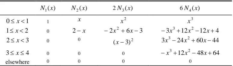
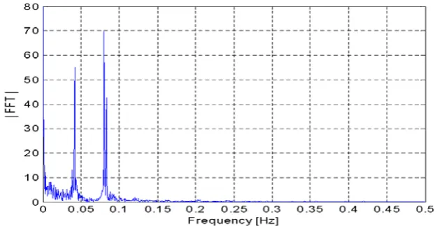
4.1 The Data

The data set used here is formed by the hourly recorded observations of water levels at Punta della

Salute, Venice Lagoon, for the period from January 1990 to December 1994. Only 2208 data points,

corresponding to the water levels of the period from October to December 1990, were used for model

training, and the remaining data were used to test the performance of the identified model. The

associated Fourier spectrum, estimated via fast Fourier transform, and the power spectral density

(PSD), estimated via the Welch method, are shown in figures 1 and 2, where the two dominant

frequencies are calculated to be f =0.0417 Hz and₁ f =0.0808 Hz, which correspond to the two main ₂

oscillation cycles of T1=1/f1≈24hrs and T2=1/ f2 ≈12hrs, respectively.

Using the information given by figures 1 and 2, the maximum lag for the input variables in the

initial modelling procedure was chosen to be 24, to cover the range of the maximum oscillation cycle.

Thus, the variables y(t),y(t−1),,y(t−23)were used as inputs to form a predictor, whose output

was the future behaviour, denoted byy(t+s) (s≥1).

Note that the original data were initially normalized to [0,1] via a transform

) /( ) ) ( ~ ( )

(t y t a b a

y = − − , where ~ ty( )indicate the initial observations, anda=−100and b=150. The

identification procedure was therefore performed using normalized values y(t). The outputs of an

identified model were then recovered to the original measurement space by taking the associated

inverse transform.

4.2 The Models

Let xr(t)=y(t−r+1), r=1, 2,…, 24. The structure of the initial CBS model was chosen to be

) (t s

y +

∑ ∑

= =− = 24 1 0 3 , 0 ) , ( ,

0 ( ( ))

r k

r k r s

k x t

c φ

∑ ∑

= =− + 24 1 1 3 , 1 ) , ( ,

1 ( ( ))

r k

r k r s

k φ x t

α (8)

whereφ_j,k(x)=2j/2φ(2jx−k),withj,k∈Z, are the 4th-order B-spline functions. Notice that model

(8), which involves two scale levels for j=0 and j=1, is in structure different from model (7), where

the model termφ_j,k(⋅) only involves a single scale level. The reason that the initial model (8) was

chosen to be such a structure was to enrich the pool of the model term dictionary, so that basis

functions with different scale parameters can be sufficiently utilised. Although a total number of 216

model terms (basis functions) were involved in the initial model (8) for any given s, only a small

number of basis functions were required to describe the relationship between

)} 23 ( , ), 1 ( ), (

{y t y t−  y t− and y(t+s), and significant model terms were efficiently selected by

performing a model term detection algorithm,. Also, different values for s usually led to different final

models. For each s, a Bayesian information criterion (BIC) [9][12] was used to determine the number

of model terms, and the parameters of the final CBS model was then re-estimated by introducing a

linear moving average (MA) model of order 10 [5][17].

4.3 Prediction Results

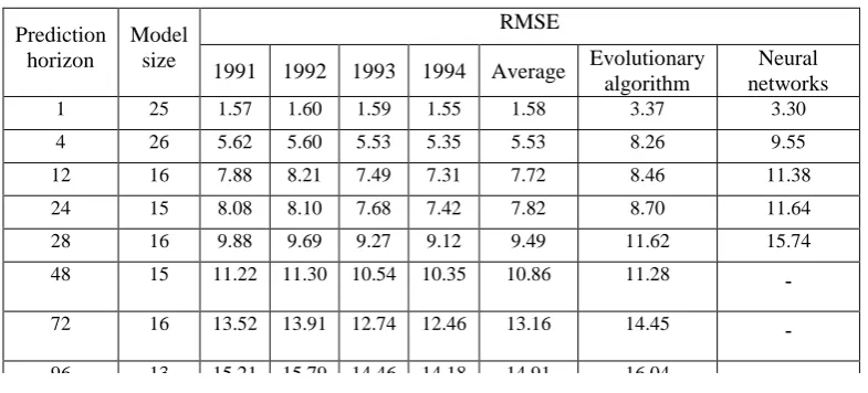
For convenience of comparison with other results in [2][18], eight cases, corresponding to s=1, 4, 12,

24, 28, 48, 72, and 96, were considered, and eight different CBS models were identified. The resultant

Table 2

Prediction errors for the water level of the years 1991, 1992, 1993, and 1994, with 8760, 8760, 8784, and 8760 records, respectively.

Prediction horizon

Model size

RMSE

1991 1992 1993 1994 Average Evolutionary algorithm

Neural networks

1 25 1.57 1.60 1.59 1.55 1.58 3.37 3.30 4 26 5.62 5.60 5.53 5.35 5.53 8.26 9.55 12 16 7.88 8.21 7.49 7.31 7.72 8.46 11.38 24 15 8.08 8.10 7.68 7.42 7.82 8.70 11.64 28 16 9.88 9.69 9.27 9.12 9.49 11.62 15.74 48 15 11.22 11.30 10.54 10.35 10.86 11.28

72 16 13.52 13.91 12.74 12.46 13.16 14.45 96 13 15 21 15 79 14 46 14 18 14 91 16 04

eight models were applied respectively over four test data sets, for the years from 1991 to 1994, to

calculate s-step-ahead forecasts of the water levels. Prediction performance, measured by the

root-mean-square-errors (RMSE) as used in [2][18], over the four test data sets, obtained from the

identified CBS models, are shown in Table 2, where some results produced from multilayer neural

networks [18] and evolutionary algorithms [2] are also listed to facilitate the comparison. Clearly,

compared with the results produced by multilayer neural networks [18] and evolutionary algorithms

[2], where over 45,000 observations were involved in the training data set, the results produced by the

proposed CBS models are better, both for short and long term forecasting.

To visually illustrate the CBS models’ performance for high tide forecasting, short term

predictions for some abnormal high tides, and medium and long term predictions for some normal

high tides, were calculated using the identified CBS models. Figure 3 presents the one-step-ahead

(one-hour-ahead) prediction for typical abnormal high tides, figures 4 and 5 presents 4 and

12-step-ahead predictions for typical high tides, while figures 6 and 7 present 24 and 48-step-12-step-ahead

predictions for typical normal water level at the Venice lagoon.

5. Conclusions

The CBS models are a class of nonlinear representation, where dilated and translated versions of

cardinal B-spline functions were chosen to be the basis functions (regressors or model terms). As a

special class of linear-in-the-parameters representation, the CBS models are easy to train using some

standard model term selection algorithms, and the final identified models usually only include a small

number of significant model terms. The proposed CBS models provide an efficient representation for

tide forecasts at the Venice lagoon: the resulting models can produce accurate short term predictions

for typical abnormal high tides; can produce good predictions for typical high tides; and can produce

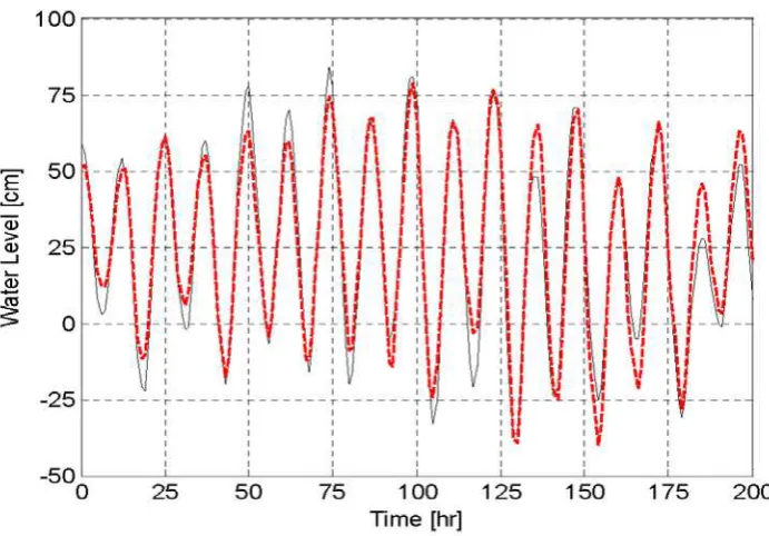
Fig. 3 One-hour-ahead prediction for typical abnormal high tides. The thin line with dots indicates the measurements (observed in 1992), and the thick line with circles indicates the prediction values.

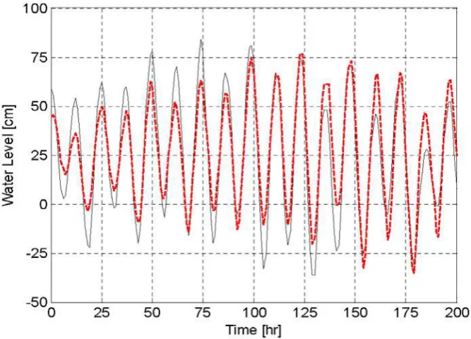
Fig. 5 Twelve-hour-ahead prediction for typical high tides. The thin solid line indicates the measurements (observed in 1993), and the thick dashed line indicates the prediction values.

Fig. 7 Forty-eight-hour-ahead prediction for typical normal water level. The thin solid line indicates the measurements (observed in 1994), and the thick dashed line indicates the prediction values.

Acknowledgements

The authors gratefully acknowledge that this work was supported by EPSRC (UK).

References

[1] Allingham, D., West, M. and Mees, A. (1998). Wavelet reconstruction of nonlinear dynamics. International

Journal of Bifurcation and Chaos, 8(11), 2191-2201.

[2] C. L. del Arco-Calderon, P. I. Vinuela, and J. C. H. Castro, “Forecasting time series by means of

evolutionary algorithms,” Lecture Notes in Computer Science, 3242, pp.1061-1070, 2004.

[3] BBC News, “Venice launches anti-flood project,” May 14, 2003. Online:

[4] S. A. Billings, S. Chen, and M. J. Korenberg, “Identification of MIMO non-linear systems suing a forward

regression orthogonal estimator,” International Journal of Control, 49(6), pp. 2157-2189, 1989.

[5] S. A. Billings and H. L. Wei, “A new class of wavelet networks for nonlinear system identification,” IEEE

Transactions on Neural Networks, 16(4), pp. 862-874, 2005.

[6] L. Y. Cao, Y. G. Hong, H. P. Fang, and G. W. He, “Predicting chaotic time series with wavelet networks,”

Physica D, 85(1-2), pp. 225-238, 1995.

[7] S. Chen, S. A. Billings, and W. Luo, “Orthogonal least squares methods and their application to non-linear

system identification,” International Journal of Control, 50(5), pp. 1873-1896, 1989.

[8] C. K. Chui, An Introduction to Wavelets. Boston: Academic Press, 1992.

[10] E. Rosenthal, “Venice turns to future to rescue its past,” The New York Times Electronic Edition, Feb. 22,

2005. Online:

[11] E. Salzano, “The Venice Lagoon: what it is, what they are doing on it,” Eddyburg, Aug. 2005. Online:

[12] G. Schwarz, “ Estimating the dimension of a model,” Ann. Stat., 6(2), pp. 461-464, 1978.

[13] J. Vieira, J. Fons, and G. Cecconi, “Statistical and hydrodynamic models for the operational forecasting of

floods in the Venice Lagoon,” Coastal Engineering, 21(4), pp. 301-331, Dec. 1993.

[14] H. L. Wei, S. A. Billings, and M. Balikhin, “Analysis of the geomagnetic activity of the D-st index and

self-affine fractals using wavelet transforms,” Nonlinear Processes in Geophysics, 11(3), pp.303-312,

2004a.

[15] H. L. Wei, S. A. Billings, and M. A. Balikhin, “Prediction of the Dst index using multiresolution wavelet

models,” Journal of Geophysical Research, 109(A7), A07212, doi:10.1029/2003JA010332, 2004b.

[16] H. L. Wei and S. A. Billings, “Identification and reconstruction of chaotic systems using multiresolution

wavelet decompositions,” International Journal of Systems Science, 35(9), pp. 511-526, 2004c.

[17] H. L. Wei and S. A. Billings, “Long term prediction of nonlinear time series using multiresolution wavelet

models,” International Journal of Control, 79(6), pp. 569-580, 2006.

[18] J. M. Zaldivar, E. Gutiérrez, I. M. Galván, F. Strozzi, and A. Tomasin, “Forecasting high waters at Venice

Lagoon using chaotic time series analysis and nonlinear neural networks,” Journal of Hydroinformatics,