Network Effect in Geocentre Motion

(1)

Network Effect in Geocentre Motion

Umma Jamila Zannat

February 2019

A thesis submitted for the degree of Doctor of Philosophy of The Australian National University

(2)

(3)

Statement of Originality

The work contained in this thesis is my own original research. No part of it has been submitted, or is being submitted, for any other degree. To the best of my knowledge, all sources used and any guidance received in preparation of this thesis have been duly acknowledged.

(4)

(5)

Acknowledgements

First of all, I would like to express my gratitude to my supervisory panel. I am grateful to Dr. Paul Tregoning for giving me the opportunity to study under his supervision, for navigating me through the daze of postgraduate research, and for believing in me. I also thank Dr. Simon McClusky, Dr. Achraf Koulali, and Dr. Herb McQueen for their constant support, help and guidance. It was a pleasure and an honour working with the team for the past few years.

I would also like to thank the administrative team here at the ANU for their enthusiastic support. Especially, I am indebted to Maree Coldrick for always being there for me. I also sincerely thank Jochen Brocks for his moral support during a difficult time for me.

My immensely enjoyable time at the Research School of Earth Sciences was a gift from my fellow students and colleagues that I will cherish forever. I am grateful for the friendship of Sebastian Allgeyer, Evan Gowan, Siyuan Tian, Veronika Emetc, Bianca Kallenberg, Salim Masoumi, and Michael Moore. I would turn to Anthony Purcell whenever I needed help with my mathematics, and I was also fortunate enough to attend a statistics course by Malcolm Sambridge that was instrumental to this work.

(6)

(7)

Abstract

Geocentre motion is the motion of the centre of mass of the Earth system with respect to the geometric centre of figure of the solid Earth surface because of the continual deformation of the Earth by geophysical processes. This motion is important both in theory and in practice to understand and interpret various mass transport phenomena and their consequences, such as sea level rise, postseismic relaxation, polar ice melting, and glacial isostatic adjustment.

Global reference frames for space geodetic point positioning are realised using measurements of the relative motion between satellites orbiting around the centre of mass on one hand and stations placed on the Earth’s surface on the other. Therefore, reliable modelling of the geocentre motion is vital for the stability and the accuracy of these reference frames. In turn, the interpretation of many geodynamical quantities of current interest, such as the mean sea level, depends heavily on the quality of the adopted reference frame.

Space geodetic measurement of the true geocentre motion, however, is difficult due to the discrete and therefore incomplete sampling of the Earth’s surface by geodetic stations. In other words, there is a discrepancy between the centre of figure of the Earth surface and the centre of network of the stations, called the network effect, arising from the sampling bias of the geodetic network.

(8)

scales as 1/ N, and we provide an explicit formula for this estimate in terms of the vector spherical harmonics expansion of the displacement field.

We assess the effectiveness of the expected bias as an estimate of the net-work effect by simulating the displacement fields for two illustrative geodynamical processes: (instantaneous) coseismic deformation due to great earthquakes, and (time-dependent) elastic deformation due to surface water movements. We ac-cordingly concentrate on the instantaneous changes and the secular drifts in the Helmert parameters for the two cases respectively.

We found that, in both case studies, the network effect is often as large as the changes in the Helmert parameters themselves. Hence, current space geodetic networks are indeed inadequate for verifying the geocentre motion predictions by geophysical models accurately. Nevertheless, our simulations validate the expected bias to be a reasonable estimate of the network effect.

(9)

List of Publications

The bulk of the original research is contained in Chapters3,4and5. These results have been reported in:

Zannat, U. J., and P. Tregoning (2017a), Estimating network effect in geo-center motion: Theory,Journal of Geophysical Research: Solid Earth,122,doi: 10.1002/2017JB014246

(14)

(15)

List of Figures

1.1 Geocentric coordinate systems: Cartesian and spherical . . . 3

1.2 East component of the position timeseries of GPS station SAMP . . . 12

1.3 Vertical component of the position timeseries of GPS station BRAZ . . . 14

1.4 Schematic diagram of the network polyhedron in inertial space . . . 16

1.5 The degree-1spherical harmonics . . . 17

2.1 Schematic diagram of geocentre motion due to surface deformation . . 25

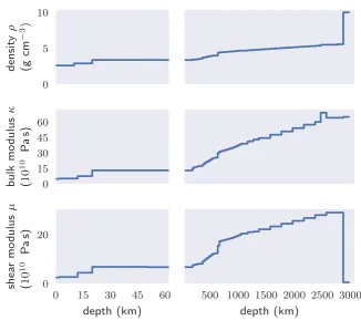
2.2 The physical properties of the Preliminary Reference Earth Model . . . 48

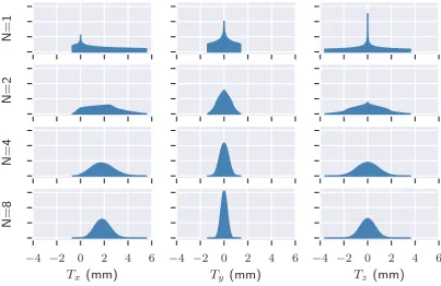
3.1 Distributions of the components ofTCN from the degree-1modes . . . . 66

3.2 The dependence of the expected bias on the network sizeN . . . 68

3.3 Voronoi decomposition of the surface of the sphere . . . 71

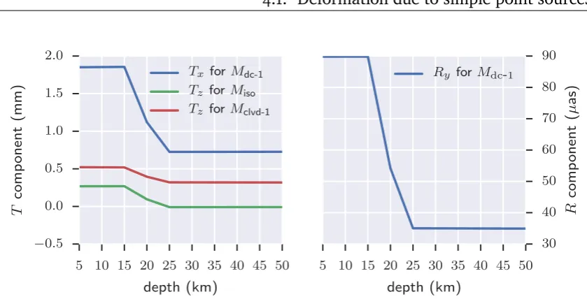
4.1 Seismic source depth dependence of the CF parameters . . . 77

4.2 Seismic source depth dependence of expected bias in CN parameters . . 81

4.3 Comparison between the summation and transformation methods . . . 84

4.4 Horizontal coseismic offsets for the two great earthquakes . . . 85

4.5 Geographical distribution of the three example networks . . . 86

4.6 Effect of exclusion of an epicentral cap on GC motion . . . 92

4.7 Summation and transformation method with epicentral cap excluded . 93

5.1 Geocentre motion caused by hydrological loading deformations . . . 99

5.2 Network effect in secular velocity due to surface water movements. . . 100

6.1 Comparison ofnerfwith half-space theory in the near field . . . 108

(16)

(17)

List of Tables

4.1 Statistics of the displacement field due to the point sourceM_iso . . . 79

4.2 Statistics of the displacement field due to the point sourceM_dc-1 . . . 79

4.3 Statistics of the displacement field due to the point source M_dc-2 . . . 80

4.4 Statistics of the displacement field due to the point source M_clvd-1 . . . . 80

4.5 Shifts in instantaneous CN parameters (SA event, SOPAC network). . . 88

4.6 Shifts in instantaneous CN parameters (TO event, SOPAC network) . . 89

4.7 Shifts in instantaneous CN parameters (SA event, ITRF core networks) 90

4.8 Shifts in instantaneous CN parameters (TO event, ITRF core networks) . 91

4.9 Shifts in instantaneous CWN parameters (SA event) . . . 95

4.10 Shifts in instantaneous CWN parameters (TO event) . . . 96

5.1 Shifts in the derivative CN and CWN parameters (SOPAC network). . . 102

(18)

(19)

List of Abbreviations

CE Centre of solid Earth

CF Centre of Figure

CLT Central Limit Theorem

CMB Core-Mantle Boundary

CM Centre of Mass

CMT Centroid Moment Tensor

CN Centre of Network

CSR Center of Space Research

CWN Centre of Weighted Network

DORIS Doppler Orbitography and Radiopositioning Integrated by Satellite

ECCO Estimating the Circulation and Climate of the Ocean

ECEF Earth Centred, Earth Fixed

EOP Earth Orientation Parameter

GC Geocentre

GCMT Global CMT Project

GGM03 GRACE Gravity Model 03

GGRF Global Geodetic Reference Frame

GIA Glacial Isostatic Adjustment

GNSS Global Navigation Satellite Systems

GOCE Gravity Field and Steady-State Ocean Circulation Explorer

GPS Global Positioning System

GRACE Gravity Recovery and Climate Experiment

GSM GRACE Satellite-only Model

HP Helmert Parameter

(20)

ICRF International Celestial Reference Frame

ITRF International Terrestrial Reference Frame

JPL Jet Propulsion Laboratory

LLN Law of Large Numbers

LOD Length Of the Day

MSL Mean Sea Level

NE Network Effect

NNR No-Net-Rotation

OMCT Ocean Model for Circulation and Tides

OM Ocean Model

PDMT Present-Day surface Mass Trend

PODAAC Physical Oceanography Distributed Active Archive Center

PREM Preliminary Reference Earth Model

PSR Post-Seismic Relaxation

RF Reference Frame

RL05 Release-05

SA Sumatra–Andaman

SLR Satellite Laser Ranging

SOPAC Scripps Orbit and Permanent Array Center

TO T¯ohoku–Oki

TRF Terrestrial Reference Frame

TRS Terrestrial Reference System

USGS United States Geological Survey

(21)

(22)

(23)

Chapter 1 Introduction

It has been over half a century since we started sending artificial satellites into orbit around the Earth. These satellites have enabled exciting new technologies that revolutionised not only communication and navigation, but also the venerable science of geodesy. Today, with the help of a constellation of space geodetic satellites, we can monitor the geodynamical processes sculpting the Earth crust in near real-time.

These processes vary widely in their characteristic timescales. On one hand, oceanic and atmospheric tides deform the surface of the Earth on a subdaily basis. However, the mostly periodic motions they induce generally have much smaller drift components at larger timescales. On the other hand, in a few thousand years the viscoelastic response of the Earth to earthquakes and climate change becomes significant, Earth surface area is created and destroyed in volcanic activity and tectonic motion, and redistribution of mass on and inside the Earth crust changes the length of the day, to name just a few. Needless to say, modelling and predicting the shape of the Earth accurately over such a long period, if attempted, would be a truly formidable task.

(24)

we will also assume that the influence of lower-frequency processes are already included in the secular motion during our period of interest.

Most importantly for this thesis, the overall motion of the crust, called the geo-centre motion, due to these disruptions is only partially captured by the movements of the geodetic stations on Earth. That is, it is quite probable that due to the uneven geographical distribution of the stations, the average movement recorded by the stations will differ considerably from the true geocentre motion. This difference, called the “network effect”, has implications for the realisation of global terrestrial reference frames from the position timeseries of these stations.

Our principle contribution in this thesis is a method to estimate the magnitude of the network effect. We will see that generally we expect the network effect to decrease when the number of stations on the Earth surface is increased. However, for the currently active network of geodetic stations around the world, we will also show that in some cases of interest the network effect may be as large in magnitude as the geocentre motion itself. Hence, the problem posed by the network effect persists in these cases even with the unprecedented coverage we have today. Consequently, it will have to be carefully addressed if we are to reconcile the geocentre motion predicted by geophysical theories with their space geodetic measurements at the millimetre (mm) level.

1.1 Space geodesy and the ITRF

One of the principal tasks of geodesy, measuring point positions and velocities on the Earth surface, requires a reference frame (RF) to enable us to report and interpret geospatial data. The RF establishes a one-to-one correspondence between points in space, which are physical, and their designated coordinates, which are numbers can be stored in a disk, processed by a computer, and transmitted over the Internet. A geodetic measurement site, in effect, acts as a label on one of the mass elements forming the Earth whose idealised motion as a point particle in space can then be described by its time-dependent coordinates.

(25)

1.1. Space geodesy and the ITRF

z

x

equator

prime meridian

θ

P

ϕ

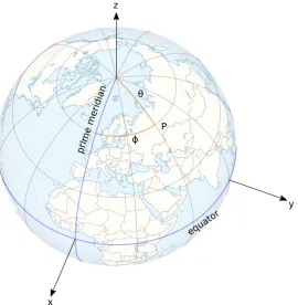
[image:25.595.198.469.160.437.2]

y

Figure 1.1: Geocentric coordinate systems for a spherical Earth: Cartesian and spherical. The angular coordinatesθ andφ are the co-latitude and the longitude, respectively, of the point P. See AppendixA for our conventions.

natural to set up our coordinate system with the origin at its centre and to locate the points on the surface using angular coordinates (Figure 1.1). Our RF would then also rotate uniformly with the Earth around its axis. It would then enable us to assign reference coordinates to known locations, or stations, and to follow their motion in time as deviations from their reference positions. Even though our Earth is slightly ellipsoidal in reality, we continue to follow this program, making appropriate modifications to the concepts when necessary.

(26)

of the Earth as a point particle, known as the Centre of Mass (CM) of the Earth system (solid Earth, oceans and atmosphere), moves under the influence of the Sun and other celestial objects, but is unaffected by processes internal to Earth. If we model and thereby remove the external influences from consideration, which we will assume to have been done already from now on, the CM moves at a constant velocity in a straight line through inertial space.

It is not difficult to show that the CM is not affected by internal geodynamical processes. For notational simplicity, consider the Earth to be a collection ofN point particles where thekth particle has mass m_k and positionr_k with respect to some inertial reference frame. Then the CM of the system is defined to be:

rCM= P

kmkrk P

kmk

(1.1)

Also, let the force that the jth particle exerts on the kth particle be denoted by F_jk, so that the total force on thekth particle isP_jF_jk, and by Newton’s third law, F_jk=−F_{k j}. Differentiating Equation1.1twice with respect to time gives,

d2

d t2rCM= P

kmk d2 d t2r_k

P kmk

= P

j,kFjk P

kmk

=0 (1.2)

since opposing forces occur in pairs in the sum in the numerator. Thus the velocity of the CM is constant.

Since the CM moves uniformly with respect to some inertial RF, a non-rotating RF with the CM at the origin is itself inertial. A primary advantage of an inertial RF is that the laws of physics, such as the conservation of momentum, angular momentum, and energy, hold with respect to it. Note, however, that in reality the terrestrial frame rotates with the Earth and therefore is non-inertial. We sometimes refer to this rotating frame as the “Earth Centred, Earth Fixed” (ECEF) frame.

(27)

1.1. Space geodesy and the ITRF

diverse Earth science applications. It is designed to draw from the strengths of the individual techniques, and to be reproducible, stable, accurate and accessible to the research communities worldwide. Its state-of-the-art accuracy and precision are maintained by the geodetic community by continual improvements to its mea-surements and methodology. For overviews of the infrastructure around the ITRF, see, for example,Plag and Pearlman [2009] andAltamimi and Collilieux[2013].

For its realisation, the ITRF uses combined measurements and observations from four space geodetic techniques: Satellite Laser Ranging (SLR), Very-Long-Baseline Interferometry (VLBI), Doppler Orbitography and Radiopositioning Integrated by Satellite (DORIS), and Global Navigation Satellite Systems (GNSS) such as the Global Positioning System (GPS). The unique characteristics of the different geode-tic techniques are advantageous for measuring different ITRF parameters.

The ITRF takes its origin to be the time average of the SLR realisation of the CM over several decades of observations. SLR satellites here have the advantage of a mostly spherical design that enables their orbits to be modelled precisely over weeks. The orbit modelling for GPS is relatively less accurate since its satellites are subject to more complex non-gravitational forces due to their complex geometry [Blewitt et al., 2010]. The spatio-temporal coverage of the Earth surface by GPS, on the other hand, is much denser. Moreover, GNSS binds the different techniques together through co-location ties between stations of different techniques at the same location [Altamimi et al.,2011].

Since the space geodetic techniques employ several different methods to measure distances for positioning by trilateration, the ITRF also considers scale transforma-tions between the RFs. The ITRF scale parameter is obtained by taking the average of the scale parameters of the SLR and the VLBI frames through stacking their observations togetherAltamimi et al.[2016].

(28)

DORIS has the most homogeneous station distribution but contributes less to the spatial resolution. GNSS, DORIS and SLR are used together in the ITRF to position the orbiting satellites.

1.2 Relevance of the ITRF to geophysical research

Earth observations from space have become integral to diverse aspects of our life ranging from weather forecast to public policy. Because of their global coverage and low latency, they provide us with vital, and potentially life-saving, timely information on meteorological and geological hazards such as cyclones, floods, earthquakes, volcano eruptions, wildfires, tsunamis, landslides, and subsidence.

Naturally, satellite observations also serve as invaluable sources of primary data to geophysics and geodesy. They have been instrumental to our evolving under-standing of the complex interactions between the lithosphere, the hydrosphere, the cryosphere, and the atmosphere, as well as the mantle and the core. Space observations also provide critical validation, justification and constraints for the geodynamical models that codify this understanding.

Terrestrial RFs, however, are especially relevant to the analysis of global trends in mass transport processes over timespans of decades or even centuries. Unfortunately, the signals indicative of these trends are often embedded in much larger local variations (such as local hydrological loading). Moreover, these signals are, more often than not, of the order of parts-per-billion (ppb) when compared to the planetary scale. Understandably, satisfactory quantification of such tiny effects require staggeringly high quality measurements. Currently one of the principal factors limiting further understanding of phenomena such as mean sea level (MSL) rise, plate tectonics, anthropogenic land subsidence, present-day surface mass trend (PDMT), or polar ice melting is the uncertainty in the realisation of the RF itself, thanks to the impressive accuracy and resolution of modern satellite techniques [Blewitt et al.,2010;Wu et al.,2011].

(29)

phe-1.2. Relevance of the ITRF to geophysical research

nomena, it is imperative to realise a global terrestrial RF of the highest accuracy, precision and stability presently achievable. The ITRF is the embodiment of just such a concerted international effort.

Consider, as an example, the case of global sea level rise. Reliable and com-prehensive historical records of sea level changes over the last century have been derived from measurements by tide gauges. Traditionally, a tide gauge measures the relative vertical movements of the ocean surface with respect to a horizontal reference level fixed to the land. The problem here, of course, is that for a mostly spherical planet like ours, the notion of a flat horizontal reference plane is only local, and cannot be extended to cover the whole planet so as to obtain a global measure of sea level change. It is more appropriate, in the global case, to measure the height of the sea surface from some fixed point at the planet’s centre, which we may conveniently pick to be the origin of a geocentric reference system. Unfortunately, the interpretation of the mean sea level (MSL), and therefore, the MSL change, has now become inextricably tied to the choice of that reference frame, and our ability to realise it in practice [Kovalevsky et al.,2012]. On the other hand, provided that we express all our observations in this frame, we can now collate and compare measurements from various sources, including those from space geodesy.

The MSL rise is especially interesting in that its determination involves all the “three pillars of geodesy” [Rummel et al.,2005]:

geometry of the solid Earth, including ocean bottom, serves as a reference for measuring relative sea level changes

orientation of the Earth with respect to the celestial frame changes as a result of mass exchange between the oceans and the polar ice caps

gravity field due to the mass distribution of the Earth determines the shape of the geoid that the sea surface follows in static equilibrium

(30)

have a significant effect on the measurement of MSL [see, for example, Beckley et al.,2007].

The ITRF thus provides a framework to connect and to combine the observational data and their analysis from different regions, different missions, different methods, and different decades consistently and meaningfully. Currently, the estimated uncertainty of the ITRF2014 origin is less than3mm and that of the origin velocity is less than 0.2 mm per year (yr) [Altamimi et al., 2016]. For comparison, the resolutions of the altimetry- and gravimetry-based observations of sea level are also around that level [Blewitt et al., 2010]. Clearly, the uncertainty in the RF realisation presents us with a road-block, among others, towards improving our measurements of changes in MSL. Incidentally, the precision of GPS measurements of point position of the sites stationed on the solid crust is believed to be much better at∼1mm, whereas the precision of the velocity is∼1mm/yr.

Using terrestrial as well as space measurements of sea level, Collilieux and Wöppelmann [2011] calculated the average MSL rise over the past century to be ∼1.6 mm/yr, for instance. Their analysis there also show that the uncertainty in the scale rate of the ITRF, currently estimated to be equivalent to 0.1 mm/yr, propagates directly into this estimate. In addition, up to50%of the origin velocity uncertainty, currently estimated to be0.2mm/yr, also makes it into the uncertainty in the final result, depending on the network geometry. Note, however, that these recent uncertainty estimates are not too far from the requirement inBlewitt et al. [2010] of frame stability of0.1mm/yr and scale stability of the equivalent of0.05 mm/yr spanning decades for reliable MSL change observations, owing to the rapid increase of accuracy of geodetic RFs by roughly an order of magnitude per decade since their introduction.

Besides, improving the stability of the ITRF is also important for providing tighter observational constraints and stricter validation for global climate models that predict MSL change. Additionally, the high quality and stability of the ITRF facilitates the identification and separation of different geophysical phenomena si-multaneously at work. Its fields of practical applications include surveying, national geodetic datum definition, satellite navigation, and measurement of satellite orbits.

(31)

1.3. Realisation of the ITRF

a resolution on the Global Geodetic Reference Frame (GGRF) for Sustainable Development1encouraging its adoption.

1.3 Realisation of the ITRF

It is sometimes useful to maintain a distinction between a terrestrial reference system (TRS) on one hand and a terrestrial reference frame (TRF) on the other. The TRS is an idealisation: a theoretical and mathematical construct that comprises of conventions for the origin and the orientation, physical units and constants, geodetic datum, and self-consistent modelling of the Earth’s shape, rotation, and gravity [Blewitt et al.,2010]. The TRF, however, is a concrete realisation of the TRS, specified by assigning position and velocity coordinates at a reference epoch to a set of globally distributed reference marks on the solid Earth’s surface.

In practice, because of ongoing theoretical, methodological, and technological improvements, these assignments get upgraded with each new incarnation of the ITRF. There have been twelve such incarnations so far, starting from ITRF88 to the present ITRF2014. Considerable care is taken to ensure that discontinuities in the frame origin and alignment at the transition from one version to the next are as limited as possible.

The ITRF is currently derived from the station position timeseries of a global network of reference geodetic sites that nevertheless show non-linear motion from various loading phenomena or instrumental changes [see, for example,Bevis and Brown, 2014]. From a slightly different perspective, the presumed (piecewise) linearity of the station position timeseries in the realisation of the ITRF is, in reality, the result of the linearisation of a more general non-linear estimation problem [Dermanis,2004].

In addition, the ITRF also relates the orientation parameters of the RF to polar motion and universal time EOPs in order to connect to the ICRF. Initially, the ITRF2000 adopted the no-net-rotation (NNR) condition for the orientation time evolution of the Earth’s tectonic plates using the NNR-NUVEL-1A plate model [Argus and Gordon,1991]. This entails aligning the RF with the so-called Tisserand frame that minimises the kinetic energy of the lithosphere and, as a consequence, the total

(32)

angular momentum of the crust in this RF becomes zero. Successive ITRF versions continued to inherit this alignment of the RF from their predecessors [Altamimi et al.,2012].

Nevertheless, note that the RF parameters themselves are being defined only indirectly through the coordinates of geodetic sites, and thus the measurement of the point positions of the reference sites and the realisation of the RF are closely intertwined. Mathematically, RF realisation is a vastly over-specified problem that in general admits no exact solutions, only approximate ones. The number of unknown RF parameters here is only 14: 3 origin components, 1 scale factor, 3 orientation parameters, and their corresponding 7 time derivatives. In contrast, each of the more than a thousand reference sites contribute 6 equations, 3 for the position and 3 for the velocity components, at each epoch of observation for these parameters.

1.4 Impact of geophysical processes on the ITRF

The non-linear motion of the ground stations is caused by a complicated network of processes: tidal displacements, atmospheric loading, hydrological mass movements, earthquakes, plate tectonics, and even internal mass movements. Since the satellite observations of station positions are not fully compatible with the simple linear trajectory model that the ITRF realisation hypothesises, the RF realised from the reference sites in general undergoes what is referred to as RF deformation as a result of this motion. The resulting internal geometric inconsistency, in turn, damages the accuracy of positioning of the non-reference geodetic sites as well. Imperfections in our modelling of satellite orbits or satellite signal propagation also contribute to this inconsistency.

We discuss here two geodynamical processes whose consequences can be ob-served from space: coseismic deformation due to great earthquakes with moment magnitude M_W _≥ 8.0 and elastic deformation due to surface water loading. In Chapters 4 and 5 respectively, they will serve as two qualitatively different case studies for the methods of estimating the network effect that we will introduce in Chapter3.

(33)

1.4. Impact of geophysical processes on the ITRF

frame. Still, the impact of imperfections in our modelling of crustal deformation, satellite orbits, or satellite signal propagation on the ITRF continues to be the focus of active research. In fact, Altamimi et al. [2016] found that published geophysical models of crustal deformations, especially for postseismic relaxation, are unavailable in many cases, and are difficult to assess for quality for the purposes of RF construction in general, and settled for fitting parametric models to the observed timeseries instead.

1.4.1 Great earthquakes

Significant earthquakes leave their marks on the face of the Earth. Naturally, the elastic as well as the viscoelastic deformations of the Earth due to earthquakes have been the subject of studies for decades. Since, in general, the surface displacement gradually diminishes with distance from the epicentre, the far field signature of an earthquake is difficult to detect. However, great earthquakes like the Sumatra– Andaman earthquake in December 2004 or the T¯ohoku–Oki earthquake in March 2011 are violent enough for the deformation to occur not only near the earthquake but all over the world. Again, thanks to the incredible resolution of modern space geodetic observation and analysis, it is now possible to measure this far field offset, despite it being in the mm order, systematically across the globe.

Great earthquakes are generally defined to be those with M_W ≥8.0 and are somewhat rare. For instance, the United States Geological Survey (USGS)2 lists 22 such earthquakes in this century. Considerable effort has been spent on modelling and analysing the Sumatra–Andaman earthquake [see, for example,Ammon et al.,

2005;Fu and Sun, 2006;Han et al., 2006;Panet et al.,2007], since it was the first great earthquake with M_W ≥9.0whose signals were observable by GPS technology and space gravity (Figure 1.2). Geodetic data show that there was a coherent surface motion roughly directed towards the earthquake rupture as far as4500km away from the epicentre, with measurable static coseismic offsets greater than 1 mm up to 7800 km away [see, for instance, Banerjee et al., 2005; Kreemer et al.,

2006]. The T¯ohoku–Oki earthquake, being just as devastating if not more, also

(34)

received significant attention [see, for example,Nishimura et al.,2011;Nettles et al.,

2011;Shestakov et al.,2012].

1998 2000 2002 2004 2006 2008 2010 2012

−100

0 100 200

displacement

(mm)

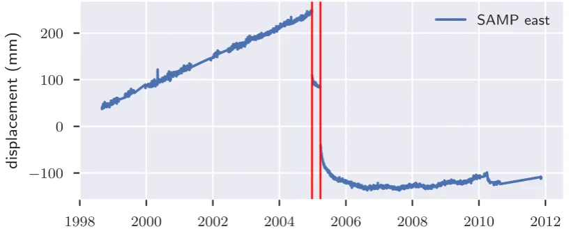
[image:34.595.63.473.187.358.2]

SAMP east

Figure 1.2: The east component of the position timeseries of the GPS station SAMP located at Sampali, Medan City, Indonesia. The red vertical lines mark the December 2004 Sumatra–Andaman earthquake as well as the March 2005 Nias-–Simeulue earthquake where coseismic discontinuities can be seen. Non-linear postseismic rebound signals are also visible here. The GLOBK [Herring et al.,2002] processed timeseries shown here is from Bock and Webb[2012, SOPAC archive].

The potential of the great earthquakes to cause measurable displacements of every geodetic station on Earth, including in particular the reference stations, poses a serious challenge to the integrity of the ITRF. It is not immediately obvious in this case how to calculate the coseismic offsets in the first place without the “fixed” far field [Kreemer et al., 2006]. Also, since the space geodetic technique with the best spatial resolution, GPS, is less sensitive to the CM than it is to the shape of its network, an overall movement of the whole network with respect to the CM is difficult to measure accurately with GPS. We will come back to this issue of GPS measurement of the geocentre motion momentarily in Section1.5. Nevertheless, due to the global nature of the disruption, the time-dependent reference coordinates in the ITRF would ideally have to be recalibrated after each great earthquake [Blewitt et al.,2010].

(35)

er-1.4. Impact of geophysical processes on the ITRF

rors that may reach up to∼0.2–0.4mm/yr. Furthermore, the sustained postseismic relaxation considerably far into the plates obfuscates plate boundaries, and contra-dicts the assumption of linearity of the velocity of the plates in the implementation of the NNR condition [Tregoning et al.,2013].

We are primarily interested in coseismic displacements in this thesis as an example process that we may model to be instantaneous. That is, we will ignore the viscoelastic properties of the mantle, and therefore its postseismic response, and concentrate solely on the Earth’s elasticity here.

Because of the global scale, the traditional dislocation theories in an elastic homogeneous half-space, such as Okada[1985], are not sufficient here. Instead, radially heterogeneous spherical Earth models, such asPollitz[1996], have proved to be valuable in modelling far field coseismic offsets. Failing to take into account the layered structure, along with the curvature, that is, the sphericity, of the Earth can introduce up to25% error in the static displacement calculated in the far field [Fu and Sun,2006;Banerjee et al.,2005].

There are, of course, other interesting effects that are not captured by the instantaneous surface displacement field. In general, earthquakes tend to deform the Earth towards a less oblate shape [Chao and Gross, 1987]. For instance, the Sumatra–Andaman earthquake is calculated to have reduced the oblateness of the Earth by ∼2×10−11_{, a subtle signal but nevertheless possibly measurable by} space geodesy. It is also estimated to have decreased the length of a day by ∼7 milliseconds (ms), and shifted the pole of rotation by ∼2milli-arc-seconds (mas) [Gross and Chao,2006].

1.4.2 Water movements and GRACE

(36)

2000 2002 2004 2006 2008 2010 2012 2014 2016

−50

−25

0 25 50

displacement

(mm)

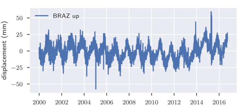
[image:36.595.65.471.129.314.2]

BRAZ up

Figure 1.3: The vertical component of the position timeseries of the GPS station BRAZ. The quasi-periodic signal here comes mostly from the Earth’s elastic response to the seasonal water mass movement in and out of the Amazon river basin. The GLOBK [Herring et al., 2002] processed timeseries shown here is fromBock and Webb[2012, SOPAC archive].

still need to be understood and systematically accounted for to ensure mm-level accuracy, precision and stability of the ITRF [see, for example, Collilieux et al.,

2010].

A truly enormous amount of surface water gets moved around seasonally. To support its massive weight, the Earth undergoes elastic deformation that is measur-able by satellite geodesy. For stations in regions of high hydrological activity such as river basins, or in areas with significant anthropogenic water mass movement, the displacements of the sites caused by the loading can be particularly significant. Fortunately, satellite gravimetry allows us to independently track movements of hydrological mass, in the forms of surface water, groundwater, ice or snow, by measuring the time-variable gravity field it creates. We can then deduce the con-tribution of the Earth’s elastic response to the weight of the redistributed water, assuming the rheology of the Earth is known, to the seasonal signals in the station position timeseries.

(37)

1.5. Geocentre motion

in 2002. It has been instrumental in studying and analysing long-term trends in the water cycle over the years because of its ability to detect mass variations of cm-level equivalent water heights. Its geospatial resolution,∼400km, is however somewhat coarse. Nevertheless, the elastic deformation corresponding to the mass movements observed by GRACE correlates well with GPS site position measurements [Tregoning et al.,2009;Zou et al.,2014].

Hence, in this thesis, we will adopt the time-variability of the mass distribution of the Earth, as seen by GRACE, as our model for surface water movement that serves as our illustrative case study of a continuous process deforming the Earth surface. Note, however, that in theory, the integrity of the RF suffers from neither the periodic component nor the linear trend in the station position timeseries, but is deteriorated only by non-linear trends that may result from, for instance, local water or oil extraction, or viscoelastic glacial isostatic adjustment (GIA).

1.5 Geocentre motion

The choice of the CM as the origin of our RF, as attractive as it is in theory, has a serious problem: being buried at the centre of the Earth, the CM is not physically accessible. We can “sense” the CM though via its gravitational influence. For example, it is possible to deduce its location from the orbits of the SLR satellites as they revolve around it.

Technologically advanced signal transmitters or receivers placed firmly on the Earth surface have been continually operating for decades. Naturally, space mea-surements of the positions of the ground stations, complemented by high-precision land survey at the co-location ties, can often be more accurate than the CM real-isation, although site-specific errors can also introduce large biases [Moore et al.,

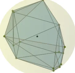
2014]. In fact, since GPS is a differential technique, it can determine the internal geometry of its network polyhedron even better [Bevis and Brown,2014]. Here, the internal geometry of the network is specified by the set of distances between the stations that are independent of the RF.

(38)

[image:38.595.207.329.146.263.2]

Figure 1.4: Schematic diagram of the network polyhedron of the geodetic stations (green dots) and the Centre of Mass (black star). The network polyhedron may be viewed as an approximation of the solid Earth surface (filled circle).

problem the other way around, and to try to locate and orient the CM frame with respect to the network. In this context, the CM is often referred to as the geocentre (GC), and hence, we are interested here in the precise determination of GC motion.

However, this network-dependent version of GC motion is theoretically rather inconvenient. In order to make contact with surface deformation models, for example, we need to characterise the GC motion in terms of the surface geometry alone, without references to specific networks. One such characterisation would be as the motion of the GC with respect to the entire surface of the solid Earth. The geodetic observation of the CM motion with respect to the network could then be viewed as the realisation of this theoretical construct, since the solid Earth surface is closely approximated by the surface of the network polyhedron.

But the surface of the Earth is not rigid, making it troublesome to interpret this characterisation in practice. We can circumvent this technical difficulty by introducing the Centre of Figure (CF) of the solid Earth surface [Trupin et al.,1992; Dong et al.,1997]:

rCF= 1 4π

Z

∂⊕

r0(θ,φ)dΩ (1.3)

(39)

1.5. Geocentre motion

from continuum mechanics. The Earth surface is here denoted by∂⊕, and dΩ= sinθdθdφ is the differential solid angle. The GC motion can be then defined as the motion of the CM with respect to the CF frame [see, for example, Wu et al.,

2012]. Note that the CF frame, in general, is not inertial.

GC motion is a key quantity of interest in geophysics in its own right because it signifies mass redistribution at the planetary scale. As such, careful measurements of GC motion can validate or constrain models of mass transport phenomena such as ocean and groundwater circulation, glaciation, or postseismic relaxation.

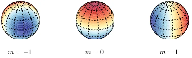
[image:39.595.171.481.304.398.2]

m=₋1 m= 0 m= 1

Figure 1.5: The three linearly independent modes of the (real, as opposed to complex) degree-1 spherical harmonics. Here, m denotes the order of spherical harmonics. The colours red and blue signify positive and negative values of the functions, respectively. Linear combinations of these three functions can express net transport across any plane that divides the sphere into equal halves.

Mathematically, GC motion is given by the degree-1components of the spherical harmonic decomposition of the surface displacement field. For surface water move-ments, the GC motion is the response to the corresponding degree-1 component of the surface water density that characterises a net transport of water from one hemisphere to the other (Figure 1.5), for instance. Part of the GC motion in this case results from the rigid translation of the solid Earth because of the recoil it experiences due to this net water transfer, and the rest may be attributed to the elastic deformation of the surface due to the loading of the redistributed water.

(40)

the special role of the degree-1spherical harmonics in the theory of GC motion in Section2.4.

Naturally, an error in the GC motion measurement translates to a hemisphere-scale correlated errors in the height of sea level [see, for instance, Beckley et al.,

2007; Melachroinos et al., 2013]. The impact of such an error on MSL becomes particularly significant if it happens to be roughly orthogonal to the nodal plane of the degree-1component of the ocean function3, that is, the plane that divides the Earth into two equal halves with the highest discrepancy in the oceanic areas.

Because of its special relationship with the inertial frame, the algorithm to calculate the degree-1components of the displacement field predicted by a crustal deformation model often differs from the one to calculate the higher degrees. Re-grettably, popular implementations often omit this exceptional case for simplicity [Xu and Chao,2015]. For example, ITRF2014, in a commendable attempt at incor-porating models of non-linear station motions into the ITRF, adopted the analytical formulae in Okada [1985] to model coseismic crustal deformation. But, being a half-space model, it not only fails to account for the sphericity of the Earth, it is completely unable to predict GC motion due to earthquakes.

Some space techniques (such as SLR) are more sensitive to the CM than others (such as VLBI). Accurate determination of the GC motion helps, alongside

co-location ties, to bind them together and to link them to satellite orbits. In particular, understanding GC motion is crucial for maintaining the stability of the RF over several decades. In addition, the precision of the GC measurement is a robust system performance indicator for space geodetic systems [Crétaux et al.,2002;Moore and Wang,2003;Kang et al.,2009].

Finally, we note that practical space geodetic measurement of GC motion has been difficult so far. Currently, it is hard to distinguish the SLR realisation of the GC motion from the background noise [Collilieux et al.,2009]. One of the principal hindrances here is the strong network effect of the relatively sparse SLR network. We, therefore, turn to the network effect next.

(41)

1.6. Network effect in geocentre motion measurements

1.6 Network effect in geocentre motion

measurements

We may view the GC motion, defined as the motion of the CM with respect to the figure of the solid Earth, as the physical quantity we want to measure. From this point of view, the motion of the CM with respect to the geodetic station network is a measurement, or a realisation, of the true GC motion. We will call the “error” in this measurement, that is, the discrepancy between the theoretical value of the GC motion and its practical measurement, the network effect (NE).

Just as we did in the last section, we get around the complications of defining motion with respect to a deforming network here by finding a point representative of the network called the Centre of Network (CN). As will be discussed further in Chapter3, it turns out that there are several distinct sensible definitions for CN. Perhaps the simplest one is the average of the positions of the stations [see, for example,Wu et al.,2012],

rCN= 1 N

N X

k=1

r0_k (1.4)

Here,N is the number of stations in the network, andr0_k is the position of thekth station on the deformed Earth. The theoretical GC motion is then the motion of CM with respect to the CF frame, or, the CM–CF motion, whereas its measurement by a geodetic network is the motion of the CM with respect to the CN frame, or, the CM–CN motion. The network effect, in this case, would be the CN–CF motion.

We should clarify that the CM–CN motion is of considerable value for RF reali-sation since it specifies how to position and orient the network in inertial space. In fact, it may appear that the true GC motion, that is, the CM–CF motion, is irrelevant to RF realisation, since the positions of the points other than the stations are not being measured anyway. However, the TRF is merely a realisation of the TRS that is self-consistently defined through geophysical modelling of the whole Earth, which inevitably involves consideration of the true GC motion.

(42)

of the term in Collilieux et al. [2010] seems to align more closely to the CM–CN motion itself.

The network effect, as defined here, arises because the geodetic network only samples the total displacement field of the crustal deformation processes at discrete, isolated points. If we could uniformly cover the entire Earth surface with geodetic stations then there would be no network effect. The NE therefore characterises the sampling bias that the finite network introduces. Intuitively, an evenly distributed set of sites that covers the whole Earth, although discrete, would reduce this bias, and therefore, the NE, if the network is sufficiently dense.

In practice, it is often not feasible to set up a dense network with an even coverage of the Earth surface. Most of the surface of the Earth is covered by oceans with practically inaccessible floors. Furthermore, the southern hemisphere has a greater share of oceanic area than the northern hemisphere. Even the continents do not have the same level of spatial coverage due to geographical and economical constraints. Also, reliable RF realisation requires well-understood trajectory models for its sites, so stations close to active volcanoes or tectonically deforming zones are not too helpful here.

Of course, the relatively sparser geodetic networks such as SLR and VLBI suffer more from the network effect. Unfortunately these two networks also happen to contribute the most to the realisation of the ITRF origin and scale. Thus the possibility of unmodelled or poorly modelled CM–CN motion aliasing into site coordinates remains a risk to the integrity and the stability of the ITRF [Wu et al.,

2011].

An exact determination of the NE in magnitude and direction, in principle, would allow us to measure the true GC motion within the current precision of space geodesy. Nevertheless, merely constraining the magnitude of NE effectively, as we propose to do in this thesis, helps us compare the predictions of deformation models with geodetic observations. When the models contain unknown parameters, the constraints on the magnitude of NE in turn restricts the domain of possible values for those parameters.

(43)

1.7. Thesis outline

these CNs are viewed as realisations of the same CF, the estimated magnitudes of the NE can serve as such a measure. Since network configurations change from time to time, we may also need to compare the temporal variation of CNs of the same network.

Lastly, despite our presentation of the NE here as an error, depending on the use case, NE of measurable size may not necessarily be detrimental to RF realisation. A case in point is coseismic deformation where a network of sites in the far field may remain virtually unaffected by the earthquake. The network in this case, in fact, facilitates the reconstruction of the RF, even though the calculated NE here is practically the same as the true GC motion.

1.7 Thesis outline

(44)

(45)

Chapter 2 Background

Here we introduce some of the ideas and results that our work builds upon. The goal is to establish terminology and notation, to set up the theoretical framework needed to model the geophysical processes of interest, and to present the mathematical consequences of the physical considerations that play key roles.

2.1 Helmert parameters of coordinate transform

Consider the relationship between the position vectorsr andr0_{of an arbitrary point} with respect to two different Cartesian coordinate systems. There are two basic transformations that preserve the Euclidean distances between points,

translation: r0=r+T (2.1a)

rotation: r0=Or (2.1b)

and thus can be used to transform r to r0. Here, T is an arbitrary vector and O represents an orthogonal matrix. Space geodetic techniques also consider an overall scale change,

scaling: r0= (1+D)r (2.2)

(46)

identity transform, the error associated with the choice of order is even smaller and hence can be neglected. In this case,O =1+A whereA is an infinitesimal anti-symmetric matrix. Thus,

r0=r+T+Dr+Ar=r+T+Dr+R×r (2.3)

whereRis the vector dual to the anti-symmetric matrixA. The parametersT, D, andRare the (instantaneous) Helmert parameters (HPs) of transformation between the two frames. Here,T, D,R, and the displacementu=r0−r experienced by the point under the transformation are all infinitesimals, or at least,

|T| |r|, |D| 1, |R| 1, |u| |r| (2.4) These conditions are well satisfied for the transformations between the reference frames of the different geodetic techniques, or the transformation between the undeformed and the deformed Centre of Figure (CF) frames that we consider next.

2.2 Shifts in Helmert parameters due to surface

deformation

For simplicity, we will consider here the effect of an arbitrary crustal deformation process in isolation. Our simplified model starts with an undeformed Earth that is spherically stratified, non-rotating, elastic, and isotropic, usually abbreviated as the SNREI Earth in the literature [Dahlen, 1968, see, for example]. Thus, the CF frame initially coincides with the Centre of Mass (CM) frame. The process under consideration then deforms the surface of the Earth, creating a displacement field u(r), and consequently, the CF frame moves (Figure 2.1). As in Section 1.5, we will adhere to the Lagrangian description in which the position vectorr refers to the position of the point on the undeformed Earth. Also, in the following, we will measure physical quantities, such as the displacementu here, with respect to the inertial CM frame unless indicated otherwise.

(47)

2.2. Shifts in Helmert parameters due to surface deformation

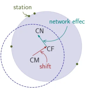
CM CF CN

network effect

[image:47.595.245.391.133.288.2]

shift station

Figure 2.1: Schematic diagram of the shift in the CF frame parameters of the deformed Earth (filled circle) with respect to the CM frame of the total undeformed Earth system (dotted circle), and the accompanying network effect, that is, the difference between the CN of geodetic stations (green dots) and the CF. The GC motion is the negative of the shifts in the CF frame parameters.

deformation of the Earth surface results in shifts in HPs of transformation from the CM frame to the CF frame. When several different processes are active on an already deformed Earth surface, as is the actual case, the observed changes in the CF frame parameters may be thought of as the sum of the shifts due to each of the processes.

In order to find expressions for the translational parameters T_CF, the scale parameter DCF, and the rotational parametersRCF, we consider the displacement fieldsv that the corresponding transformations would induce on the undeformed Earth surface. That is, as before, we consider the corresponding fields for the three groups of parameters,

v_T =TCF (2.5a)

vD=DCFr (2.5b)

v_R=RCF×r (2.5c)

(48)

R

∂⊕(u−v) 2

dΩin the transformed coordinates. The resulting expressions are,

TCF= 1 4π

Z

∂⊕

udΩ (2.6a)

D_CF= 1 4πr_⊕2

Z

∂⊕

r·udΩ (2.6b)

R_CF= 3 8πr_⊕2

Z

∂⊕

r×udΩ (2.6c)

where r_⊕ is the radius of the undeformed spherical Earth, ∂⊕denotes the Earth surface, anddΩ=sinθdθdφ is the differential solid angle. The first of these is essentially the definition of the CF [Trupin et al.,1992], the third appears inZhou et al.[2016] but, even though the derivation is straightforward, we have not come across the second in the literature yet.

For example, to derive the expressions for DCF, we set

∂ ∂DCF

Z

∂⊕

u−v_D2dΩ=0 (2.7)

or,

Z

∂⊕

u·rdΩ= Z

∂⊕

v_D·rdΩ=D_CF Z

∂⊕

r2dΩ=4πr_⊕2D_CF (2.8) The derivations for the other two are more involved and therefore we relegate them to AppendixB.2.

As we discussed in Section1.5, the geocentre (GC) motion is traditionally defined to be the motion of the CM with respect to the CF. We can justify this choice by noting that, although in inertial space it is really the surface of the Earth (along with the geodetic stations on it) that moves, from our point of view it is the CM that appears to move with respect to the network of geodetic stations. Therefore, the GC motion due to a surface deformation is the opposite of the CF frame motion that we considered here.

(49)

2.3. Vector spherical harmonics decomposition

2.3 Vector spherical harmonics decomposition

Any (square-integrable) vector field defined on and inside a sphere, such as the displacement fieldu in particular, can be expanded in terms of the vector spherical harmonics,

u = ∞ X

n=0 n X

m=−n

u_nm (2.9a)

u_nm=uS_nm+uT_nm (2.9b)

uS_nm(r,θ,φ) = y_1,S_nm(r)R_nm(θ,φ) +y_3,S_nm(r)S_nm(θ,φ) (2.9c) uT_nm(r,θ,φ) = y_1,T_nm(r)T_nm(θ,φ) (2.9d) The fieldu_nmis referred to as the mode with degreenand orderm. The components uS

nmandu T

nmare the spheroidal and toroidal parts of theunmmode respectively. The vector spherical harmonics themselves are

R_nm=Y_nmˆr (2.10a)

S_nm=∂Ynm ∂ θ θˆ+

1 sinθ

∂Y_nm

∂ φ φˆ =∇1Ynm (2.10b)

T_nm= 1 sinθ

∂Y_nm ∂ φ θˆ−

∂Y_nm

∂ θ φˆ =−ˆr× ∇1Ynm (2.10c) where the unit vectors(ˆr,θˆ,φˆ)correspond to the spherical coordinates(r,θ,φ) (de-fined in AppendixA.1),Y_nm(θ,φ)are the spherical harmonics (defined in Appendix

A.2),

∇1=θˆ ∂ ∂ θ +φˆ

1 sinθ

∂

∂ φ (2.11)

is the surface gradient operator on the surface of a sphere, and the normalisation and the orthogonality properties of the vector spherical harmonics are given in AppendixA.3. The radial functions y_1,S_nm, y_3,S_nm and y_1,nmT are the coefficients that characteriseuin this decomposition with respect to the basis consisting of the vector spherical harmonics in the space of (square-integrable) functions on the sphere. Since the displacement field u must be real, our conventions for the spherical harmonics imposes the relationships

(50)

for any of the y functions y₁T, y₁S, or y₃S, where superscript ∗ denotes complex conjugation. The symbolsR_nm andT_nm for the vector spherical harmonics are not to be confused with the symbolsRCFand TCF for the Helmert parameters.

There are significant advantages to this decomposition for our purposes. Per-haps most importantly, since our model of the Earth is spherically stratified, the equations of motion for the physical processes we will consider are decoupled in this representation. That is, the task of solving the equations for the total field reduces to solving simpler equations for each mode independently of the others. In fact, for the systems we consider, these equations can further be separated into spheroidal and toroidal parts. Moreover, the characteristic length-scale of the details captured by a particular mode is given by its associated wavelength

λn= 4πr⊕

2n+1 (2.13)

according to Jeans’ formula [see, for example, Tanimoto, 1986]. Hence we can truncate the infinite sum onnin Equation2.9at the level of details we desire to get an approximate field that is still continuous as a function. On a more practical note, since the indicesnand mare integers, the coefficients of this truncated expansion can be represented in the finite memory of a computer, possibly as an array.

2.4 Special role of degree-

0 and degree-

1 displacement fields

As far as transformations between the CM and the CF frames are concerned, the modes withn≤1are special. Evidently, the uniquen=0mode of the displacement field represents a uniform expansion or contraction, depending on the sign of the associated coefficient. Conversely, any overall scaling is represented only by the n= 0 mode since the other modes are orthogonal to it in the space of (square-integrable) vector fields on spheres. In other words, no mode with n 6= 0 can represent a global expansion or contraction.

(51)

2.4. Special role of degree-0and degree-1displacement fields

When we substitute the expansion in Equation 2.9 into Equation 2.6 for a displacement field u on the Earth surface r = r_⊕, we obtain explicit formulae of the CF parameters in terms of the coefficients of the vector spherical harmonic expansion,

T_CF= 1 4π

1 X

m=−1

y_1,1,mS (r_⊕) +2y_3,1,mS (r_⊕)∆_m (2.14a)

DCF= 1 p

4πr_⊕y S

1,00(r⊕) (2.14b)

R_CF= 3 8πr_⊕

1 X

m=−1

2y_1,1,mT (r_⊕)∆_m (2.14c)

where the constant vectors ∆_m are defined to be,

∆0=

v t4π

3 zˆ (2.15a)

∆1=−

v t2π

3 (ˆx+iˆy) (2.15b)

∆₋₁=−∆∗1=−

v t2π

3 (−ˆx+iˆy) (2.15c)

Here, the standard Cartesian unit vectors x,ˆ ˆy, and zˆ form a right-handed basis. Derivations of these formulae are presented in AppendixB.3. The exact expressions for ∆_m depends on the normalisation used for the spherical harmonics, but they can also be characterised by the normalisation-independent relation

ˆ r=

1 X

m=−1

Y_1,m∗ ∆_m (2.16)

as discussed in Appendix B.1. It is interesting to note that only the degree-1 spheroidal modes contribute to the translation parameters and, likewise, only the degree-1toroidal modes contribute to the rotation parameters, whereas only the degree-0mode contributes to the scale parameter.

(52)

rotation of the whole system under consideration must be able to be re-interpreted as a passive change of the coordinate system instead. In our case studies, this freedom shows up as degeneracies in the associated equations. Therefore we have to supplement the equations of motion with additional external information.

For the physical cases we consider, it turns out that the physical requirement of the conservation of linear and angular momenta are precisely the needed sup-plements [Okubo and Endo, 1986]. However, these laws only hold in an inertial reference frame, and the only obvious inertial frame available to us is the CM frame. Consequently, all our calculations are carried out in the CM frame. In this frame, the conservation laws take the form [Sun and Dong,2014],

Z

⊕

ρud V =0 (2.17a)

Z

⊕

ρr×ud V =0 (2.17b)

Here,⊕denotes the Earth interior,d V =r2d r dΩis the differential volume element, andρ(r)is the density of the layered Earth. As we derive in AppendixB.4, these conditions reduce to [Sun and Okubo,1993;Xu and Chao,2015],

Z r⊕

0

ρ y_{1, 1,m}S +2y_{3, 1,m}S r2d r =0 (2.18a) Z r_⊕

0

ρ y_{1, 1,m}T r3d r =0 (2.18b)

for|m| ≤1, respectively, for the vector spherical harmonics expansion of the dis-placement fieldu.

2.5 Theory of the elastic Earth

In Chapter4, we will study the coseismic GC motion caused by earthquakes and the associated network effect. In this section we present a sketch of the physical theory that enables us to calculate the coseismic displacement field.

(53)

2.5. Theory of the elastic Earth

simulate the Earth’s elastic response to such dislocations. To be more precise, we will consider the source to be composed of infinitesimal flat fault planes, each acting as a point source, whose effects are to be integrated in order to obtain the total coseismic field.

Also, we will model the coseismic displacement field to appear instantly at a fixed moment in time. Of course, neither is the earthquake actually instantaneous nor does its influence propagate instantly everywhere on the Earth. In the GPS station position timeseries data, the coseismic displacements are often seen to take place over several minutes. Roughly though, we expect the discontinuities, or offsets, in the daily GPS timeseries at the day of the earthquake to correspond to our modelled coseismic displacements. The relatively slower process of postseismic relaxation should preferably also be taken into account when calculating the offsets [Banerjee et al.,2005].

The dislocation theory of coseismic deformations was first developed for the half-space [Steketee, 1958; Press, 1965; Mansinha and Smylie, 1971; Okada,1985], but was soon adopted to take Earth’s sphericity into account [Ben-Menahem et al.,

1969;Smylie and Mansinha,1971;Wason and Singh,1972]. Despite their popularity, the half-space models are not adequate for our purpose of calculating the GC motion, since the infinite half-space is obviously infinitely massive. Our account of the theory here follows Pollitz[1992,1996] in part, since our implementation is adopted from his programSTATIC1D1. We augmented his code with the ability to calculate the degree-0and the degree-1modes crucial to the prediction of the CF frame parameters.

2.5.1 Equation of motion

Here we derive the displacement field for a point source following the Green’s function approach. The continuum version of Newton’s equation of motion, often called Cauchy’s equation, is

ρ∂ 2_u

∂t2 =f+∇ ·σ (2.19)

(54)

here, t denotes the time, ρ the density, σthe stress tensor, and f the body force density. The total moment tensorM for an arbitrary volumeV in this case may be expressed as [see, for example,Aki and Richards,2002, §3.4],

M = Z

V

f⊗r d V (2.20)

where⊗is the tensor product, that is, the dyadic product.

Static equilibrium is reached after the Earth responds elastically to the disloca-tion at the source, and hence the left hand side of Equadisloca-tion2.19 is zero here. In the absence of gravity, the body force density is also zero everywhere except at the point source located at r_s. Thus we re-write Equation 2.19 in the symbolic form [Pollitz,1996],

∇ ·σ=M· ∇δ r−r_s (2.21)

Here, M is the moment tensor at the source,∇is the vector differential operator, andδ is the Dirac delta. Fortunately, we will be able to incorporate the effect of the right hand side into the boundary conditions that we will consider later, rather than having to confront it directly. Hence for now, we consider the region where the right hand side of this equation is set to zero, that is, the whole Earth except the point source.

The most general linear constitutive relation between the stress and the strain for an elastic solid is often called the generalised Hooke’s law. In component form, it reads,

σi j=X

k,l

C_{i jkl}E_kl (2.22)

Here,C is a tensor of elastic moduli,

E =1

2 (∇u) + (∇u) T

(2.23)

is the strain tensor, and superscript T denotes the transpose. Since σ and E are symmetric, the most general form thatC can take for an isotropic material is [see, for example,Ben-Menahem and Singh,2012, §1.3],