Optimal Control for Multi-Mode Systems
with Discrete Costs
Mahmoud A. A. Mousa, Sven Schewe, and Dominik Wojtczak
University of Liverpool, Liverpool, U.K.
Abstract. This paper studies optimal time-bounded control in multi-mode sys-tems with discrete costs. Multi-mode syssys-tems are an important subclass of linear hybrid systems, in which there are no guards on transitions and all invariants are global. Each state has a continuous cost attached to it, which is linear in the sojourn time, while a discrete cost is attached to each transition taken. We show that an optimal control for this model can be computed in NEXPTIMEand approximated in PSPACE. We also show that the one-dimensional case is simpler: although the problem is NP-complete (and in LOGSPACEfor an infinite time horizon), we develop an FPTAS for finding an approximate solution.
1
Introduction
Multi-mode systems [8] are an important subclass of linear hybrid systems [4], which consist of multiple continuous variables and global invariants for the values that each variable is allowed to take during a run of the system. However, unlike for the full linear hybrid systems model, multi-mode systems have no guards on transitions and no local invariants. In this paper, we study multi-mode systems with discrete costs, which extend linear hybrid systems by adding both continuous and discrete costs to states. Every time a transition is taken (i.e. when the current state changes), the discrete cost assigned to the target state is incurred. The continuous cost is the sum of the products of the sojourn time in each state and the cost assigned to this state. Our aim is to minimise the total cost over a finite-time horizon or a long-time average cost over an infinite time horizon. We exemplify this by applying this model to the optimal control of heating, ventilation, and air-conditioning (HVAC) systems. HVAC systems account for about50%of the total energy cost in buildings [27], so a lot of energy can be saved by optimising their control. Many simulation programs have been developed to analyse the influence of control on the performance of HVAC system components such as TRNSYS [3], EnergyPlus [1], and the Matlab’s IBPT [2]. Our approach has the advantage over the existing control theory techniques that it provides approximation guarantees. Although the actual dynamics of a HVAC system is governed by linear differential equations, one can argue [24, 25, 22] that constant rate dynamic, as in our model, can approximate well such a behaviour.
on) as well as continuous costs.
When keeping an office building in a pleasant temperature range during opening hours, we face a control problem for multi-mode systems with a finite time horizon. We show that finding an optimal schedule in such a case is NP-complete and significantly more challenging than for the infinite time horizon (LogSPACE). However, we devise an FPTAS for the finite time horizon problem.
Heating multiple rooms simultaneously can be naturally modelled by multi-mode systems (with multiple dimensions). In such a scenario, we might have different pleasant temperature ranges in different rooms and the temperatures of the individual rooms may influence each other. Naturally, controlling a multi-dimensional multi-mode systems is more complex than controlling a one-dimensional multi-mode system. We develop a non-deterministic exponential time algorithm for the construction of optimal control, whose complexity is only driven by potentially required high precision in exponentially many mode switches. Allowing for anε-deviation from the ranges of pleasant temperatures reduces the complexity to PSPACE.
Related work. Our model can be viewed as a weighted extension of the linear hybrid automata model ([5, 17]), but with global constraints only. Even basic questions for the general linear hybrid automata model are undecidable already for three variables and not known to be decidable for two variables [9]. Most of the research for this model has focused on qualitative objectives such as reachability. Various subclasses of hybrid systems with a decidable reachability problem were considered, see e.g. [9] for an overview. In particular, reachability in linear hybrid systems, where the derivative of each variable in each state is constant, can be shown to be decidable for one continuous variable by using the techniques from [19]. In [6], it has been shown that reachability is decidable for timed automata, which are a particular subclass of hybrid automata where the slope of all variables is equal to 1.
In [22] we only studied the one-dimensional case of our model with the simplifying assumption that there is exactly one mode that can bring the temperature down and it is cost-free. In this paper, we drop this assumption and generalise the model to multiple dimensions. In the one-dimensional setting, we manage to prove similar nice algorithmic properties as in [22], i.e. the existence of finitely many patterns for optimal schedules, polynomial constant-factor approximation algorithm and an FPTAS. However, as opposed to the existence of a unique pattern for an optimal schedule in [22], we show that that there can be 44 different patterns when the simplifying assumption is dropped. To show this, we need to devise five safety-preserving and cost-non-increasing operations on schedules, while in [22] it sufficed for each mode to just lump together all timed actions that use this mode. Also, our constant-factor approximation algorithm requires a careful analysis of the interplay between different sections of the normal form for schedules, which results in anO(n7)algorithm, while in [22] it sufficed to use one mode
all the time and the algorithm ran in linear time.
horizon. Both of these papers show that, for any number of variables, a schedule with the optimal long-time average cost can be computed in polynomial time. In [24, 25], the same models without switching costs have been studied over the infinite time horizon, with the objective of minimising the peak cost, rather than the long-time average cost. In [11], long-time average and total cost games have been shown to be decidable for hybrid automata with strong resets, in which all variables are reset to0after each discrete transition. The long-time average and total cost optimisation for the weighted timed automata model have been shown to be PSPACE-complete (see e.g. [10] for an overview).
There are many practical approaches to the reduction of energy consumption and peak demand in buildings. One particularly popular one is model predictive control (MPC) [12]. In [26], stochastic MPC was used to minimise the energy consumption in a building. In [21], On-Off optimal control was considered for air conditioning and refrigeration. The drawback of using MPC is its high computational complexity and the fact that it cannot provide any worst-case guarantees. UPPAAL Stratego [15] supports the analysis of the expected cost in linear hybrid systems, but uses a stochastic semantics of these models [16, 14]. I.e. a control strategy induces a stochastic model where the time delay in each state is uniformly or exponentially distributed. This is different to the standard nondeterministic interpretation of the model, which we use in this paper. In [20], an on-line controller synthesis combined with machine learning and compositional synthesis techniques was applied for optimal control of a floor heating system.
Structure of the paper.The paper is organised as follows. We introduce all necessary notation and formally define the model in Section 2. In Section 3, we study the computa-tional complexity of limit-safe and-safe control in multiple dimensions. In Section 4, we show that in one dimension every schedule can be transformed without increasing its cost into a schedule following one of 44 different patterns. In Section 5, we show that the cost optimisation decision problem in one-dimension with infinite and finite horizon is LOGSPACEand NP-complete, respectively. In Section 6, still for the one-dimension case, we first show a constant factor approximation algorithm and, building on it, develop an FPTAS by a reduction to the 0-1 knapsack problem. Due to the space constraints, some of the proofs and algorithms are only available in the extended version of this paper [23].
2
Preliminaries
Let0N and1N beN-dimensional vectors with all entries equal to0and1, respectively. ByR≥0 andQ≥0 we denote the sets of all non-negative real and rational numbers,
respectively. We assume that0· ∞=∞ ·0 = 0. For a vectorv, letkvkbe its∞-norm (i.e. the maximum coordinate inv). We writev1≤v2if every coordinate vector of vector
v1is smaller than or equal to the corresponding coordinate in vectorv2, andv1< v2if, additionally,v16=v2holds.
2.1 Formal Definition of Multi-Mode Systems
tupleA= (M, N, A, πc, πd, Vmin, Vmax, V0)where:
– Mis a finite set of modes;
– N≥1is the number of continuous variables in the system; – A:M →QN is the slope of all the variables in a given mode;
– πc:M →Q≥0is the cost per time unit spent in a given mode;
– πd:M →Q≥0is the cost of switching to a given mode;
– Vmin, Vmax∈QN:Vmin< Vmax, define the safe set,S, as follows{x∈RN :Vmin≤
x≤Vmax};
– V0∈QN, such thatV0∈S, defines the initial value of all the variables.
2.2 Schedules, their cost and safety
Atimed actionis a pair (m, t) ∈ M ×R≥0 of a modemand time delayt > 0. A
scheduleσ(of lengthk) with time horizontmaxis a finite sequence of timed actions
σ=h(m1, t1),(m2, t2), . . . ,(mk, tk)i, such thatP k
i=1ti=tmax. Ascheduleσwith infinite time horizon is either an infinite sequence of timed actionsσ=h(m1, t1),(m2, t2), . . . ,(mk, tk), . . .i, such thatP
∞
i=1ti =∞or a finite sequence of timed actions
σ=h(m1, t1),(m2, t2), . . . ,(mk, tk)i, such thattk =∞. Therunof a finite schedule
σ=h(m1, t1),(m2, t2), . . . ,(mk, tk)iis a sequence ofstatesrun(σ) =hV0, V1, ..., Vkisuch that, for all0≤i≤k−1, we have thatVi+1=Vi+tiA(mi).
A schedule and its run are calledsafeifVmin≤Vi≤Vmaxholds for all1≤i≤k. A schedule and its run are called-safeifVmin−·1N < Vi < Vmax+·1N holds for all1≤i≤k. The run of an infinite schedule and its safety and-safety are defined accordingly.
Thetotal costof a scheduleσ=h(m1, t1),(m2, t2), . . . ,(mk, tk)iwith a finite time horizon is defined asπ(σ) =Pk
i=1πd(mi) +πc(mi)ti. Thelimit-average costfor a finite scheduleσ=h(m1, t1),(m2, t2), . . . ,(mk, tk)iwith an infinite time horizon is defined asπavg(σ) =πc(mk)and for an infinite scheduleσ=h(m1, t1),(m2, t2), . . .i it is defined as
πavg(σ) = lim sup k→∞
k
X
i=1
πd(mi) +πc(mi)ti
!
.Xk
i=1 ti
A safe finite scheduleσis-optimalif, for all safe finite schedulesσ0, we have that
π(σ0)≥π(σ)−. A safe finite schedule isoptimalif it is0-optimal. A safe infinite
scheduleσis optimalif, for all safe infinite schedulesσ0, we have thatπ
avg(σ0) ≥
πavg(σ).
The following example shows that there may not be an optimal schedule for a multi-mode system with a finite time horizon.
Example 1. Consider a multi-mode system with three modes:M1, M2, M3. The slope
vectors in these modes areA(M1) = (1,1),A(M2) = (1,−1)andA(M3) = (−1,1),
horizon betmax. Note that the following scheduleσ = (M1, ), (M2, t),(M3, t)
l
, wheret0 =tmax−,l=dt0/e, andt=t0/2l, has time horizontmaxand total cost >0. Ascan be made arbitrarily small but has to be>0,σis an-optimal schedule for all
>0, but no optimal schedule exists.
Note that in Example 1, for any >0, there exists an optimal-safe scheduleσwith total cost0:σ0 =h (M2, t),(M3, t)liwherelis defined as in Example 1. Our aim is to find an “abstract schedule” that, for any given >0, can be used to construct in polynomial time an-safe-optimal schedule.
LetM∗ ={m∈M |π
d(m) = 0}be the subset of modes without discrete costs. Note that, as shown in [8], the cost and safety of a schedule withM∗modes only, depends only on the total amount of time spent in each of theM∗modes. We therefore lump together any sequence of timed actions that only useM∗modes and define anabstract timed action (overM∗)as a functiont:M∗→R≥0. A finiteabstract schedulewith
time horizontmax(of lengthk) is a finite sequenceτ=ht1,(m1, t1),t2,(m2, t2), . . . , (mk−1, tk−1),tkisuch that∀imi∈M\M∗andPi≤k,m∈M∗ti(m)+Pi<kti=tmax.
The run of the abstract scheduleτis a sequencehV0, V1, . . . , V2k+1isuch that, for all i≤k, we haveV2i=V2i−1+A(mi)tiandV2i+1=V2i+Pm∈M∗A(m)ti(m). We say that an abstract schedule islimit-safeif its run is safe. The total cost of an abstract scheduleτis defined as
X
i≤k,m∈M∗
πc(m,ti(m)) +
X
i<k
πd(mi) +πc(mi)ti.
Note that any safe schedule can be turned into a limit-safe abstract schedule with the same cost by simply replacing any maximal subsequence of consecutive timed actions that only useM∗modes by a single abstract timed action. A limit-safe abstract schedule
σis optimal if the total cost of all other limit-safe abstract schedules is higher thanπ(σ). The following statement justifies the name “limit-safe”.
Proposition 1. Given a limit-safe abstract scheduleτand >0, we can construct in polynomial time an-safe scheduleσsuch thatπ(τ) =π(σ).
Proof. LetM∗ ={m1, m2, . . . , mj}. To obtainσfromτ, we replace each abstract timed action
m, tm)|m∈M∗ by a sequence (m1, tm1/l), . . . ,(mj, tmj/l) l
for a sufficiently largel∈N.
Sufficiently large means that, fort∗=P
m∈M∗tm,l > t∗·maxm∈M∗kA(m)k/. This choice guarantees thatP
m∈M∗kA(m)k ·tm/l < ε. Thus, when the abstract action
m, tm)|m∈M∗ joins two statesV2i, V2i+1along the runhV0, V1, . . . , . . . , V2k+1i
ofτ, we know that this concrete schedule will cover thel-th part ofV2i, V2i+1after every
sequence(m1, tm1/l),(m2, tm2/l), . . . ,(mj, tmj/l). As the safe set is convex, the start
and end points of this sequence are safe points. Also, P
m∈M∗kA(m)k ·tm/l < ε
implies that the points in the middle are-safe. ut
Example 1 continues.An example limit-safe abstract schedule of length 1 isτ =
{(m1, tmax/2),(m2, tmax/2)}. Based onτwe can construct an-safe scheduleh (m1, tmax/2l),(m2, tmax/2l)
l
2.3 Structure of optimal schedules
We show here that it later suffices to consider only schedules with a particular structure.
Definition 1. We call a finite scheduleσangularif there are no two consecutive timed actions(mi, ti),(mi+1, ti+1)inσsuch thatA(mi) =A(mi+1).
We show that while looking for an (-)safe (-)optimal finite schedule, we can restrict our attention to angular schedules only.
Proposition 2. For every finite (-)safe schedule with time horizontmaxthere exists an
angular safe schedule with the same or lower cost.
Henceforth, we assume that all finite schedules are angular. LetM0={m|A(m) = 0}, which we will also refer to aszero-modes.
Proposition 3. For every finite safe schedule with time horizontmaxthere exists a safe
schedule with the same or lower cost, in which at most one zero-mode is used at the very beginning.
Henceforth, we assume that all finite schedules use at most one zero-mode timed action and only at the very beginning.
2.4 Approximation algorithms
We study approximation algorithms for the total cost minimisation problem in multi-mode systems. We say that an algorithm is aconstant factor approximation algorithm
with arelative performanceρiff, for all inputsx, the cost of the solution that it computes,
f(x), satisfiesOP T(x)≤f(x)≤(1 +ρ)·OP T(x), whereOP T(x)is the optimal cost for the inputx. We are particularly interested in polynomial-time approximation algorithms. A polynomial-time approximation scheme (PTAS) is an algorithm that, for everyρ > 0, runs in polynomial-time and has relative performanceρ. Note that the running time of a PTAS may depend in an arbitrary way onρ. Therefore, we typically strive to find a fully polynomial-time approximation scheme (FPTAS), which is an algorithm that runs in polynomial-time in the size of the input and1/ρ.
The 0-1 Knapsack problem is a well-known NP-complete optimisations problem, which possess multiple FPTASes (see e.g. [18]). In this problem we are given a knapsack with a fixed volume and a list of items, each with an integer volume and value. The aim is to pick a subset of these items that together do not exceed the volume of the knapsack and have the maximum total value.
3
Complexity of limit-safe and
-safe finite control
As our one-dimensional model strictly generalises the simple linear hybrid automata considered in [22], we immediately obtain the following result.
Theorem 1 (follows from [22], Theorem 3). Given (one-dimensional) multi-mode systemA, constantstmaxandC(both in binary), checking whether there exists a safe
In the rest of this section we fix a (multi-dimensional) multi-mode systemAand time horizontmax.
Theorem 2. If a limit-safe abstract schedule exists inA, then there exists one of expo-nential length and it can be constructed in polynomial time.
Proof (sketch).Before we formally prove this theorem, we need to introduce first a bit of terminology. We call a modemsafe for timet >0atV ∈S:={x∈RN :Vmin≤
x≤Vmax}ifV +A(m)t∈S. Also,missafeatV if there existst >0such thatmis safe for timetatV. We say that acoordinate of a state,V ∈S,is at the borderif that coordinate inV is equal to the corresponding coordinate inVminorVmax.
Our algorithm first removes fromM all modes that will never be safe to use in a limit-safe schedule (and it can be found in the extended version of this paper [23]). This is an adaptation of [8, Theorem 7] where an algorithm was given for finding safe modes that can ever be used in a schedule with no time horizon. The main difference here is that the modes inM∗can always be used in a limit-safe abstract schedule even if they are not safe to use. We find here a sequence of sets of modesM∗=M0⊂M1⊂M2⊂. . .
suchMi+1is the set of modes that are safe at a state reachable fromV0via a limit-safe abstract schedule that only uses modes fromMi. Note that at some stepk≤ |M|this sequence will stabilise, i.e.Mk=Mk+1. Similarly as in the proof of [8, Theorem 7], we
can show that no mode fromM\Mkcan ever be used by a limit-safe abstract schedule. As a result, we can remove all these modes fromM.
Next, we remove all modes that cannot be part of a limit-safe abstract schedule with time horizontmax. For this, for eachm, we formulate a very similar linear programme (LP) as above (again, more details in [23]), where we ask for the time delay ofmto be positive and the total time delay of all the modes to betmax. By a simple adaptation of the proof of [8, Theorem 4], if this LP is not satisfiable thenmcan be removed fromA.
Next, we look for the easiest possible target stateVendthat can potentially be reached using a limit-safe abstract schedule fromV0with time horizontmax. For this,Vendhas to have the least number of coordinates at the border of the safe set. Note that this is well-defined, because ifV andV0 are two points reachable fromV0 via a limit-safe abstract schedulesτandτ0with time horizontmax, respectively, thenτ /2(i.e. divide all abstract and timed actions delays inτby 2) followed byτ0/2, is also a limit-safe abstract schedule with time horizontmax, which reaches(V +V0)/2. However,(V +V0)/2has a coordinate at the border iff bothV andV0have it as well. This shows that there is a state with a minimum number of coordinates at the border.
To find the coordinates that need to be at the border we will use the following LP. We have a variablexi for each dimensioni≤N and a constraint that requiresxito be less or equal to thei-th coordinate ofVmax−VendandVend−Vmin. We also add that
P
m∈Mtm=tmaxandVend =V0+Pm∈Mtm·A(m), with the objectiveMaximise
P
ixi. If the value of the objective is>0, we will get to know a new coordinate that does not have to be at the border. We then remove it from the LP and run it again. Once the objective is0, then all the remaining coordinates,I, have to be at the border and the solution to this LP tells us, at which border the solution has to be located (it cannot possibly be at the border of bothVminandVmaxas then we could reach the middle).
in the size of the input, we not only need a state with the minimum number of coordinates at the border, but also sufficiently far way from the border. Otherwise, we may need super-exponentially many timed actions to reach it. In order to find such a point, we replace allxi-s in the previously defined LP by a single variablexwhich is smaller or equal to all the coordinates ofVmax−VendandVend−VminfromI. We then set the objective toMaximisex, which will give us a suitable easy target stateVend.
Now, considerA0, which is the same asAbut with all slopes negated (i.e.A0(m) =
−A(m)for allm ∈ M). We claim thatVend is reachable fromV0using a limit-safe abstract scheduleτiff(V0+Vend)/2is reachable fromV0inAwith time horizontmax/2 and(V0+Vend)/2is reachable fromVend inA0 with time horizontmax/2; this again follows by consideringτ /2. Note that a coordinate of(V0+Vend)/2is at the border iff it is at the border in bothV0andVend.
This way we reduced our problem to just checking whether a limit-safe abstract schedule exists from one point to another more permissive point (i.e. where the set of safe modes is at least as big) within a given time horizon. The algorithm that solves this problem is provided in the extended version. It again reuses the same constructions as above, e.g. by constructing a sequence of sets of modesM∗=M0⊂M1⊂. . .⊂Mk, and its correctness follows similarly as before. We now need to invoke this algorithm twice: to check that(V0+Vend)/2is reachable fromV0with time horizontmax/2and that(V0+Vend)/2is reachable fromVendwith time horizontmax/2inA0. If at least one of these calls return NO, then no limit-safe abstract schedule fromV0toVendcan exist. Otherwise, letσandσ0be the schedules returned by these two calls, respectively. Then the concatenation ofσwith the reverse ofσ0is a limit-safe abstract schedule that reaches
VendfromV0with time horizontmax. ut
Theorem 3. Finding an optimal limit-safe abstract schedule inAcan be done in non-deterministic exponential time.
Proof. The limit-safe abstract schedule constructed in Theorem 2 has an exponential length. To establish a nondeterministic exponential upper bound, we can guess the modes (and the order in which they occur). With them, we can produce an exponentially sized linear program, which encodes that the run of the abstract schedule is safe and minimises
the total cost incurred. ut
Theorem 3 and Proposition 1 immediately give us the following.
Corollary 1. If a limit-safe abstract schedule exists inA, then for any >0an-safe schedule with the same cost can be found in nondeterministic exponential time.
Moreover, from Theorem 2 and the fact that in the case of multi-mode systems with no discrete costs all abstract schedules have length1, we get the following.
Corollary 2. Finding an optimal limit-safe abstract schedule for multi-mode systems with no discrete costs can be done in polynomial time.
Theorem 4. If a limit-safe abstract schedule exists, then finding an-safe-optimal strategy can be done in deterministic polynomial space.
Proof. When reconsidering the linear programme from the end of the proof of Theorem 3, we can guess the intermediate states in polynomial space (and thus guess and output the schedule) as long as all states along the run (including the time passed so far) are representable in polynomial space.
Otherwise we use the opportunity to deviate by up tofrom the safe set by increasing or decreasing the duration of each timed action up to someδ > 0, in order to keep the intermediate values representable in space polynomial in|A|and. However, we apply these changes in a way that the overall time remainstmax. Clearly this is possible, because withinδ/2of the actual time point of each state along the run, there is a value whose number of digits in the standard decimal notation is at most equal to the sum of the number of digits inδ/2andtmax. Picking any such point for every interval would induce a schedule with the required property and they can be simply guessed one by one. The final imprecision introduced by this operation is at mostb·δ·maxm∈M|A(m)|, wherebis a bound on the number of timed actions in a limit-safe schedule, which is exponential in|A|. If we chooseδ =/(b·maxm∈M|A(m)|), then we will get the required precision.
Although our algorithm is nondeterministic, due to Savitch’s theorem, it can be
implemented in deterministic polynomial space. ut
4
Structure of Finite Control in One-dimension
We show in this section that any finite safe schedule in one-dimension can be transformed without increasing its cost into a safe schedule, which follows one of finitely many regular patterns. The crucial component of this normal form will be a “leap” that we define below. We first introduce some notation. LetM+ = {m | A(m) > 0} and
M− ={m|A(m)<0}. Recall thatM0={m|A(m) = 0}. We will call a mode,m, anup mode, down mode, or zero-modeifm∈M+,m∈M−, orm∈M0, respectively. Similarly, thetrendof a timed action(m, t)isup, down, flatifmis an up, down, zero-mode, respectively. For any subsequence of timed actionsσ0 =h(m
i, ti), . . . , (mj,
tj)iin a scheduleσ, whose run isrun(σ) =hV0, V1, . . . , Vki, we say thatσ0starts at
statevandends at statev0iffv=Vi−1andv0 =Vj. We use the same terminology for a single timed action (in this case this subsequence has length 1).
Definition 2. Apartial leapis a pair of consecutive timed actions(mi, ti),(mi+1, ti+1)
in a safe schedule such thatmi∈M+,mi+1∈M−, andA(mi)ti+A(mi+1)ti+1= 0,
i.e. the state of a multi-mode system does not change after any partial leap. A partial leap iscompleteifA(mi)ti =Vmax−Vmin. We will simply refer to complete leaps as leaps.
There are|M+×M−|types of leaps. A leap is oftype(m, m0)∈M+×M−iff mi =mandmi+1 =m0. Let∆tmand∆πmdenote the time and cost it takes for an
up modemto get fromVmintoVmaxor a down modemto get fromVmaxtoVmin. Note
that∆tm=|(Vmax−Vmin)/A(m)|and∆πm=πd(m) +πc(m)·∆tm. By∆tm,m0and ∆πm,m0we denote the time duration and the cost of a leap of type(m, m0)∈M+×M−,
Any safe scheduleσcan be decomposed into three sections that we will call itshead, leaps, and tail. Thehead sectionends after the first timed action that ends atVmin. The
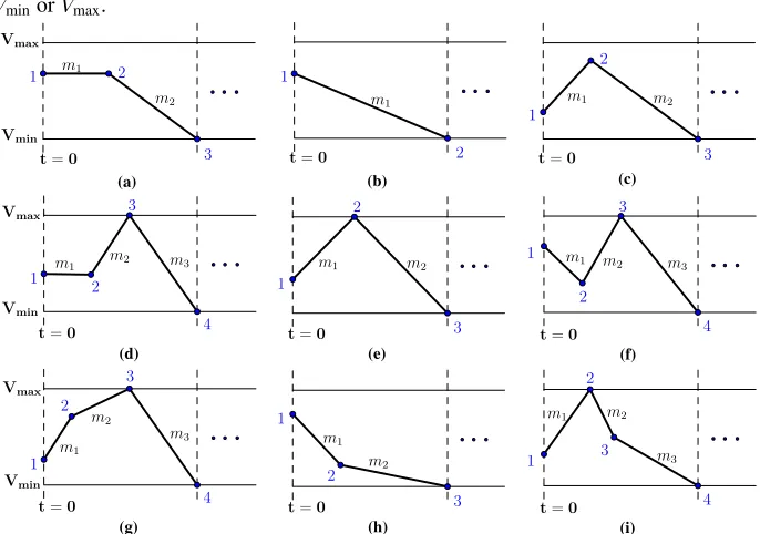
leaps sectioncontains only leaps of possibly different types following the head section. Finally, thetail sectionstarts after the last leap in the leaps section has finished. Note that any of these sections can be empty and the tail section can in principle contain further leaps. We show here that, for any safe schedule of length at least three, there exists another safe one with the same or a smaller cost, whose head and tail sections follow one of the 10 patterns presented in Figure 3 and Figure 4, respectively, where
partial up/downmeans that the next state is not at the border. For each of these patterns, there exists an example which shows that an optimal safe schedule may need to use such a pattern and hence it is necessary to consider it. In order to prove this, we first need to define several cost-nonincreasing and safety-preserving operations that can be applied to safe schedules. These will later be applied in Theorem 5 to transform any safe schedule into one of the just mentioned regular patterns. These operations are easy to explain via a picture, but cumbersome to define formally. Therefore, the formal definitions can be found in the extended version of this paper [23] and we present here only the intuition behind them.
Letσbe any safe finite schedule. Following Proposition 2 and 3, we can assume thatσis angular and only contains at most one timed action with a zero-mode, and if it contains one, this action occurs at the very beginning. Unless explicitly stated, the operations below are defined for timed actions with up or down trend only.
Vmax
Vmin
1 2
m1 3 m2
4 m3
20
m2
30 m3
m1
Vmax
Vmin
1 2
m1
3 m2
4
m3
5 m4 20
m3
30
m4 40
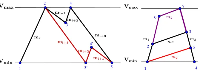
[image:10.612.142.479.376.457.2]m1m2
Fig. 1: On the left, the rearrange operation applied to three timed actions 1-2-3 with modesm1, m2, m3results in 1’-2’-3’ with modesm2, m3, m1. On the right, the shift
operation is being applied to a partial leap 1-2-3 which will be moved after the (complete) leap 3-4-5.
The first operation that we need is therearrangeoperation, which simply changes the order of any subsequence of timed actions with the same trend. The next one is the
shiftoperation. It cuts any subsequence of timed actions that start and end at the same state,V, and pastes this subsequence after any timed action that ends atV. The effect of these two operations can be seen in Figure 1.
Vmin Vmax
1
2
mi
3 mi+1
4
mi+2
5 mi+3
3’
mi+3 4’
mi+2
mi+1 V
min
Vmax
1 2
m1
3
m2
4
m3
7
6 m2
5
[image:11.612.141.476.115.233.2]m2
Fig. 2: On the left, an example of applying the shift-down operation to timed actions
mi+1, mi+2. These actions are rearranged to move after point 5, which becomes point
3’ (i.e. following timed actionmi+3). On the right, an example of applying the wedge
operation to three timed actionsm1, m2, m3. This operation is a (parallel) translation
of the actionm2, which changes the time duration of each of theses actions. After this
operation either them2line touchesVmin, which would removem1from the schedule,
or them2line touchesVmax, which would change a state along the run of the schedule to be at the border.
or down, until either the timed actionm1is removed orm2ends atVmax. The direction depends on the cost gradient, but as the cost delta function of this operation is linear, one of these directions is cost-nonincreasing.
Finally, we define theresizeoperation that will be used the most in our procedure. The resize operation requires one parametert∈Rand can act on any two consecutive timed actions in a safe schedule. Intuitively, ift <0, this operation decreases the total time of this pair of timed actions by|t|while changing only the middle state between these two timed actions along the run of the schedule. Ift >0, this operation increases the duration of this pair of timed actions by t while again changing only the state between them along the run. Ift >0then we will also refer to this operation as the
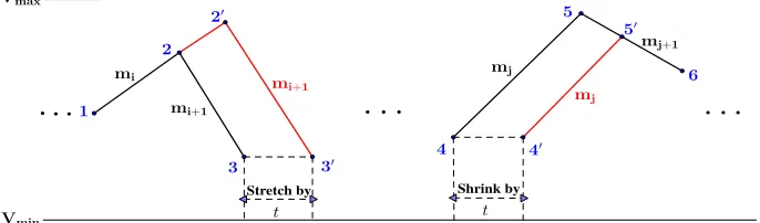
stretchoperation and ift <0as theshrinkoperation with parameter−t >0. If the stretch and shrink operations are simultaneously applied with the same parametertto two non-overlapping pairs of timed actions, the result is a safe schedule with the same time horizon as before, but with a possibly different total cost. We will call aflexiany subsequence of length2in a safe schedule such that both shrink and stretch operations can be applied to it for somet >0without compromising its safety. A simultaneous application of these two operations to flexis is demonstrated in Figure 5 and 6.
Consider two non-overlapping flexis at positionsiandjin a safe scheduleσ. Let
σ0 = resize(σ, i, t)be the resulting schedule of applying the resize operation with
parameter tto the i-th and i+ 1-th timed actions inσ andresize-domain(σ, i)be the maximal closed interval from which t can be picked to ensure that σ0 is safe. Similarly, letσ00 = resize(σ, j,−t)andσ000 = resize(resize(σ, i, t), j,−t)). Note that
σ000has the same time horizon asσand it is safe as long ast∈resize-domain(σ, i)∩
resize-domain(σ, j)and let us denote this closed interval byI. Furthermore,π(σ000)−
intin the interior ofI. As a result,π(σ000)−π(σ)is also a linear function intand so its minimum value is achieved at one of the endpoints ofI. Also, at such an endpoint, one of the time actions in these two flexis will disappear and as a result the total cost would be reduced even further. It follows, that there is an endpoint ofIsuch that selecting it astwill not increase the cost of the schedule, but it will remove a flexi fromσ. As the zero-mode timed action and the last timed action in a schedule can have flexible time delay, we can also define the resize operation for them in a similar way. As a result, we can apply the resize operation with parametertto any of these (including a flexi) and with parameter−tto the other. Reasoning as above, there is a value fortsuch that the cost of the resulting schedule does not increase, the schedule remains safe, and at least one of the timed actions is removed fromσor one more state along the run ofσbecomes
VminorVmax.
t=0 t=0 t=0
t=0 t=0 t=0
Vmax
Vmax Vmin
Vmin
(a) (b) (c)
(d) (e) (f)
t=0 t=0 t=0
(g) (h) (i)
Vmax
Vmin
1 m1 2
[image:12.612.138.481.252.493.2]3 m2 1 2 m1 1 2 m1 3 m2 1 2 m1 3 m2 4 m3 1 2 m1 3 m2 1 2 m1 3 m2 4 m3 1 2 m1 3 m2 4 m3 1 3 1 2 m1 4 2 m1 m2 3 m2 m3
Fig. 3: Ten possible head patterns: (a) flat+down (b) down (c) partial-up+down (d) flat+up+down (e) up+down (f) partial-down+up+down (g) partial-up+up+down (h) partial-down+down (i) up+partial-down+down and (j) empty (not depicted).
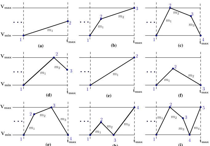
Theorem 5. For every safe scheduleσin a one-dimensional multi-mode system there exists a safe scheduleσ0whose head section matches one of the patterns in Figure 3, tail section matches one of the patterns in Figure 4, andπ(σ0)≤π(σ)holds. Furthermore, it suffices to consider only 44 combinations of these head and tail patterns, and the length of all of them is at most five.
Proof. We will repeatedly apply combination of shrink and stretch operations to flexis until we remove all non-overlapping ones. Note that after each such an application either a timed action is removed or one more state along the run ofσbecomes equal toVmaxor
Vmax Vmin tmax Vmax Vmin (a) tmax (d) tmax (e)
tmax tmax
(g) (h)
tmax tmax
(b) (c) tmax (f) (i) Vmax Vmin tmax 1 2 m1 1 2
m1 3
m2 1 2 m1 4 3 m3
2 m2
1 m1 1 2 m1 3 m2 4 m3 4 1 2 m1 3 m2 1 2 m1 3 m2 m3 1 2 m1 3 m2 5 1 2
m1 m2 3
[image:13.612.138.479.112.350.2]4 m3 m4
Fig. 4: Ten possible tail patterns: (a) partial-up (b) partial-up+up (c) up+partial-down+down (d) up+partial-down (e) up (f) partial-up+down (g) partial-up+up+down (h) partial-up+down+up (i) up+partial-down+down+up and (j) empty (not depicted).
1. as long as there are at least one pair of non-overlapping flexis then shrink one and stretch the other until a timed action is removed or a new state at the border is created;
2. once there is only one flexi left or two overlapping ones, use the shift or shift-down operation to move them to the end of the schedule;
3. if the first timed action is flat, pair it with the remaining flexi to remove one of them using the shrink-stretch operation combination;
4. if the last state ofrun(σ)is not at the border and a flexi or flat timed action remains after the previous step, they should be paired with each other for the shrink-stretch operation combination;
5. if two overlapping flexis exist, use the wedge operation to resolve them;
6. finally, if the tail section still does not follow any of the patterns, apply the shift-down operation to the (unique) segment that starts and ends atVmax.
using one of these operations, results in Figure 3 for the head section and Figure 4 for the tail section.
If we try to combine all these head and tail pattern together then this would result in 10·10 = 100possible combinations. However, as just mentioned, there can be only one point not at the border or a zero-mode timed action in a schedule so these combinations of head and tail patterns can be reduced further. In particular, any head pattern can be combined with tail patterns (e) and (j), but only (b), (e), (j) head patterns can be combined with the remaining tail ones. Therefore, there are10·2 + 3·8 = 44combined patterns and it is easy to check that none of them has length larger than five (this is important for the computational complexity stated in Theorem 8). ut
Vmin Vmax
Stretch by Shrink by
1 2
m1
3
m2
10
20
m3
30
m4 5
4
m2
t
40
50
m3
[image:14.612.138.483.247.349.2]t
Fig. 5: Shrink and stretch operations being applied to two up-up flexis. The 1-2-3 one is stretched byt, which results in 1-4-5, and 1’-2’-3’ is shrunk byt, which results in 4’-5’-3’. Note that 3 and 5 (also, 1’ and 4’) are the same states but shifted in time. In fact, all states along the run of the schedule stay the same apart from 2 and 2’, and as a result the schedule stays safe.
Stretch by Shrink by
Vmin Vmax
1
2
mi
3 mi+1
4
5
mj 6
mj+1
20
30 mi+1
40
50
mj
t t
Fig. 6: Shrink and stretch operations being applied to two up-down flexis.
5
Complexity of Optimal Control in One-dimension
We start with considering the easy case of infinite time horizons, before turning to the interesting case of finite time horizons.
5.1 Infinite time horizon
First let us consider the caseM0=∅. If alsoM+×M−=∅then there are no safe
[image:14.612.138.481.432.533.2]Let us pick any modem−∈M−and denotet−:= (Vmin−V0)/A(m−). Consider the infinite scheduleσ, which starts with the timed action(m−, t−)followed by infinitely many complete leaps of type(i0, j0). Obviously, at all timest=t−+k·∆ti0,j0where k∈N,σis more expensive by at mostπd(m−) +πc(m−)t−from the cheapest schedule with time horizont. Consequently, ask→ ∞, this shows that the limit superior of the average cost cannot be smaller than∆πi0,j0/∆ti0,j0. At the same time,σrealises this long-time average.
IfM0 6= ∅, then let m0 = min
m∈M0πc(m)be the zero-mode with the lowest continuous cost to run. We claim that ifπc(m0)< ∆πi0,j0/∆ti0,j0 orM+×M−=∅ then an optimal safe schedule is simply(m0,∞), whose limit-average cost isπc(m0), and otherwiseσdefined above is an optimal safe schedule. This is because, ifπc(m0)<
∆πi0,j0/∆ti0,j0, then, at any time point ofσwhere a leap of some type(i, j)is used, removing this leap and increasing the timem0is used for by∆ti,jreduces the total cost up to this time point.
Taking into account thatargmin(i,j)∈M+×M−∆πi,j/∆ti,jcan be computed using logarithmic space (because multiplication, division and comparison can be [13]) we get the following theorem.
Theorem 6. An optimal safe infinite schedule for one-dimensional multi-mode systems can be computed in deterministicLOGSPACE.
5.2 Finite Time Horizon
Due to Theorem 1, we already know that the decision problem for optimal schedules in one-dimensional multi-mode systems is at least NP-hard. Here, we show that the problem is NP-complete by showing that an optimal schedule exists and that each section of an optimal schedule can be guessed.
Note that the existence of an optimal schedule for the one-dimensional case sets it apart from the general case. In Example 1, we have shown that optimal schedules are not even guaranteed to exist for two-dimensional multi-mode systems.
Theorem 7. For any one-dimensional multi-mode systemsAandtmax≥0, there exists
an optimal schedule with time horizontmax, and checking for the existence of an optimal
schedule with cost≤CisNP-complete. (WhentmaxandCare given in binary.)
Proof. First, we can simply iterate over all schedules of length one and directly calculate their costs. Next, we can iterate over pairs of modes,m1andm2, and for each of them solve a linear program (LP) which will give us the cheapest schedule of length two using these two modes. This LP finds the cheapest partition oftmaxbetween the two modes and has the following form: Minimiseπc(m1)t1+πc(m2)(tmax−t1) +πd(m1) +πd(m2)
Subject to:0≤t1≤tmax, Vmin≤V0+A(m1)t1≤Vmax and
Vmin≤V0+A(m1)t1+A(m2)(tmax−t1)≤Vmax. This can be done inO(|A|2)time.
may be empty). Due to Theorem 5, there are 44 combined patterns for the tail and head sections. Note that, when considering only the cost of the whole schedule, it suffices for us to know the number of leaps of each type in the leaps section and not their precise order. Notice that a schedule with time horizontmaxcan contain at mostbtmax/∆πi,jc leaps of type(i, j). The size of this number is polynomial in the size of the inputA. There areO(|M|2)types of leaps so the number of leaps of each type and the combined
pattern of the schedule can be guessed non-deterministically with polynomially many bits. This guess uniquely determines the cost of the schedule. This is because, after the total time of the leaps section is deducted fromtmax, we get the exact time the head and tail section have to last for. Each combined pattern has at most one of the following: a flexi, a zero-mode, or the last state not at the border. The time remaining will determinate exactly (if at all possible) the value of this single flexible point along this schedule. Now, computing the cost of the resulting schedule and checking whether it is lower thanC
can be done in polynomial time. This shows that the problem is in NP. It also shows that optimal schedules exist, because there are only finitely many options to choose from. ut
6
Approximate Optimal Control in One-Dimension
We first show an approximation algorithm with a3-relative performance for the cost minimisation problem in one-dimensional multi-mode systems, which runs inO(|A|7)
time. Our algorithm tries all possible patterns for an optimal schedule and for the leaps section always picks leaps of the same type. It then adds, if necessary or for cost efficiency, a partial leap to the leaps section and minimises the total cost of the just constructed schedule by optimising the time duration of this partial leap. This constant approximation algorithm is crucial for showing the existence of an FPTAS for the same problem in the next subsection.
Theorem 8. Computing a safe schedule with total cost at most three times larger than the optimal one for one-dimensional multi-mode systemAcan be done inO(|A|7)time.
We now show that the cost minimisation problem for one dimensional multi-mode systems is in FPTAS by a polynomial time reduction to the 0-1 Knapsack problem, for which many FPTAS algorithms are available (see e.g. [18]). This is similar to the FPTAS construction in [22], but differs in how the modes with fractional duration are handled. First we iterate over all possible schedules of length at most two and find the cheapest one in polynomial time. Next, thanks to Theorem 5, all optimal schedules longer than two can be transformed into one of 44 different patterns. Each of these patterns results in a slightly different FPTAS formulation. An FPTAS for the general model consists of all of these individual FPTASes executed one after another. The details of the proof are provided in the extended version.
Theorem 9. Solving the optimal control problem for multi-mode systems with relative performanceρtakes O(poly(1/ρ)poly(size of the instance))time and is therefore in FPTAS.
Acknowledgement
References
1. EnergyPlus: Building energy simulation program.https://energyplus.net/. 2. IBPT: International Building Physics Toolbox in Simulink.http://www.ibpt.org/. 3. TRaNsient SYstems Simulation Program.http://sel.me.wisc.edu/trnsys/. 4. Rajeev Alur, Costas Courcoubetis, Nicolas Halbwachs, Thomas A. Henzinger, P.-H. Ho,
Xavier Nicollin, Alfredo Olivero, Joseph Sifakis, and Sergio Yovine. The algorithmic analysis of hybrid systems.Theoretical computer science, 138(1):3–34, 1995.
5. Rajeev Alur, Costas Courcoubetis, Thomas Henzinger, and Pei Ho. Hybrid automata: An algorithmic approach to the specification and verification of hybrid systems. InHybrid Systems, pages 209–229. Springer Berlin / Heidelberg, 1993.
6. Rajeev Alur and David L. Dill. A theory of timed automata.Theoretical Computer Science, 126(2):183–235, April 1994.
7. Rajeev Alur, Vojtech Forejt, Salar Moarref, and Ashutosh Trivedi. Safe schedulability of bounded-rate multi-mode systems. InHSCC, pages 243–252. ACM, 2013.
8. Rajeev Alur, Ashutosh Trivedi, and Dominik Wojtczak. Optimal Scheduling for Constant-Rate Multi-Mode Systems. InProc. of Hybrid Systems: Computation and Control 2012. 9. Eugene Asarin, Venkatesh P. Mysore, Amir Pnueli, and Gerardo Schneider. Low dimensional
hybrid systems – decidable, undecidable, don’t know.Information and Computation, 211:138– 159, February 2012.
10. Patricia Bouyer. Weighted Timed Automata: Model-Checking and Games.Electronic Notes in Theoretical Computer Science, 158:3–17, May 2006.
11. Patricia Bouyer, Thomas Brihaye, Marcin Jurdzi´nski, Ranko Lazi´c, and Michał Rutkowski. Average-Price and Reachability-Price Games on Hybrid Automata with Strong Resets. In Franck Cassez and Claude Jard, editors,Formal Modeling and Analysis of Timed Systems, number 5215 in Lecture Notes in Computer Science, pages 63–77. Springer Berlin Heidelberg, September 2008.
12. Eduardo F Camacho and Carlos Bordons Alba.Model predictive control. Springer Science & Business Media, 2013.
13. Andrew Chiu, George I. Davida, and Bruce E. Litow. Division in logspace-uniformNC1. ITA, 35(3):259–275, 2001.
14. Alexandre David, Dehui Du, Kim Guldstrand Larsen, Axel Legay, and Marius Mikuˇcionis. Optimizing Control Strategy Using Statistical Model Checking. In Guillaume Brat, Neha Rungta, and Arnaud Venet, editors,NASA Formal Methods, number 7871 in Lecture Notes in Computer Science, pages 352–367. Springer Berlin Heidelberg, May 2013.
15. Alexandre David, Peter Gjøl Jensen, Kim Guldstrand Larsen, Marius Mikuˇcionis, and Jakob Haahr Taankvist. Uppaal Stratego. In Christel Baier and Cesare Tinelli, editors,
Tools and Algorithms for the Construction and Analysis of Systems, number 9035 in Lecture Notes in Computer Science, pages 206–211. Springer Berlin Heidelberg, April 2015. 16. Alexandre David, Kim G. Larsen, Axel Legay, Marius Mikuˇcionis, and Zheng Wang. Time
for Statistical Model Checking of Real-Time Systems. In Ganesh Gopalakrishnan and Shaz Qadeer, editors,Computer Aided Verification, number 6806 in Lecture Notes in Computer Science, pages 349–355. Springer Berlin Heidelberg, July 2011.
17. Thomas A. Henzinger. The theory of hybrid automata. InProc. of the 11th IEEE LICS’96 Symposium, Washington, DC, USA, 1996.
18. Hans Kellerer, Ulrich Pferschy, and David Pisinger. Knapsack Problems. Springer Berlin Heidelberg, Berlin, Heidelberg, 2004.
20. Kim G Larsen, Marius Mikuˇcionis, Marco Muniz, Jiˇr´ı Srba, and Jakob Haahr Taankvist. Online and compositional learning of controllers with application to floor heating. In Inter-national Conference on Tools and Algorithms for the Construction and Analysis of Systems, pages 244–259. Springer, 2016.
21. Bin Li and Andrew G. Alleyne. Optimal on-off control of an air conditioning and refrigeration system. InAmerican Control Conference (ACC), 2010, pages 5892–5897. IEEE, 2010. 22. Mahmoud A. A. Mousa, Sven Schewe, and Dominik Wojtczak. Optimal control for simple
linear hybrid systems. In23rd International Symposium on Temporal Representation and Reasoning (TIME), pages 12–20. IEEE, 2016.
23. Mahmoud A. A. Mousa, Sven Schewe, and Dominik Wojtczak. Optimal Control for Multi-Mode Systems with Discrete Costs.CoRR, ???????????????????, 2017.
24. Truong X. Nghiem, Madhur Behl, Rahul Mangharam, and George J. Pappas. Green scheduling of control systems for peak demand reduction. InDecision and Control and European Control Conference (CDC-ECC), 2011 50th IEEE Conference on, pages 5131–5136. IEEE, 2011. 25. Truong X. Nghiem, George J. Pappas, and Rahul Mangharam. Event-based green scheduling
of radiant systems in buildings. InAmerican Control Conference (ACC), 2013, pages 455–460. IEEE, 2013.
26. Frauke Oldewurtel, Andreas Ulbig, Alessandra Parisio, G¨oran Andersson, and Manfred Morari. Reducing peak electricity demand in building climate control using real-time pricing and model predictive control. InDecision and Control (CDC), 2010 49th IEEE Conference on, pages 1927–1932. IEEE, 2010.
27. Luis P´erez-Lombard, Jos´e Ortiz, and Christine Pout. A review on buildings energy consump-tion informaconsump-tion.Energy and buildings, 40(3):394–398, 2008.