DEVELOPMENT OF ADVANCED RADIATION
MONITORS FOR PULSED NEUTRON FIELDS
Thesis submitted in accordance with the requirements of the
University of Liverpool for the degree of Doctor in Philosophy
by
Giacomo Paolo Manessi
1
Abstract
The need of radiation detectors capable of efficiently measuring in pulsed neutron fields is attracting
widespread interest since the 60s. The efforts of the scientific community substantially increased in the
last decade due to the increasing number of applications in which this radiation field is encountered.
This is a major issue especially at particle accelerator facilities, where pulsed neutron fields are present
because of beam losses at targets, collimators and beam dumps, and where the correct assessment of
the intensity of the neutron fields is fundamental for radiation protection monitoring.
LUPIN is a neutron detector that combines an innovative acquisition electronics based on logarithmic
amplification of the collected current signal and a special technique used to derive the total number of
detected neutron interactions, which has been specifically conceived to work in pulsed neutron fields.
Due to its special working principle, it is capable of overcoming the typical saturation issues
encountered in state-of-the-art detectors, which suffer from dead time losses and often heavily
underestimate the true neutron interaction rate when employed for routine radiation protection
measurements.
This thesis presents a comprehensive study into the design, optimisation and operation of two versions
of LUPIN, based on different active gases. In addition, two other devices, a beam loss monitor and a
neutron spectrometer, which have been built using LUPIN’s acquisition electronics, are also discussed
in detail. Experimental results obtained in a number of facilities where the detectors have been exposed
to most diverse and extreme conditions are shown in order to demonstrate the superior instrument
performance in a critical assessment with commercial devices commonly employed for personnel and
3
Table of contents
List of tables 5
List of figures 6
List of abbreviations 10
1. Introduction 12
1.1. Neutron detection 12
1.2. Detection in pulsed neutron fields 15 1.3. State of the art detectors 17 2. LUPIN, an innovative rem counter 20
2.1. The detector 22
2.2. Measurements 26
2.2.1. Detector calibration 27 2.2.2. Measurements in high-energy mixed fields 30 2.2.3. Measurements in a reference pulsed field 36 2.2.4. Measurements in an extremely intense radiation field 44 2.2.5. Measurements in operational radiation protection conditions 53 2.2.6. Neutron/photon discrimination in steady-state fields 61 2.2.7. Neutron/photon discrimination in pulsed fields 65 2.3. Correction of the space charge effect 69 2.4. Neutron die-away time in the moderating assembly 77
Chapter summary 84
3. A versatile beam loss monitor 86
4
3.2. Measurements 90
3.2.1. Measurements at a medical accelerator 91 3.2.2. Measurements at a FEL machine 96 3.3. Supporting non-intrusive beam monitoring 101
Chapter summary 102
4. Neutron spectroscopy 103
4.1. The CERN Bonner Sphere Spectrometer 104
4.2. The BSS-LUPIN 108
4.3. Measurements 110
4.3.1. Measurements in a proton therapy centre 110
4.3.2. Measurements at the CERN PS 118
Chapter summary 123
5. Conclusions and future improvements 124
5.1. Conclusions 124
5.2. Future improvements 125
Appendix 128
5
List of tables
Table I. Values of MCC as calculated for several integration times.
Table II. Results of the measurements performed with LUPIN-BF in the CT reference locations at
CERF, compared with the results derived from FLUKA simulations (uncertainty in parentheses).
Table III. Accelerator settings used for measurements at HZB. The reference H*(10) per burst is calculated 50 cm downstream the target.
Table IV. Results obtained with LUPIN-He, LUPIN-BF, BIOREM and LINUS at HZB, expressed in
measured H*(10) per burst (uncertainty in parentheses).
Table V. Nominal beam settings used during the measurements in HiRadMat.
Table VI. Ratio measured/expected H*(10) per burst for different values of expected H*(10) per burst obtained in the measurements at the HiRadMat facility.
Table VII. Results of the measurements performed at PS expressed as integrated H*(10) (locations 1 and 2, nSv) and as H*(10) normalised to the integrated proton fluence (location 3, nSv/1013 protons).
Table VIII. Multiplication factor calculated for LUPIN-BF for several values of applied voltage.
Table IX. Correction factor M/M’ calculated for all machine settings of the measurement campaign
performed at HZB.
Table X. Estimated sensitivity of different BLMs, sorted from the most to the less sensitive one.
Table XI. Data obtained with BSS-LUPIN at the Essen proton therapy centre, expressed in counts
normalised per proton delivered on the phantom (uncertainty in parentheses).
Table XII. Comparison of the H*(10) per proton as calculated from the neutron spectrum obtained via MAXED, GRAVEL and FRUIT, and as measured with Wendi-2 and LB6411.
Table XIII. Data obtained with the CERN BSS and the BSS-LUPIN at PS, expressed in counts
normalised to the number of protons accelerated in the machine.
6
List of figures
FIG. 1. Scheme and photograph of the inner parts of LUPIN-He, dimension in centimetres.
FIG. 2. Scheme and photograph of the moderating assembly of LUPIN-BF, dimensions in centimetres.
FIG. 3. Schematic working principle of the LUPIN electronics.
FIG. 4. Circuital scheme of the LUPIN electronics.
FIG. 5. Normalised distribution of the charge integrated with LUPIN-He over a 4 ms acquisition time.
FIG. 6. Normalised distribution of the charge integrated with LUPIN-BF over a 4 ms acquisition time.
FIG. 7. Configurations used to test the geometrical dependence of LUPIN-BF. The red arrow indicates
the positive direction of angular turning.
FIG. 8. H*(10) calibration factor obtained for different orientations of LUPIN-BF along the three axes.
FIG. 9. Axonometric view of the CERF facility. The side shielding is removed to show the inside of
the irradiation cave with the copper target set-up.
FIG. 10. Experimental set-up on the CERF concrete top shield.
FIG. 11. Signal acquired with LUPIN-BF in the reference location CT16 at CERF.
FIG. 12. Comparison between the H*(10) measured at CERF, grouped in detector classes: extended range (left) and conventional rem counters (centre), bubble detectors (right). The FLUKA value is also
shown, together with the ±1σ (dashed line) and ±2σ deviations (dotted line).
FIG. 13. The cyclotron complex at the HZB.
FIG. 14. Signal acquired with LUPIN-BF at HZB with machine setting 8.
FIG. 15. Results obtained at HZB with both versions of LUPIN and two other rem counters for
comparison: BIOREM and LINUS. The ideal behaviour is represented by the straight line.
FIG. 16. Layout of the HiRadMat facility. The beam was impinging on the dump in the TNC tunnel.
The red spot indicates the detector location.
FIG. 17. Drawing (left) and picture (right) of the rotating structure installed at HiRadMat. The arbitrary
7
FIG. 18. Expected neutron spectrum, obtained via FLUKA simulations, 2 m upstream of the beam dump
at HiRadMat, in isolethargic view. The results are normalised per primary proton impinging on the
dump.
FIG. 19. Expected neutron spectrum, obtained via FLUKA simulations, in the five measuring positions
at HiRadMat, in isolethargic view. The results are normalised per primary proton impinging on the
dump.
FIG. 20. Results obtained with the five detectors at HiRadMat, uncertainties not shown for clarity. The
dotted line represents the ideal behaviour.
FIG. 21. Signal acquired with LUPIN-BF with beam setting 13 at HiRadMat.
FIG. 22. The CERN PS accelerator complex. The small and big numbers identify some of the 100
straight sections and the three measuring locations, respectively.
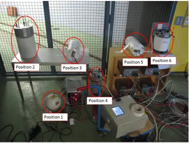
FIG. 23. Detectors installed in the six reference positions during the measurements performed at PS.
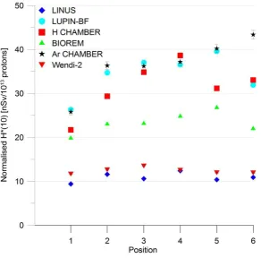
FIG. 24. Results of the intercomparison performed at PS in location 3, expressed as H*(10) normalised to the integrated proton fluence in the PS.
FIG. 25. Signal acquired with LUPIN-BF in location 3 at PS.
FIG. 26. Principle of the neutron/photon discrimination technique D1 applied in LUPIN.
FIG. 27. Signals acquired with LUPIN-He in both reference positions around the medical LINAC at
the San Raffaele hospital. The zoom of the first 15 μs shows the prompt photon peak.
FIG. 28. Signal acquired with LUPIN-BF at the test injector facility at PSI.
FIG. 29. Results obtained at HZB with LUPIN-BF expressed in measured and corrected H*(10) as a function of the reference value per burst. The linear response is represented by the black line.
FIG. 30. True and measured interaction rate as calculated for Wendi-2 for the measurements carried out
at HZB with machine setting 9.
FIG. 31. Comparison between the H*(10) measured by Wendi-2 and BIOREM at HZB for machine settings 1-12 and the H*(10) calculated via the analysis based on the neutron die-away time in the detector moderator.
8
FIG. 33. Signal acquired with LUPIN-BF at CNAO.
FIG. 34. The CNAO synchrotron lattice. The red marks show the 10 locations where LUPIN could be
installed to operate as BLM.
FIG. 35. Sketch of the SwissFEL injector test facility, with the 12 measuring positions shown on top
(BC = Bunch Compressor, BD = Beam Dump).
FIG. 36. Signal obtained with LUPIN-BF at PSI in reference position BC-back, dark current.
FIG. 37. Signal obtained with LUPIN-BF at PSI in reference position BC-back, normal operating
conditions.
FIG. 38. The CERN BSS: spheres, supports, detector, filler pieces and electronics.
FIG. 39. Geometry of the 81 mm sphere of the CERN BSS.
FIG. 40. Geometry of Ollio (right) and Stanlio (left) of the CERN BSS.
FIG. 41. Response functions calculated for the CERN BSS with the FLUKA code, expressed in counts
per unit of fluence as a function of the impinging neutron energy.
FIG. 42. Geometry of the 233 mm sphere of the BSS-LUPIN.
FIG. 43. Comparison between the response function obtained for the 81mm sphere for the CERN BSS
and for the BSS-LUPIN.
FIG. 44. Fixed beam treatment room at the proton therapy centre in Essen. The red spots indicate the
reference positions.
FIG. 45. Experimental set-up for the measurement performed with the 233 mm sphere in position 1a at
the Essen proton therapy centre.
FIG. 46. Neutron spectrum calculated for position 1a at the Essen proton therapy centre with MAXED,
GRAVEL and FRUIT, compared with the guess spectrum simulated via MNCPX.
FIG. 47. Neutron spectrum calculated for position 1b at the Essen proton therapy centre with MAXED,
GRAVEL and FRUIT, compared with the guess spectrum simulated via MNCPX.
FIG. 48. Neutron spectrum calculated for position 2a at the Essen proton therapy centre with MAXED,
9
FIG. 49. Experimental set-up for the measurements performed with the 178 mm sphere at the CERN
PS: BSS-LUPIN (left) and conventional CERN BSS (right).
FIG. 50. Spectrum calculated at PS for the measurements performed with the CERN BSS and the
10
List of abbreviations
The abbreviations are listed here in alphabetical order. Each acronym is also given in parentheses at the
first appearance of the full expression in the text.
ACCREDIA Italian National Centre for Accreditation
ADC Analogue to Digital Converter
BLM Beam Loss Monitor
BNC Bayonet Neill-Concelman
BSS Bonner Sphere Spectrometer
CERF CERN-EU Reference Field
CNAO Italian National Centre for Oncological Hadrontherapy
EURADOS European Radiation Dosimetry group
FEL Free Electron Laser
FPGA Field Programmable Field Array
HiRadMat High Radiation to Materials
HZB Helmholtz Zentrum Berlin
IC Ionisation Chamber
LINAC Linear Accelerators
LINUS Long Interval Neutron Survey Meter
LogAmp Logarithmic Amplifier
LUPIN Long Interval Ultra Wide Dynamic Pile Up Free Neutron Rem Counter
11
MSV Mean Square Voltage
M.U. Monitoring Units
PMMA Poly-Methyl Meth-Acrylate
PMT Photo Multiplier Tube
PNF Pulsed Neutron Fields
PS Proton Synchrotron
RAMSES Radiation Monitoring System for the Environment and Safety
rem Roentgen Equivalent Man
SCA Single Channel Analyser
SDD Single-crystal Diamond Detector
SPS Super Proton Synchrotron
SS Straight section
TTL Transistor-Transistor Logic
VELO Vertex Locator
12
1.
Introduction
1.1. Neutron detection
“These results, and others I have obtained in the course of the work, are very difficult to explain on the assumption that the radiation from beryllium is a quantum radiation, if energy and momentum are to be conserved in the collisions. The difficulties disappear, however, if it be assumed that the radiation consists of particles of mass 1 and charge 0, or neutrons [Chadwick 1932].” It took a while to the scientists of the first half of the nineteenth century to understand the characteristics of the
particle they were dealing with and to give it a proper name. Several hypotheses were made in order to
justify the presence of this very penetrating radiation that could not be easily stopped even in lead,
including the hypothesis made by Rutherford in 1920 [Rutherford 1920] and the theory that
Ambartsumjan and Iwanenko developed in 1930 [Ambartsumjan and Iwanenko 1930]. Only Chadwick
in 1932 speculated, and later proved, the existence of a neutral particle that allowed the energy and
momentum conservation laws to be still written in physics books without having to justify a
troublesome exception, and gave it the name of neutron. The late discovery of this particle if compared
to the discovery of electrons (1897) and protons (1919) was linked to the fact that it did not easily
interact and could not be easily stopped in matter. A direct consequence of this is that neutrons still
constitute the most difficult radiation field to be detected and stopped. Neutrons are usually detected
through nuclear reactions that result in prompt energetic charged particles such as protons, alpha
particles or heavier nuclides. The most common techniques involve the combination of a target material
designed to perform the conversion between neutron and a charged particle and another material in
which the charged particle can deposit at least a fraction of its energy. Since essentially all nuclear
reactions show an interaction probability, i.e. a cross section, whose value is maximum for low-energy
neutrons with a rapid decrease for increasing neutron energy, the target material is usually coupled with
a moderating material in order to reduce the energy of the impinging neutrons and then to increase the
interaction probability. The three most commonly employed nuclear reactions for thermal neutron
detection are listed below, whereas no indication is given on reactions induced by fast neutrons or on
methods employed to derive the neutron kinetic energy.
One of the most employed reactions for the detection of thermal neutrons is the 10B(n,α)7Li
13
to the ground state with a branching ratio of 6%, under the assumption that the reaction has been induced
by thermal neutrons. The Q-value of the reaction is 2.310 MeV or 2.792 MeV, depending on whether
the 7Li atom is produced in its excited or ground state, respectively. When it is produced in its excited
state, the 7Li atom returns with a half-life of 10-13 s to its ground state via the emission of a 480 keV
gamma ray. The Q-value is much higher than the energy of the incoming neutrons and therefore the
energy imparted to the reaction products is essentially equal to the Q-value itself. Similarly, as the linear
momentum of the impinging neutrons is negligible, the reaction products are emitted in exactly opposite
directions, and the energy is always shared between them in the same way, i.e. 0.84 MeV for the excited
7Li atom and 1.47 MeV for the α particle. The thermal cross section for this reaction is 3840 b, while
its value drops with increasing neutron energy, being proportional to the reciprocal of the neutron speed.
The popularity of this reaction comes not only from the high cross section value but also from the fact
that highly enriched boron is readily available.
Another reaction commonly employed for thermal neutron detection is the 6Li(n,α)3H reaction.
The 3H atom is produced only in the ground state and the reaction Q-value is 4.78 MeV. As for the 10B(n,α)7Li reaction, the Q-value is much higher than the energy of the impinging neutrons, and this
results in an energy transmitted to the reaction products which is essentially equal to the Q-value itself.
The 3H atom and the α particle are emitted in opposite directions with an energy of 2.73 MeV and
2.05 MeV, respectively. The reaction cross section for thermal neutrons is 940 b, with the usual decrease
for higher energy, which is proportional to the reciprocal of the neutron speed. Even if the 6Li(n,α)3H
reaction is characterised by a lower cross section than the 10B(n,α)7Li reaction, it has the advantage of
a higher Q-value, thus resulting in an easier discrimination of the neutron-induced events from the
electronics noise and the photon background. Moreover, as for 10B, also 6Li is readily available in
separated form.
The 3He(n,p)3H reaction is another reaction employed for detection of thermal neutrons. The
atom of 3H is produced in the ground state only and the reaction Q-value is 764 keV. The reaction
products are emitted in opposite directions with energy of 573 keV for the proton and 191 keV for the
3H atom. The thermal cross section is 5330 b, with the usual dependence on the reciprocal of the neutron
speed. 3He is a rare isotope of helium and, even if it is commercially available, its cost is relatively high
and in the last years a shortage of the 3He stocks occurred worldwide [Shea and Morgan 2010, Nuttall
14
of nuclear weapons and for many years its supply outstripped the demand, until the September 11th
attack, after which the U.S. government began deploying 3He neutron detectors at the borders for
homeland security. To face this problem, several solutions are being thought on how to increase the
production via other techniques and to reduce the demand by employing new technologies based on
different detection reactions. Nevertheless, since the situation nowadays seems to be partially improved,
for the studies performed in the framework of this thesis, it has been considered that the provision of
3He will still be possible at affordable prices in the next years.
Less than 20 years after the discovery of the neutron by Chadwick, the scientists started to
concentrate their efforts not only on the neutron detection techniques, which were developed in a
relatively short time, but also on the problems arising from the detection of neutrons in pulsed fields.
In fact with the development of the first particle accelerators it came clear that techniques had to be
developed in order to detect short pulses of radiation, both photons and neutrons, by limiting the
counting losses induced by the instrument dead time. Westcott was one of the pioneers in this research
field, since in one of his papers in 1948 he stated that “One of the outstanding trends in the present phase of research in nuclear physics is the use of increasingly large and complex machines for the acceleration of charged particles to very high energies… A feature common to all machines giving particles of the highest energies is that their output is not continuous, but occurs in bursts or pulses separated by relatively long intervals during which the machine gives no output… The difficulty which arises in electrical counting when the source is pulsed is due to the finite resolution of any counting system. Thus, following any count, there is a dead time during which the system would be unable to record a further count, should one occur [Westcott 1948].” In his long paper he tries to define several correction equations to compensate for these dead time losses based on several hypotheses and it ends
up with complex tables where one should find a correction factor to be applied to the instrument
readings in specific radiation conditions. This was the only way known at the time to limit the problem,
since no solutions existed on how to reduce the dead time under a certain value. This first investigation
triggered the interest of the scientific community, which ended up later on with numerous studies
focused on this topic. Section 1.2. explains the details of the problems in the present scientific context
15
1.2. Detection in pulsed neutron fields
The need of radiation detectors capable to measure efficiently in pulsed neutron fields (PNF)
is attracting widespread interest for applications such as radiation protection and beam diagnostics in
research and medicine particle accelerators. Since the 1960s, numerous investigations focused on the
development of detectors specifically conceived to work in pulsed fields. This is a major issue at particle
accelerators, where pulsed neutron and photon fields are present because of beam losses at targets,
collimators and beam dumps. The interest in active detectors to be employed in PNF is constantly
increasing due to the growing number of applications where the time structure of the stray neutron field
is characterised by a pulsed structure, i.e. by radiation bursts whose duration varies in a range from few
ns to few ms with a typical repetition rate in the range 0.1-100 Hz [Caresana et al. 2013c]. Among the
different applications we can find ultra-high intensity lasers, where a power varying from hundreds of
TW to a few PW is delivered onto a target in bursts whose duration is in the order of hundreds of fs
[Agosteo 2010], hadrontherapy facilities, characterised by a spill duration of 1 s and repetition rate of
about 0.5 Hz [Rossi 2011], material testing facility, spallation sources [Andersen et al. 2012], medical
linear accelerators (LINAC), laser plasma facilities and free electron lasers (FEL), where the accelerator
is usually operated at a repetition rate of 10 Hz and a bunch duration of a few ps [Pedrozzi 2010]. In all
these applications the pulsed structure of the radiation field hinders the use of active detectors operating
in pulse mode in the halls housing the accelerators and the beam lines, including the treatment rooms,
thus limiting their use in areas where the field intensity has been reduced and the typical duration of the
bursts increased. Therefore the choice is usually directed towards passive detectors, which show several
limitations, notably the fact that they cannot display the ambient dose equivalent, H*(10), rate in real time and that real time alarms cannot be set. Section 1.3 will describe the main limitations that affect
the performance of active detectors in PNF and the related causes.
Pulsed radiation usually consists of a sequence of short bursts, but also single bursts delivered
at low repetition rates are not uncommon. Though the H*(10) which characterises a single burst is usually low, and would not constitute a problem in terms of averaged H*(10) rate over the entire measurement period, the H*(10) rate during the radiation burst can reach extremely high values, up to 100 Sv/h in typical medical diagnostics applications and up to 107 Sv/h in facilities such as the ones
used for material testing [Schmidt et al. 2009], and this usually leads to severe underestimations of the
16
commercial active neutron detectors [Leake et al. 2010] with tremendous underestimation of the
H*(10), up to three orders of magnitude [Klett et al. 2007].
The main cause of this underestimation can be attributed to dead time losses, which are a
distinctive feature of active detectors working in pulse mode. An active radiation detector can in fact
operate in three modes: current, mean square voltage (MSV) and pulse mode. Current mode averages
out the fluctuations in the intervals between individual interactions and is usually employed with high
interaction rates when there is no need of preserving the information on the amplitude and timing of
single interactions. MSV mode, whose detection principle is based on a special processing of the
fluctuating component of the detector current signal, becomes useful when making measurements in
mixed radiation environments when the charge produced by one type of radiation is much different than
that from the second type. Pulse mode is the most commonly applied, especially for applications that
are better served by preserving information on the amplitude and timing of individual events. This is
the case for most neutron active detectors where the output usually consists of a sequence of individual
pulses, each representing the results of a single interaction. One of the advantages of pulse mode
operation is that the sensitivity is greater than when using current or MSV mode, because each
interaction can be detected as a distinct pulse. This is a desirable property for radiation protection
measurements because of the low detection limits required. The downside is represented by the dead
time losses induced by the counting system, which can be correctly compensated only in the case of
steady-state sources of constant intensity, but not in the case of pulsed sources. An ideal detector would
in fact count every event that occurs. However, a real detector and its read-out electronics need a
specific amount of time to create and process an output pulse. An event that occurs during this time
span cannot be registered correctly. Depending on the detector system, it is either suppressed (non
paralysable systems) or changes the shape of the previously detected pulse, resulting in a pile up
(paralysable systems). The minimal time between two separately detectable events is called the dead
time of the detector and the consequent losses are called dead time losses. The dead time for state-of
the-art neutron detectors typically ranges from 1 to 10 μs.
It is clear that an ideal active detector should not be affected by dead time losses if it has to be
employed in PNF. However, this is not the only constraint. One can define five other requirements that
an active neutron detector should show for efficiently working in PNF:
17
2) high sensitivity, usually expressed in nSv-1, at least comparable with that of commercially
available rem counters, i.e. about 1 nSv-1;
3) capability to measure correctly the intensity of a single neutron burst;
4) capability to reject the photon contribution that usually accompanies the neutron fields;
5) good sensitivity over the entire neutron energy range, especially to high-energy neutrons,
which is desirable for use in high-energy fields like those encountered around particle
accelerators or cosmic ray fields.
Section 1.3 gives a brief review of the active detectors available at the state of the art and of their main
limitations, with a special focus on the five requirements listed above.
1.3. State of the art detectors
One way to deal with the problem of the detection in PNF is to use activation detectors and
there has been extensive research in this field since the 1970s [Mayer and Brysk 1975, Slaughter and
Pickles 1979]. A considerable effort has recently been put on the improvements of silver activation
detectors [Dighe et al. 2004], for which experiments have shown good linearity of the response in PNF
[Luszik-Bhadra et al. 2010]. These detectors, however, show some limitations: they have a low neutron
sensitivity, i.e. about 9 μSv-1 for a bare 252Cf source [Luszik-Bhadra and Hohmann 2009], and they can
detect a neutron H*(10) of 10 μSv in a reliable way only if the photon contribution is a factor of 10 lower [Luszik-Bhadra et al. 2010]. However, the crucial issue is the response time, which is determined
by the half-life of the Ag isotope: the neutron capture (n,γ) on 107Ag and 109Ag produces 108Ag and 110Ag
isotopes, characterised by a half-life of 25 s and 144 s, respectively, which subsequently decay by β
-emissions in 108Cd and 110Cd. The approach based on silver activation detectors eventually fulfils the
requirements 1 and 4 given in Section 1.2, but does not permit the measurement of the intensity of a
single neutron burst. Moreover the sensitivity is about two orders of magnitude worse than
commercially available rem counters.
An alternative approach which relies on the activation of 12C has recently been proposed in a
new survey meter designed to work in PNF [Klett et al. 2010]. It detects neutron via the (n,pα), (n,x)
and (n,p) reactions on 12C and the resulting production of 8Li, 9Li and 12B isotopes, which subsequently
decay by β- emissions in 8Be, 9Be and 12C. The decay process is fast, being characterised by a half-life
18
This means that the instrument has limited applications as it can only be used for detecting with good
efficiency neutrons above 20 MeV, and has strong limitations in sensitivity and on the burst repetition
rate over which it can be used [Leake et al. 2010]. Consequently, the requirements 1 and 2 cannot be
fulfilled.
Single-crystal diamond detectors (SDD) have been used effectively in PNF [Rebai et al. 2012].
Diamond is characterised by one of the highest atomic density and allows an SDD to have very high
radiation efficiency per unit of volume and, consequently, extremely compact dimensions. The high
mobility of the charge carriers leads to a very fast response, which minimizes the dead time losses,
provided that the SDD is coupled to special fast amplifiers. The fast neutron detection is based on the
(n,α), (n,p) and (n,d) reactions on 12C which produce 9Be, 12B or 11B. However, these detectors are
sensitive only to high-energy neutrons, above a few MeV, and must be coupled with 6LiF or 10B in order
to detect thermal neutrons, but this would increase the complexity of the detector and alter the fast
response properties.
A different approach which is using a proportional counter connected to a conventional
acquisition chain has recently been proposed in order to reduce the counting losses in PNF [Weizhen et
al. 2009]. This method takes into account the nearly simultaneous detection of two or three neutrons,
which are discriminated by the single interaction event and which generate a double or triple logic
signal at the output of the single channel analyser (SCA). However, this method proved to be reliable
up to a limit of 100 counts generated by a single burst in the detector and a limit of 0.1 Gy/h on the
photon H*(10) rate that accompanies the neutron field. The limit on the number of counts is very stringent and does not allow the detector to meet the requirements 1 and 3.
A promising theoretical method which allows dealing with the typical problems of the
detection in PNF has recently been proposed [Leake et al. 2010]. It is based on the exploitation of the
die-away of thermalised neutrons in the detector moderator: when a large neutron burst is detected, the
interaction rate is initially too high to be correctly detected but then it exponentially decays and, after a
certain time, it falls below a certain level where the dead time losses become negligible. If a proper
algorithm is implemented in the detector acquisition system, then the size of the initial burst can be
calculated by measuring the tail of the signal, i.e. by measuring the integrated number of detected
19
method, which will be further investigated in Section 2.4, but at present it has not been put into practice
in any detector acquisition system.
Recently a new neutron monitor has been designed to measure the H*(10) rate of high intensity neutron bursts generated by beam losses in an accelerator [Iijima et al. 2011]. This detector is based on
a current readout and shows no count losses in a dynamic range from 4 μSv/h to 5 mSv/h. The drawback
of the current working mode is that the monitor cannot distinguish a signal generated by a photon and
a neutron and it cannot preserve the information on the amplitude and timing of the single interactions.
It cannot therefore operate under stringent constraints and the requirements 1 and 4 cannot be respected.
This brief review showed that at the state of the art there is no device capable of fulfilling all
the requirements listed in Section 1.2 for efficiently measuring in PNF. A new approach is treated in
this thesis: an innovative detection principle, based on logarithmic amplification, and subsequent
integration, of the current signal collected at the output of a proportional counter, is applied as the main
operating principle of the detection devices: an extended range rem counter, a beam loss monitor (BLM)
and an extended range Bonner Sphere Spectrometer (BSS). Chapter 2 describes the rem counter, its
working principle, the results of measurements performed in various stray field conditions, and goes
into the details of some aspects of the detector physics; Chapter 3 describes the working principle of
the BLM, the measurements performed and the basic principles of its implementation in an machine
protection system; Chapter 4 describes the physical characteristics of the BSS, the procedure followed
to calculate the response of each sphere as a function of the impinging neutron energy, and the
measurements carried out in different radiation environments. The conclusions are given in Chapter 5,
together with the lists the possible applications of the innovative instrumentation described in this thesis
20
2.
LUPIN, an innovative rem counter
This chapter describes an innovative rem counter called Long interval Ultra-wide dynamic
Pile-up free Neutron rem counter (LUPIN) and the measurement campaigns performed to test and
improve its performance. The term rem counter is used as an inheritance of past decades, when the first instruments capable of directly relating the results of the measurements with the corresponding neutron
equivalent dose were called Roentgen equivalent in man (rem) counter or rem meter, with a direct
reference to the measuring unit of the time. These detectors should be called nowadays H*(10) counters. However, the old acronym is still widely used in radiation protection to define all instruments based on
a thermal neutron detector and on a moderating assembly capable of directly relating the number of
measured counts with the neutron H*(10). Therefore the term rem counter has been used throughout the text to define LUPIN and similar instruments. Section 2.1. describes the main characteristics and
the working principle of this innovative rem counter. Section 2.2. reports the description and the results
obtained in several measurements campaigns in which the detector has been tested to verify its
performance and to understand its possible applications and limitations. Section 2.3. discusses the origin
and the consequences of the space charge effect which is the main cause of the limitations observed in
the detector when it is exposed to extremely intense PNF. Section 2.4. is focused on the experimental
evidence of the presence of a neutron die-away time characteristic of any thermal neutron detector such
as LUPIN and on the proposal of an innovative acquisition technique based on this die-away time which
should be in principle applicable to any neutron detector working in pulse mode.
The aim of the measurement campaigns described in this chapter was to test the detector in the
most different stray field conditions in order to analyse its in the field performance and to derive useful information from each test in order to implement changes in its physical characteristics, in the
acquisition interface and in the off-line analysis techniques. This allowed optimizing the detector
performance in parallel while continuing planning new measurement campaigns, thus drastically
reducing the time required to reach the actual development, i.e. a prototype with robust reliability and
21
All measurements have been performed in the framework of my thesis work. Similarly, the
data shown in the tables and in the figures, as well as the results at which the text indirectly refers, have
been obtained during the work carried out in the PhD, opportunely supported by technicians, physicists
and other colleagues, and under the close monitoring of the university supervisor. Where the discussion
or the conclusions refer to measurements or data that have not been obtained by me personally, the text
clearly refers to external sources, such as papers, conference proceedings, books or internal reports. In
this latter case, since the reader could find difficulties in obtaining the original text, the bibliography
reports, close to the standard reference formula, an hyperlink whose validity has been verified in May
22
2.1. The detector
LUPIN is a rem counter type instrument available in two versions, consisting of either a 3He
or a BF3 proportional counter placed inside a spherical or cylindrical moderator, respectively. From
now on, for simplicity, the text will refer to LUPIN-He and LUPIN-BF, respectively. The moderator is
designed so that the response function of the instrument reproduces sufficiently well the curve of the
conversion coefficients from neutron fluence to H*(10) over a wide energy range, as in the original extended range Long Interval NeUtron Survey meter (LINUS) [Birattari et al. 1990, Birattari et al.
1992, Birattari et al. 1993, Birattari et al. 1998].
The LUPIN-He moderator consists of a polyethylene sphere of 12.5 cm outer radius with lead
and cadmium inserts, hosting at its centre the 3He. The inner part of the moderator, 5.6 cm in radius, is
surrounded by a 6 mm thick lead shell. The outer layer of this inner polyethylene sphere hosts eleven
cadmium buttons, 2.5 cm in radius and 1 mm thick. Polyethylene fillers are used to fill the void around
the detector stem. A scheme and a photograph of the inner parts of LUPIN-He are shown in Fig. 1.
FIG. 1. Scheme and photograph of the inner parts of LUPIN-He, dimension in centimetres.
The same moderator has been used with CR-39 dosimeters and a 3He proportional counter as a
dual-detector extended range rem counter by Agosteo et al. [Agosteo et al. 2010]. The difference here is the
presence of the electrostatic shielding that contains the detector and the polyethylene inserts, which is
constituted by an aluminium cylinder of 1.5 mm thickness. In order to host this cylinder, the diameter
of the polyethylene fillers was reduced by 3 mm.
The LUPIN-BF moderator consists of a polyethylene cylinder of 25 cm diameter with lead
23
the one used in the spherical moderator, i.e. 1.5 mm, but it is longer due to the bigger length of the BF3
and of the polyethylene fillers. A scheme and a photograph of LUPIN-BF are shown in Fig. 2.
FIG. 2. Scheme and photograph of the moderating assembly of LUPIN-BF, dimensions in centimetres.
The proportional counters used in the two versions of LUPIN are a spherical Centronic
SP9He3/152/Kr 3He and a cylindrical Centronic 15EB/20/25SS BF
3, characterised by a nominal
pressure of 1520 mmHg (203 kPa) and 200 mmHg (267 kPa), respectively. However, even if the
pressure of the 3He is nominally stated as 1520 mmHg (203 kPa), the actual pressure is 1748 mmHg
(233 kPa), to which 912 mmHg (122 kPa) of Krypton is added as a quench gas [Sutter 2011].
The front-end electronics consists of a current-voltage logarithmic amplifier, whose output
signal is acquired by an analogue to digital converter (ADC) with a conversion rate of 10 MSamples/s
and processed with a LabVIEW program running on a PC. The idea at the basis of the software is
simple: the voltage signal is converted back into a current signal and integrated over a time that can be
freely set by the user. The result of this calculation represents the total charge generated in the detector
by the neutron interactions. This quantity, divided by the average charge expected by a single neutron
interaction, represents the number of interactions occurring during the integration time. The acquisition
may start when the current signal overcomes a certain threshold, via the so called trigger mode, or at regular intervals, regardless of what the current value is, via the streaming mode. The first acquisition mode allows the user to focus its attention to the shape of the signal and guarantees that the data are not
integrated in case of absence of neutron interactions. For most of the measurement campaigns this mode
24
certain area, the streaming mode must be employed; otherwise the measured value would overestimate the actual one.
The scheme of the front-end electronics is shown in Fig. 3.
FIG. 3. Schematic working principle of the LUPIN electronics.
The polarisation between the electrodes of the proportional counter is provided by a user-adjustable
internal high voltage supply. The electronics is based on a current-voltage logarithmic amplification of
the signal produced inside the proportional counter. A fixed current Imin is added to the current signal
IR generated by the reactions inside the gas to avoid negative saturation in case of absence of signal
generated by the neutron interactions. The current Imin is usually set to 160 pA, but this value can be
modified if necessary. A larger value of Imin induces a faster response of the logarithmic amplifier
(LogAmp). The sum of the two currents, IR + Imin, is collected and processed by the LogAmp. Even if
the value of Imin is negligible for typical acquisition conditions, it plays a role when the detector is used
to measure radiation background. Therefore proper techniques are put in place in order to subtract the
charge generated by this very low current from the total charge, see Section 2.2.6. The proportional
counter must be electrostatically shielded to avoid noise pick up. The electrostatic shield is constituted
by an aluminium cylinder that encases the detector, as discussed above. The LogAmp output signal
passes through a cable driver and the signal VLogOut is acquired via a PC digital oscilloscope
(Picoscope™ 4424 by PicoTechnology) and monitored by the LabVIEW program. The choice of a
LogAmp was driven by the need to achieve a dynamic range of a few orders of magnitude with respect
to the burst intensity to be measured. Conventional LogAmps are too slow for the purpose of the
25
time constants when they are fed with low currents, and this is usually the case during the detection of
the tail of the signal. It was then decided to employ a high-speed LogAmp, i.e. the Texas Instruments
LOG114. The LogAmp is declared to work over a range of eight decades (160 dB) with high
temperature stability. The circuital scheme of the front-end electronics is shown in Fig. 4.
FIG. 4. Circuital scheme of the LUPIN electronics.
The principle of detection of LUPIN differs strongly from the ones employed by most active neutron
detectors. It introduces in fact a big simplification in the overall acquisition chain. In a conventional
detector working in pulse mode the signal generated in the proportional counter first needs to be
pre-amplified before the main stage of amplification, and then needs to pass in an SCA in order to be
discriminated from electronic noise and interactions of other particles, such as photons, in the detector.
Eventually, a counter must be employed to display the total number of detected neutron interactions. In
LUPIN, the signal is directly fed to the amplifier, and the number of neutron interactions is derived
from the total integrated charge. The main advantage of this principle of detection is that the system is
not affected by dead time losses, which are usually introduced by the SCA. The dead time losses can
induce severe underestimations of the true interaction rate, as it has been explained in Section 1.2. For
example a dead time of 5 μs, which is typical of a rem counter, leads to an underestimation of 50% at a
true interaction rate of 2∙105 s-1, assuming that the acquisition electronics can be treated as a
non-paralysable system [Knoll 2010b].
Both versions of LUPIN show some advantages and some drawbacks as well. The choice of
the version should be driven by the type of application and by the characteristics of the stray radiation
26
higher Q-value of the 10B(n,α)7Li reaction if compared to the 3He(n,p)3H which results in a
better photon rejection and, consequently, a better neutron/photon discrimination;
larger active volume, 25 mm diameter and 150 mm length for the BF3, to be compared with
the 31 mm diameter for the 3He, which reflects in a mitigation of the space charge effect. This
effect is generated when a large number of neutron interactions occur in the gas in a very short
time: the space charge causes a reduction in the electric field around the anode and
consequently a decrease in the multiplication factor. Its importance is therefore reduced if
larger active volumes are employed [Rios et al. 2013]. A complete discussion on this topic, as
well as on the possible countermeasures that can be put in place to limit its consequences, will
be given in Section 2.3.
On the other hand, the advantages of LUPIN-He are:
higher sensitivity, which is a direct consequence of the higher pressure and the higher
multiplication factor of the 3He compared to the BF 3;
isotropic response, due to the spherical geometry of the proportional counter and the
moderating assembly.
2.2. Measurements
The development of LUPIN was performed in parallel with the execution of tests and
measurement campaigns. This allowed a continuous and progressive development of the detector and
a consequent optimisation of its characteristics. Therefore the results obtained in the measurements and
in the intercomparison campaigns will be presented by including at the end of each section the key
information derived from each series of test, the limitations and the problems encountered, as well as
the solutions implemented to solve them. The facilities where the detector has been employed were
chosen in order to test LUPIN in most different radiation environments, ranging from a calibration
laboratory to operational conditions around particle accelerators and extreme situations where the
detector was brought to its limits of operation, reproduced on purpose in dedicated facilities or research
centres. For each section a description of the facility and the expected stray field conditions is given,
together with an overview of the radiation detectors employed. In many cases the measurements were
carried out in the framework of larger intercomparisons or wider collaborations. In this case the
27
the main specifications and the response functions of the detectors used for comparison in the different
measurements are given in Appendix: throughout the section the detectors will be referred only with
their commercial acronyms.
2.2.1. Detector calibration
The characterisation of LUPIN is connected to its working principle and requires the
knowledge of two calibration factors, instead of the single calibration factor usually needed for a rem
counter: the mean collected charge (MCC), expressed in fC, i.e. the average amount of charge generated
in the detector by a neutron interaction. This is used to derive the number of neutron interactions
occurring during the integration time, and the conversion coefficient from neutron interactions to
H*(10), expressed in nSv-1. The measurements were performed with calibrated neutron sources in two
dedicated laboratories, at the Politecnico di Milano and at CERN.
The calibration in charge was performed in the calibration laboratory at the Politecnico di Milano with an AmBe source. Knowledge of the precise activity of the source is not an essential value for these measurements, since the only requirement is to have one, and only one, neutron interaction in
each acquisition. The source-detector distance was therefore tuned in order to obtain about 10 s-1
interactions, a rate low enough to avoid multiple interactions in a single acquisition, but sufficiently
high to limit the time needed to reach a reasonably low statistical uncertainty on the integrated number
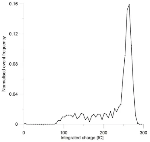
of counts, i.e. less than 1%. Several integration times where used, ranging from 0.5 ms to 4 ms. Fig. 5
and Fig. 6 show the distributions for both versions of LUPIN, where the frequency of events for each
bin has been normalised in order to set the sum of all the data to 1. The noise-induced low-energy events
have been excluded from the plot: the full-energy deposition peak and the wall effect continuum are
clearly visible. The wall effect is the direct consequence of the fact that the incoming neutrons carry no
appreciable momentum. Therefore, the products of the neutron-induced reaction, 3H and p in the case
of 3He, 7Li and α in the case of BF
3, are emitted in opposite directions and the reduced dimensions of
28
FIG. 5. Normalised distribution of the charge integrated with LUPIN-He over a 4 ms acquisition time.
FIG. 6. Normalised distribution of the charge integrated with LUPIN-BF over a 4 ms acquisition time.
The MCC is defined as the weighted average of the charge distribution, after having set a proper upper
and lower limit in order to cut the electronics noise and the energy depositions due to photon interactions
in the gas. It depends on the detector, the operating voltage and the integration time, as shown in Table I:
it reaches a plateau for integration times longer than 1 ms. For lower values the charge collection is incomplete due to the ballistic deficit, i.e. the difference in the amplitude of the pulse if compared to
[image:31.595.194.443.345.580.2]29
uncertainty in the determination of the MCC is due to the statistical uncertainty on the integrated number
of counts.
Table I. Values of MCC as calculated for several integration times.
Integration time [ms] MCC [fC]
LUPIN-He LUPIN-BF
0.5 211 ± 15 547 ± 38
1 229 ± 16 616 ± 43
2 243 ± 17 611 ± 43
3 251 ± 18 616 ± 43
4 260 ± 18 617 ± 43
The calibration in H*(10) was performed in the CERN calibration laboratory with a PuBe source. The integration time was set to 2 ms. The calibration factor was determined to be
2.13 ± 0.17 nSv-1 for LUPIN-BF and 3.64 ± 0.26 nSv-1 for LUPIN-He. In order to test the geometrical
dependence of the response of LUPIN-BF, which is not isotropic due to the cylindrical shape of the
moderating assembly, the calibration was also performed at different angular orientations, along the
three detector axes, see Fig. 7.
FIG. 7. Configurations used to test the geometrical dependence of LUPIN-BF. The red arrow indicates the positive direction of angular turning.
The detector has been turned in different orientations by steps of 30˚, from -150˚ to +180˚, in each of
the three configurations. The results are shown in Fig. 8, where the uncertainties are not displayed for
clarity. The total uncertainty is the sum of the statistical uncertainty on the integrated number of counts
and the uncertainty on the calibration of the neutron source, i.e. 7%, as obtained from the source
30
FIG. 8. H*(10) calibration factor obtained for different orientations of LUPIN-BF along the three axes. As expected, the response is not isotropic. However, the difference in the value of the calibration factor
is always included in a ±20% variation, for all orientations along the three axes. This variation can be
further limited if a BF3 counter characterised by a lower active length is employed. Under this condition
the height of the moderating assembly could be slightly reduced so that it would become approximately
equal to the cylinder diameter, in order to resemble a quasi-isotropic geometry. However a lower active
length of the proportional counter would result in reduced detector sensitivity.
2.2.2. Measurements in high-energy mixed fields
Measurements were carried out at the CERN-EU high-energy reference field (CERF) facility
[Mitaroff and Silari 2002] to test the performance of LUPIN-BF in high-energy mixed fields. The
facility was conceived to generate a stray radiation field which resembles the high-energy component
of the radiation field created by cosmic rays at commercial flight altitudes. Although the detector is
specifically conceived for PNF, a test in operational non-pulsed conditions is necessary. This is in fact
a typical stray field that can be found not only at commercial flight altitudes but also close to the
shieldings of high-energy particle accelerators, where LUPIN could be employed as an on-line radiation
monitor for machine and personnel protection.
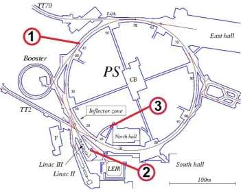
The CERF facility is installed in one of the of the secondary beam lines (H6) of the Super
Proton Synchrotron (SPS) in the North Experimental Area on the Prévessin site of CERN. The stray
31
4% kaons) with momentum of 120 GeV/c impinging on a copper target, 7 cm in diameter and 50 cm in
length, placed inside an irradiation cave, see Fig. 9.
FIG. 9. Axonometric view of the CERF facility. The side shielding is removed to show the inside of the irradiation cave with the copper target set-up.
The secondary particles produced in the target traverse an 80 cm concrete shield on top. This roof shield
produces an almost uniform radiation field over an area of 2 x 2 m2 located at approximately 90º with
respect to the incoming beam direction, divided in 16 squares of 50 x 50 cm2. Each element of this grid
represents a reference exposure location (concrete top, CT). The energy distribution of the particles,
mainly neutrons, at the various exposure locations were obtained in the past by Monte Carlo simulations
performed with the FLUKA [Ferrari et al. 2005, Battistoni et al. 2007] code. The neutron spectrum
outside the concrete shielding is dominated by a peak at 100 MeV, a smaller evaporation peak at about
1 MeV and a low-energy tail due to backscatter radiation. The beam is delivered to the CERF facility
from the SPS with a typical intensity of 108 particles per SPS spill. The spill duration, i.e. the beam
extraction time, varies along the years but during the measurements was equal to about 10 s over an
SPS cycle of 48 s.
The beam monitoring was provided by an air-filled, parallel-plate, transmission type ionisation
chamber (IC), which has been calibrated via the foil activation technique using the 27Al(p,3pn)24Na and natCu(p,x)24Na monitor reactions [Ferrari et al. 2014]. The beam intensity measured by the IC was
recorded every second in a log-file. The intensity is expressed in IC counts, since a current to frequency
converter allows the output current to be converted in Transistor-Transistor Logic (TTL) signals, which
32
The foil activation experiments confirmed the validity of the calibration factor used in past years: 1 IC
count corresponds to 22,000 ± 2,200 primary particles. The reliability of this value has also been
verified via FLUKA simulations carried out in order to obtain the expected charge collected on the
plates of the IC per primary particle. This allowed an extrapolated calibration factor of
22,172 ± 2,200 primary particles per IC count to be obtained, in excellent agreement with the value
obtained via the foil activation experiment.
The measurements were performed by installing in turn LUPIN-BF in the 16 reference
exposure locations on top of the concrete shield. Fig. 10 shows an example of the measurement set-up,
where several detectors are exposed on the concrete roof.
FIG. 10. Experimental set-up on the CERF concrete top shield.
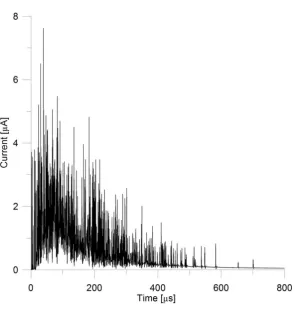
The integration time of LUPIN-BF was set to 10 s in order to be synchronised with the SPS spill
33
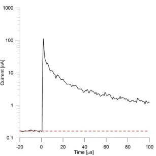
FIG. 11. Signal acquired with LUPIN-BF in the reference location CT16 at CERF.
The duration of the signal is equal to the spill duration of the SPS, i.e. about 10 s. The stray field is
characterised by a huge number of current peaks very close one to the other, which result in an almost
constant level of current throughout the entire spill. Each of the current spikes represents a neutron
interaction in the detector and in some cases they represent pile upping interactions, which give rise to
current peak up to 950 nA, clearly emerging in the signal. However, it cannot be excluded that some of
the peaks have been generated by interactions of high-energy particles in the detector, which directly
ionised the active gas or which resulted in a scattering event of atoms constituting the detector walls,
which later deposited their energy in the gas. The results were obtained by integrating the H*(10)
measured by LUPIN-BF in 15 minutes and by normalizing it to the integrated beam fluence, as obtained
from the log files of the beam monitor, expressed in IC counts. These results were compared with the
34
Table II. Results of the measurements performed with LUPIN-BF in the CT reference locations at CERF, compared with the results derived from FLUKA simulations (uncertainty in parentheses).
Location CT1 CT2 CT3 CT4 CT5 CT6 CT7 CT8
LUPIN-BF (nSv/IC count)
168 (51)
203 (61) n.a.
177 (53) 175 (53) 224 (67) 227 (68) 197 (59) FLUKA (nSv/IC count) 216 (22) 254 (25) 253 (25) 207 (21) 225 (23) 270 (27) 270 (27) 222 (22) Ratio LUPIN-BF/FLUKA 78% (8) 80% (8) n.a.
86% (9) 78% (8) 83% (9) 84% (9) 89% (9)
Location CT9 CT10 CT11 CT12 CT13 CT14 CT15 CT16
LUPIN-BF (nSv/IC count) 169 (51) 220 (66) 232 (70) 199 (60) 149 (45) n.a.
193 (58) 167 (50) FLUKA (nSv/IC count) 213 (21) 267 (27) 265 (27) 207 (21) 190 (19) 223 (22) 221 (22) 182 (18) Ratio LUPIN-BF/FLUKA 79% (8) 82% (9) 88% (9) 96% (10) 78% (8) n.a.
87% (9)
92% (10) n.a. = not available
The uncertainty on the measurements is due to the statistical uncertainty on the number of integrated
counts and to the uncertainty on the reproducibility of the positioning, i.e. 2%, equal to 1/10 of the
maximum difference between the reference value of H*(10) in a specific location and the adjacent ones. Since FLUKA simulations give a result that is normalised to the primary particles, the derived values
have an uncertainty which is equal to the uncertainty on the calibration of the beam monitor, i.e. 10%.
There is a very good agreement between experimental and Monte Carlo results, though for
some locations LUPIN-II slightly underestimates the H*(10). This underestimation reaches 15-20% for the locations placed on the left side of the concrete top, by taking as reference the picture shown in
Fig. 10. This slight difference has been noticed in a similar experiment carried out with other rem
counters in the same conditions and could be due to slight imprecisions of the geometry implemented
in the FLUKA simulations, especially for what concerns the target position in the irradiation cave, as
well as to the fact that the actual calibration factor of LUPIN-BF is higher when the stray field is
reaching the detector from the bottom side, see Section 2.2.1.
The results obtained with LUPIN-BF in position CT7 were compared with the results obtained
by other rem counters and neutron detectors in the same reference position. The detectors employed in
35
conventional and extended range rem counters: LINUS, LB6411, Wendi-2 and BIOREM,
whose response to neutrons can be enhanced by adding an external lead shell;
other neutron detectors: RadEye™, in the 3He version, employed with its small-size
polyethylene moderator to increase the efficiency to fast neutrons, and the ABC 1260 neutron
dose-meter, a bubble detector using an active counting system, whose response can be
extended to several hundred MeV with the addition of a 1 cm thick cylindrical lead shell placed
around the detector cap.
The results are shown in Fig. 12.
FIG. 12. Comparison between the H*(10) measured at CERF, grouped in detector classes: extended range (left) and conventional rem counters (centre), bubble detectors (right). The FLUKA value is also shown, together with the ±1σ (dashed line) and ±2σ deviations (dotted line).
The results obtained with the extended range rem counters, which include LUPIN-BF, are in good
agreement within the range of uncertainties and agree within 1σ with the value obtained by FLUKA.
The readings of the conventional rem counters are in good agreement within their uncertainties and
underestimate H*(10), as measured by the extended range instruments and as calculated by FLUKA, by about 40%. This is due to the reduced sensitivity of these detectors for neutrons with energies
>10 MeV. The ABC detector behaves like a conventional rem counter when it is employed without the
lead cap, otherwise its results are compatible with the extended range rem counters. The result of
RadEye™ has been excluded from the plot because it overestimates the FLUKA value by more than a
36
LUPIN-BF showed results in terms of integrated H*(10) which are compatible with what has been obtained by FLUKA simulations and by other extended range neutron detectors. Its reliable
behaviour in high-energy fields derives from the fact that its response closely resembles the ICRP
conversion curve from neutron fluence to H*(10). The lead parts included in the detector assembly help improving its sensitivity above 20 MeV by spallation reactions of the type (n,xn) induced by
high-energy neutrons. The multiple neutrons generated in these reactions are subsequently thermalised by
polyethylene and diffuse until they reach the active part of the detector, thus improving its response.
The small deviation of the measured from the simulated H*(10) for a few reference positions can be explained by the different calibration factor that should be applied to LUPIN-BF when it is exposed in
a neutron field directed from the bottom to the top part of it. This variation of the calibration factor
cannot be easily implemented and is due to the non-isotropic response of cylindrical neutron detectors.
This issue could be partially resolved by reducing the height of the detector, thus trying to approach a
quasi-spherical geometry. This could be done in two ways: by reducing the amount of polyethylene
below the proportional counter or by reducing the active length of the proportional counter. However,
if this would limit from one side the geometrical dependence of the calibration factor, it would add
other limitations: a lower amount of polyethylene would consistently reduce the detector sensitivity for
fast neutrons; moreover a reduced active length of the proportional counter would result in a reduced
sensitivity in the entire neutron energy range. In conclusion, the measurement campaign confirmed the
possibility of efficiently employing LUPIN in non-pulsed high-energy mixed fields, such as the one
encountered around high-energy accelerators or in aircrafts at commercial flight altitudes.
2.2.3. Measurements in a reference pulsed field
A series of measurements was performed with both versions of LUPIN at the
Helmholtz-Zentrum Berlin für Materialen und Energie GmbH (HZB) to test its performance in a reference pulsed
neutron field of increasing intensity. The aim was to evaluate the linearity of the response of the
detector, which was installed in a reference position 50 cm downstream of a tungsten target, as a
function of the radiation burst charge impinging on it. The measurements were performed in the
framework of a large intercomparison campaign organised by the Working Group 11 of the European
Radiation Dosimetry Group (EURADOS), whose research is primarily focused on dosimetry in
37
The cyclotron used for the measurements is routinely employed for proton therapy of ocular
tumours but, in addition to therapy, a small number of experiments for radiation hardness tests, detector
tests and dosimetry are also performed. The beam line directed towards the treatment room, shown in
Fig. 13, is equipped with a switching magnet that supplies the ion beam to the experimental room used
for the measurements.
FIG. 13. The cyclotron complex at the HZB.
A 68 MeV proton beam accelerated by the cyclotron impinged on a 20 mm thick tungsten target. The
choice of the target material was driven by the need of having the largest possible production of neutrons
generated in spallation reactions from the primary beam. Therefore a high-Z material as tungsten, which
is readily available, has been chosen. For treatment purposes the accelerator works in quasi-DC mode,
whereas for this measurement campaign the proton beam was delivered in bursts by using a burst
suppressor between the Van de Graaff injector and the cyclotron. The burst suppressor deflects the
beam and sends it to the target only for the desired time. This technique allows generating radiation
bursts with a time duration ranging from 50 ns to 1 ms with a maximum repetition rate of 100 kHz,
whereas the beam current can vary between 0.5 pA and 300 nA. The possibility of varying these