Roche tomography of cataclysmic variables - I. Artefacts and techniques

Roche tomography of cataclysmic variables – I. Artefacts and techniques

C. A. Watson

and V. S. Dhillon

Department of Physics and Astronomy, University of Sheffield, Sheffield S3 7RH

Accepted 2001 February 2. Received 2001 January 3; in original form 2000 October 16

A B S T R A C T

Roche tomography is a technique used for imaging the Roche-lobe-filling secondary stars in cataclysmic variables (CVs). In order to interpret Roche tomograms correctly, one must determine whether features in the reconstruction are real, or the result of statistical or systematic errors. We explore the effects of systematic errors using reconstructions of simulated data sets, and show that systematic errors result in characteristic distortions of the final reconstructions that can be identified and corrected. In addition, we present a new method of estimating statistical errors on tomographic reconstructions using a Monte Carlo bootstrapping algorithm, and show this method to be much more reliable than Monte Carlo methods which ‘jiggle’ the data points in accordance with the size of their error bars.

Key words: line: profiles – binaries: close – stars: imaging – stars: late-type – novae, cataclysmic variables.

1 I N T R O D U C T I O N

The secondary, Roche-lobe-filling stars in CVs are key to our understanding of the origin, evolution and behaviour of this class of interacting binary. To best study the secondary stars in CVs, we would ideally like direct images of the stellar surface. This is currently impossible, however, as typical CV secondary stars have radii of 400 000 km and distances of 200 pc, which means that to detect a feature covering 20 per cent of the star’s surface requires a resolution of approximately 1 microarcsecond, 10 000 times greater than the diffraction-limited resolution of the world’s largest telescopes. Rutten & Dhillon (1994) described a way around this problem using an indirect imaging technique called

Roche tomography which uses phase-resolved spectra to reconstruct the line intensity distribution on the surface of the secondary star.

Obtaining surface images of the secondary star in CVs has far-reaching implications. For example, a knowledge of the irradiation pattern on the inner hemisphere of the secondary star in CVs is essential if one is to calculate stellar masses accurately enough to test binary star evolution models (see Smith & Dhillon 1998). Furthermore, the irradiation pattern provides information on the geometry of the accreting structures around the white dwarf (see Smith 1995). Perhaps even more importantly, surface images of CV secondaries can be used to study the solar – stellar connection. It is well known that magnetic activity in isolated lower main-sequence stars increases with decreasing rotation period (e.g. Rutten 1987). The most rapidly rotating isolated stars of this type have rotation periods of,8 h, much slower than the synchronously rotating secondary stars found in most CVs. One would therefore

expect CVs to show even higher levels of magnetic activity. There is a great deal of indirect evidence for magnetic activity in CVs – magnetic activity cycles have been invoked to explain variations in the orbital periods, mean brightnesses and mean intervals between outbursts in CVs (see Warner 1995). The magnetic field of the secondary star is also believed to play a crucial role in angular momentum loss via magnetic braking in longer period CVs, enabling CVs to transfer mass and evolve to shorter periods. One of the observable consequences of magnetic activity are star-spots, and their number, size, distribution and variability, as deduced from surface images of CV secondaries, would provide critical tests of stellar dynamo models in a hitherto untested period regime.

However, determining whether features in Roche tomography reconstructions are real or not is problematic, as the resulting maps are prone to both systematic errors, due to errors in the assumptions underlying the technique, and statistical errors due to measurement errors on the observed data points. It is therefore essential to quantify the effects of these errors on Roche tomograms in order to properly assess the reality of any features present. In this paper we study the artefacts produced by errors in the input parameters using reconstructions of simulated data sets, and present a technique for estimating the statistical errors on the reconstructions. Subsequent papers will present the application of Roche tomography to real data sets.

2 R O C H E T O M O G R A P H Y

Roche tomography (Rutten & Dhillon 1994, 1996) is analogous to the Doppler imaging technique used to map rapidly rotating single stars (e.g. Vogt & Penrod 1983), detached binary stars (Ramseyer, Hatzes & Jablonski 1995) and contact binaries (Maceroni et al. 1994). However, in contrast to the Doppler P

imaging technique, the continuum is ignored in Roche tomography because of the unknown and variable contribution of the accretion regions to the spectrum, which forces Roche tomography to map absolute line fluxes. Apart from this, the principles differ only in detail.

Each tile or surface element is assigned a copy of the local (intrinsic) specific intensity profile convolved with the instrumental resolution. These profiles are scaled to take into account the projected area, limb darkening and obscuration, and then Doppler-shifted according to the radial velocity of the surface element at a particular phase. Summing up the contributions from each

element gives the rotationally broadened profile at that particular orbital phase.

not change. This iterative procedure is carried out (assuming no contribution from the accreting regions) until a satisfactory fit to the observed data, defined by the x2 statistic (i.e., x2_{,1Þ, is} achieved. As there are a large number of different intensity distributions that all predict trailed spectra consistent with the observed one, an additional constraint is required. This is found by selecting the map of maximum entropy with respect to a suitable default map, and is performed using the maximum-entropy algorithm developed by Skilling & Bryan (1984). Further details on the Roche tomography process can be found in Dhillon & Watson (2001).

3 S Y S T E M AT I C E R R O R S A N D A R T E FA C T S

There have been a number of studies exploring the effects of systematic errors on Doppler images of single stars. For example, the significance of so-called polar spots (large, long-lived, high-latitude spots straddling the polar regions) has been tested for robustness against errors such as incorrect line profile models (Unruh & Collier Cameron 1995), chromospheric emission (Unruh & Collier Cameron 1997; Bruls, Solanki & Schussler 1998), and gravity darkening and differential rotation (Hatzes et al. 1996). In this section we explore the effects of systematic errors on Roche tomograms of CVs using simulated reconstructions in a similar manner to Marsh & Horne (1988) in their treatment of systematic errors on Doppler tomograms of CV accretion discs.

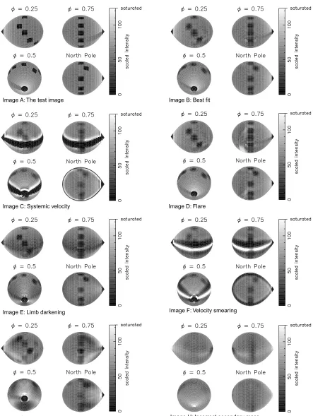
3.1 The test image

All our simulations are based on a single test image (Image A, Fig. 1). This image mimics the effect of irradiation of the secondary star by the compact primary, taking into account the distance to the companion and the incidence angle at the surface of the star. The intensity of the side of the star that is not irradiated is set to the intensity at the terminator. Also, shielding by (for example) an accretion stream is mimicked by a narrow band stretching along the equator from the inner Lagrangian (L1) point to the terminator and covering 3.6 per cent of the total surface area. The intensity of this band is equal to the intensity of the non-irradiated side of the secondary.

In addition, an array of 10 completely dark spots are distributed around the star. Four are located on the trailing hemisphere centred at latitudes of approximately1508, 1258, 08and2258, all with different longitudes. Another four are located on the leading hemisphere at latitudes of1508,1258, 08and2368, all with the same longitude. The two final spots are located at the north pole (1908) and the L1point. Each spot covers 0.7 per cent of the total surface area of the secondary, with the exception of the L1 spot which covers 1 per cent.

Finally, the geometry of the Roche lobe itself is given by the binary parameters M1¼1:0 M(, M2¼0:5 M( and an orbital

period of 2 h. Unless otherwise stated, the orbital inclination used was 608. In total, the image consists of 3008 elements which, with these binary parameters, gives a maximum radial velocity difference between any two neighbouring elements of 18.1 km s21.

3.2 Synthetic data sets and fits

Unless otherwise stated, a perfect synthetic trailed spectrum was computed assuming an instrumental resolution of 20 km s21_{and a} negligible intrinsic linewidth. The whole orbit was sampled over 50 evenly spaced phased bins, with a velocity bin width of 10 km s21

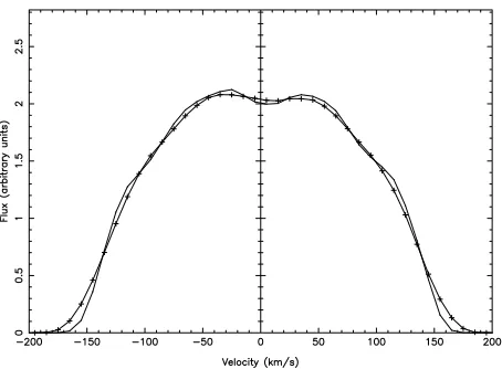
and a negligible exposure time. No contribution from an accretion disc or other part of the system was considered. A sample trailed spectrum is shown in Fig. 2 and the best fit to this data set is displayed in Image B, Fig. 1.

In each case the initial guess at the fit was one of uniform intensity distribution, and a uniform default map was used except in Section 3.14. Due to the nature of the tests, the fits could not proceed to the same finalx2on each occasion. Thus the optimal fit was determined by minimizing x2 until the spot features were resolved.

The reconstructions are plotted using a linear grey-scale. A value of 100 corresponds to the maximum intensity on the original test image (Image A, Fig. 1). Any intensity value,22 per cent greater than the maximum intensity of the test image is flagged as white. This is because some artefacts generate ‘hot’ elements with high intensities which would otherwise dominate the grey-scale plots.

We are now ready to explore the effects of systematic errors on the Roche tomography reconstructions. In each case a fake data set was generated that was either corrupted in some form or was fitted assuming an incorrect parameter.

3.3 Systemic velocityg

The systemic velocity is the radial velocity of the centre-of-mass of the binary system, and represents the mean shift of the line from its rest wavelength. In cases where the wrong value for the systemic velocity is assumed, the reconstruction process will have difficulty in fitting the line profiles. As a result, artefacts will be generated in order to allow the model to fit the profiles as well as possible. Due to the high quality of the synthetic data sets used, one might expect a small error in the systemic velocity to produce noticeable artefacts. Image C (Fig. 1) shows the effects of ignoring a systemic velocity of 15 km s21 present in the data. Although the spot features and, to some extent, the irradiated inner face of the secondary are still visible in the reconstruction, dark bands framed by bright stripes are formed around the equatorial regions.

These equatorial stripes can be explained as follows. When fitting the trailed spectrum the data appears to be ‘skewed’ to one side of the radial velocity axis, and therefore the model cannot possibly fit the edges of the line profiles. At the lower (or most negative) radial velocities expected by the model there are no data, the data that should have been present at these velocities having been shifted to a higher radial velocity. Thus the model attempts to

fit zero intensity to the regions of the star that contribute to the line profile at these points, resulting in a dark equatorial band.

At the other extreme, the higher (or most positive) radial velocities in the line profiles are shifted beyond the velocities expected by the model. Thus the intensities found at the highest radial velocities are far greater than expected by the model, and the opposite scenario emerges. The model now attempts to fit high intensities to the regions that contribute to the line profiles at these points. As only the equatorial regions ever contribute to the edges of the line profiles, a bright equatorial band results. The algorithm does not allow negative image values, which means it has greater freedom in setting the intensity (and hence the location) of the bright band. The bright band therefore borders the dark band, which lies on the equator.

3.4 Time variability

One of the key assumptions of our model is that features on the surface of the secondary do not vary during the course of an observation, e.g., a spot does not suddenly appear/disappear at a particular binary phase. Here we explore how a variation in the line flux from one region of the secondary may effect the reconstruction by simulating the presence of a flare. The flare is situated on the equator of the leading hemisphere (phase 0.75) and displaced slightly towards the back of the star. It is only present between phases 0.8 and 0.92 inclusive, has approximately 6 times the intensity of the surrounding non-irradiated region, and covers 0.7 per cent of the total surface area.

In the reconstruction (Image D, Fig. 1) a bright region can be seen at phase 0.75. This region is at roughly the same longitude, but at a much lower latitude than the actual position of the flare. This shift in latitude is easily explained: due to the orbital inclination, regions near the south pole are visible for shorter periods than the equatorial regions. By placing a bright region there, the fitting routine is trying to account for the limited phase coverage over which the flare is observed. However, in doing so the model must smear this feature in order to match the observed radial velocities of the flare. In addition, bright ‘ringing’ can be seen, which is due to the limited phase coverage over which the flare is observed; an

explanation of this effect will be given in more detail in Section 3.12.

3.5 Limb darkening

In Section 2 we mentioned that the line profile is scaled to take into account limb darkening. The fitting procedure cannot, without prior information, account for limb darkening. This is because limb darkening causes each element in the map to have a phase-dependent intensity variation. We must therefore supply the fitting procedure with an appropriate limb darkening relation. In this section we show the effects of assigning incorrect limb darkening strengths and laws.

First, data were generated assuming a linear limb darkening coefficient of 0.5. This was then fitted assuming no limb darkening (Image E, Fig. 1). The spot features are readily visible, although a dark equatorial band is formed. This band can be understood, because the model calculates much higher intensities at the edges of the profiles than are present in the fake data set. As described in Section 3.3, this results in dark equatorial bands in the reconstruction. In addition, the overall intensity level of the map is less than that of the test image due to the reduction in light caused by the limb darkening. Conversely, if one assumes too high a limb darkening coefficient, then the opposite occurs. The model calculates much lower intensities at the edges of the profiles and, in order to compensate the fitting routine, produces bright bands around the equator.

For our second test, we assumed an incorrect limb darkening law. Data generated using a linear limb darkening coefficient of 0.5 was then fitted assuming quadratic limb darkening coefficients of

a¼20:025,b¼0:635 and

IðmÞ ¼I1½12að12mÞ2bð12mÞ2Š;

wherem¼cosg,gis the angle between the line of sight and the emergent flux, and I1 is the monochromatic specific intensity at m¼1. The reconstruction showed a bright band around the equatorial regions where the fitting routine has had to compensate for the increased limb darkening predicted by the quadratic limb darkening law in this case.

3.6 Velocity smearing

Velocity smearing is the degradation in spectral resolution due to the combined effects of a finite exposure time and the orbital motion of the secondary star. Velocity smearing can be ignored if it is insignificant compared to the instrumental resolution. To obtain adequate signal-to-noise ratios, however, exposure times,texp, are usually selected which match the resulting velocity smearing to the instrumental resolution,vres, via the formula

texp,Pvres/2pKR; ð1Þ

whereP is the orbital period of the binary, andKRis the radial

velocity semi-amplitude of the secondary star. In cases where longer exposure times are unavoidable, significant velocity smearing will occur. It is possible to correct for the effects of velocity smearing in Roche tomography by calculating the line profiles at intermediate phases during an exposure, and averaging the results. This slows the iterations, however, so in this section we explore what happens if velocity smearing is neglected during the reconstruction process.

Image F (Fig. 1) shows what happens when an exposure time Figure 3. Solid line: line profile at phase 0, computed assuming zero

twice as long as that required by equation (1) is assumed when generating fake data and then ignored in the reconstruction process. Once again, the largest effects are seen in the equatorial regions. Fig. 3 shows why this occurs. The radial velocities of the edges of the smeared profile extend beyond the velocities expected when the exposure time is ignored. For the same reasons as discussed in Section 3.3, this results in bright and dark artefacts around the equator. Fig. 3 also shows how bumps in the line profile due to star-spots (e.g., the dip around 0 km s21) are smeared, resulting in a blurring of the star-spots in the reconstruction.

3.7 Intrinsic line profile width

We have so far assumed that the intrinsic line-profile width is negligible in comparison with the rotational broadening. This may not always be the case, and the width or shape of the intrinsic line profile may be important. Here we examine the effects of assuming an incorrect intrinsic line-profile width.

Data were produced assuming 20 km s21instrumental resolution as before, but with an intrinsic profile width of 45 km s21(FWHM). The reconstruction was carried out assuming no intrinsic line-profile width, and the result was very similar to Image F (Fig. 1). Once more, the edges of the lines cannot be fitted, and banding is hence seen around the equator. The reconstruction also shows that the spots are broadened. This is due to the algorithm attempting to match the width of the bumps in the line profile which, in the absence of intrinsic broadening, it can only do by increasing the size of the spots in the reconstruction.

3.8 Eclipse by an accretion disc

The highest inclination CVs may show signs of an eclipse of the secondary star by an accretion disc around phase 0.5. This can be accounted for during the reconstruction process either by removing the affected spectra (as commonly done in Doppler tomography during primary eclipse), or by including the eclipse in the algorithm. If neither of these steps is taken, artefacts will be introduced in the reconstructions, as described in this section.

A model including a cylindrical accretion disc of radius 0.5RL1

and height 0.1Rdiscwas created, and a synthetic trailed spectrum including the eclipse by the disc was generated assumingi¼808. Image G (Fig. 1) shows the reconstruction if the eclipse by the accretion disc is ignored. As one might expect, the artefacts generated by the eclipse are most apparent around the L1point. In particular, the southern regions (where light is blocked by the eclipse) appear dark, and there are alternating regions of bright and dark bands radiating from the L1 point. These are due to the attempts of the fitting algorithm to match the eclipse phases, resulting in a reduction of intensity on the inner hemisphere which is compensated for at other phases by the bright bands. Note that the spot features are well reconstructed, but exhibit the mirroring effect described in Section 3.11 due to the high inclination.

3.9 Masses

A knowledge of the binary masses is essential in order to define the geometry of the secondary star model. Very few accurate mass determinations are available for CVs, however, and although we can use Roche tomography to determine them (see Section 4), we still need to know how an error in the masses may effect the reconstructions.

Image H (Fig. 1) shows the effect of underestimating the

secondary mass by 0.1 M(. The effect of reducing the secondary’s

mass whilst keeping the period and inclination the same is to shift the model to higher radial velocities. Hence the spot features on the reconstruction appear shifted towards the L1point and lower radial velocities in order to compensate for this. In addition, as the radial velocities of the spot features in the original data set no longer correspond to a well-defined location on the secondary, the spots appear smeared over a larger area. At phases 0.25 and 0.75 the outer hemisphere of the model is shifted to higher radial velocities than present in the data set, and hence a dark band is formed near the rear of the star. At other phases the model cannot match the width of the line profiles due to the reduced radius of the star, and this results in a bright equatorial band.

3.10 Inclination

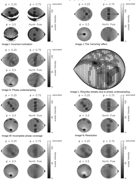
Up until now we have always assumed the correct orbital inclination (608) in each of our tests. In reality, however, we may not know the inclination accurately. Image I (Fig. 1) shows the effect of assuming an incorrect inclination of 558.

Once again, the most obvious artefacts appear at the equatorial regions. The lower orbital inclination shifts the model to lower radial velocities. As a consequence, the greatest mismatch between the observed and computed trailed spectra occur around phases 0.25 and 0.75. At the lowest radial velocities expected by the model there are no data, and a similar scenario occurs to that discussed in Section 3.3; dark bands are fitted around the equator on the inner hemisphere of the star to compensate for the lack of data at these velocities. Bright regions then appear around the dark band in order to fit the intensities seen at other phases. At higher radial velocities around phases 0.25 and 0.75, the observed intensity is far greater than predicted by the model, and the opposite occurs on the outer hemisphere of the star.

The spot features remain visible, but are systematically shifted towards the outer hemisphere of the star. This shifts them to regions of the star with higher radial velocities, which is necessary to counteract the shift of the model to lower radial velocities caused by assuming an incorrect inclination. The opposite occurs if too high a value for the orbital inclination is assumed; the dark bands become bright, and the spot features are systematically shifted towards the inner hemisphere and lower radial velocities.

3.11 The mirroring effect

The following sections describe artefacts that are not strictly due to systematic errors, but are a result of factors that are either within our control (e.g., instrumental resolution, phase sampling) or are inherent to the reconstruction process itself.

3.12 Phase sampling

Up until now, our simulations have been carried out over 50 evenly sampled phase bins covering a whole binary orbit. In practice, however, it may not always be possible to obtain this number of phases due to signal-to-noise requirements, or there may be gaps in the orbital coverage because of weather conditions. Here we model such scenarios.

First, we explore how undersampling in phase can affect the reconstruction. Image K (Fig. 1) was reconstructed from six evenly spaced phases (five independent) using zero exposure lengths,1and it is dominated by ring-like streaks. The effect is analogous to the streaks observed in Doppler tomography (Marsh & Horne 1988), and can be understood by considering that lines of constant radial velocity on the secondary star at a particular phase can be integrated along to construct a line profile. These lines of constant radial velocity are ring-like in shape and, if there are only a few phases, or if the profile is particularly bright at a certain phase (as in the case of a flare; Section 3.4), the streaks will not destructively interfere, leaving ring-like artefacts on the Roche tomogram. To demonstrate this effect, we produced maps where those elements with the same radial velocity as the spot features were represented as a grey-scale, whilst all other elements were left blank. This was done for each of the six phases in the data set, and the resulting images were then superimposed on top of one another so that regions where streaks overlap are shown darker (Image L, Fig. 1). It can be seen that the features in this image closely resemble the artefacts in Image K (Fig. 1).

Image M (Fig. 1) shows the effect of incomplete phase coverage, with phases between 0.4 and 0.6 missing (which may occur if certain phases are discarded due to, for example, an eclipse by the disc; see Section 3.8). There is no problem recovering the features around the L1 point where the majority of the information is missing. Although the other spot features are also readily recovered, they appear elongated or streaked due to the same process as that described in the above paragraph.

3.13 Instrumental resolution

The spectral resolution of the data governs the size of the features that can be imaged, as shown by the blurred spots in Image N (Fig. 1) where we have reconstructed the test image using data of lower resolution (60 km s21) than before. The number of surface elements in the model should be chosen to match the spectral resolution. If the model has too few elements, the separation between adjacent elements in velocity space (particularly around phases 0.25 and 0.75) is greater than the resolution of the data. This means that there will be parts of the line profile to which no surface elements in the model contribute (at a particular phase), and no acceptable fit will be found. If, on the other hand, too many elements in the model are used, there will be no problem in fitting the data, but it will slow the reconstruction process.

3.14 Default maps

In the reconstruction process the final map is the one of maximum entropy (relative to an assumed default map) which is consistent

with the data. If the data are good then the final map is constrained by the data, and will not be strongly influenced by the default. In this case the choice of default makes little difference to the final map. If the data are noisy, however, the data constraints will be weak, and the map will be strongly influenced by the default. The default can therefore be regarded as containing prior information about the map, and regions of the map that are not constrained by the data will converge to the default value.

To investigate the effect of different default maps on the reconstruction, it is necessary to degrade the quality of the test data set. We therefore generated data over 15 phase bins with a resolution of only 60 km s21and a signal-to-noise ratio of only 50. The data set was then fitted using a uniform default map and a Gaussian-blurr default map. The former was created by setting every element in the default to the average value of the map, and hence constrains large-scale surface structure. The latter was created by smoothing the map using a Gaussian-blurring function, and hence constrains small-scale surface structure.

Image O (Fig. 1) shows the reconstruction using the uniform default map and, as expected, it can be seen that the spots are more blurred than in the reconstruction using the Gaussian-blurr default map (Image P, Fig. 1). Features below 2608 latitude are never visible, and hence in the fitting routine they are assigned a value determined by the default map. In the case of the uniform default map, this is the average element value of the map. In the case of the Gaussian-blurr default map, however, the value assigned depends upon the intensity values of the neighbouring elements and, for elements that are not visible, this is close to zero intensity. This explains why the reconstruction using the Gaussian-blurr default has a dark southern limb and, to compensate for this, a bright region above the L1point. Hence, although the use of a Gaussian-blurr default is more likely to resolve small features, it is important to be aware of the effects that visibility may have on the final outcome.

4 D E T E R M I N I N G P H Y S I C A L PA R A M E T E R S : T H E E N T R O P Y L A N D S C A P E

If the centre-of-light and centre-of-mass of the secondary are not coincident, the star’s radial-velocity curve will be distorted in some way from the pure sine wave which represents the motion of its centre-of-mass. The observed radial velocity curves of CV secondaries suffer from this distortion, due to both geometrical effects caused by the Roche-lobe shape and non-uniformities in the surface distribution of the line strength due to, for example, irradiation. If these factors are ignored, they will lead to systematic errors in the determination of the binary star masses.

By modelling the shape and mapping the surface intensity distribution of the secondary star, Roche tomography can provide constraints on the CV masses. This is because, as discussed in Section 3.9, incorrect values ofM1andM2will introduce artefacts in the reconstructions which will lower the entropy of the final solution. The correct values of the component masses are therefore those that produce the map of highest entropy.

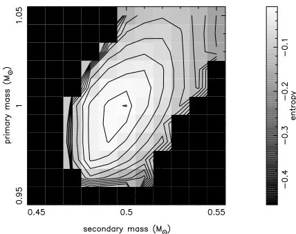
This is demonstrated in Fig. 4, which displays the ‘entropy landscape’ of the test data shown in Fig. 2. Each square in the entropy landscape corresponds to the maximum entropy obtained in a reconstruction assuming a particular pair of component mass values, a uniform default map and iterating to the samex2value on each occasion. The reconstruction with the highest entropy was obtained for component masses of M1¼1:0 M( and

M2¼0:5 M(, which are identical to the masses used to construct

1_{Although such a scenario would probably only occur if long exposure}

the test data. This shows the entropy-landscape method to be an extremely effective method of determining accurate component masses which accounts for both geometrical distortion and complicated intensity distributions on the secondary star. Note that the correct inclination was used for every reconstruction in Fig. 4, but in practice the inclination may not be accurately known. A similar method to the entropy landscape can then be used to determine the inclination or, in cases where the secondary eclipses the white dwarf, the inclination can be varied for each combination of component masses in order to remain consistent with the observed eclipse width.

Fig. 4 also shows a ridge of high entropy running along a line of (almost) constantq. Component masses lying along this diagonal are therefore more difficult to distinguish than component masses lying perpendicular to it. The gradient of the diagonal can be derived by considering that the best fit is obtained when the centre of the model line profile matches the centre of the observed profile. The centre of the line profile is governed by the radial velocity of the secondary, which relates directly to the distance of the centre-of-mass of the secondary from the centre-centre-of-mass of the binary,a2. Thus only those combinations ofM1andM2that maintain constant

a2can provide satisfactory fits to the data. Using Kepler’s law and assuming a constant period anda2, we can show that the ridges in the entropy landscape correspond to component masses which obey the relation

M1

ðM11M2Þ2=3

¼ constant: ð2Þ

This simple argument becomes complicated in the case of irradiation. Rutten & Dhillon (1994) found that the ridge of high entropy was shifted towards slightly higher values of M2. Their explanation for this was that the intensity distribution was strongly peaked towards the L1point, causing a large difference with the uniform default map. This difference was reduced by increasing

M2, allowing the bright region to shift away from the L1point and to spread over more elements, reducing the deviation between the map and the default whilst still fitting the trailed spectrum to within its uncertainties. Despite this, the mass determination was still correct to within,2 per cent.

Another feature of note in the entropy landscape in Fig. 4 is that, as the primary mass increases, there is a larger range of secondary masses that can be fitted satisfactorily. This can be explained by generalizing equation (2) to

q11/M11=2;

which shows that as the primary mass increases, the mass ratio,

q¼M2/ M1, must also increase in order to holda2constant. It can be shown that the secondary star radius is related to q and a2 according to

R2/ a2/q1=3ð11qÞ2=3;

which shows that the radius of the secondary star must increase ifq

increases. This in turn means that the model linewidth is greater than the observed linewidth, and this overlap allows a greater range of secondary star geometries for which a satisfactory fit can be obtained. In contrast, at low primary masses the allowed value ofq

is decreased, resulting in a low secondary star radius and hence a small model linewidth. At the lowest primary masses in Fig. 4, the model linewidths become too narrow to fit the observed profile to the desiredx2, no matter what intensity pattern is mapped on to the

secondary star’s surface, explaining the abrupt end of the high-entropy ridge on the lower left-hand portion of Fig. 4.

It is important to note that the maximum-entropy algorithm we use requires that all input data are positive. As a result, it is necessary to invert absorption-line profiles and, in the case of low signal-to-noise data, add a positive constant in order to ensure that there are no negative values in the continuum-subtracted spectra. If this positive constant is not added, and any negative points are either set to zero or ignored during the reconstruction, the fit will be positively biased in the line wings, resulting in a broader computed profile and hence larger stellar masses in the entropy landscape. It is a simple matter to account for this positive constant during the reconstruction process by employing a virtual image element which contributes a single value to all data points, effectively cancelling out the constant. This virtual image element can also be used to correct for small errors in the continuum subtraction, which might otherwise systematically affect the masses derived from the entropy landscape.

5 S TAT I S T I C A L E R R O R S

Although it is possible to propagate the statistical errors on the data points through the iterative process in order to calculate the statistical errors on each element in the map, the resulting error bars are unreliable due to the fact that noise in Roche tomograms is correlated. This correlation arises from the projection of bumps in the profile along arcs of constant radial velocity on the secondary star and from the effects of blurring by the default map. Doppler imaging of single stars has largely relied on consistency tests, such as comparing image reconstructions using either subsets of observations (e.g. Barnes et al. 1998) or different spectral lines (e.g. Strassmeier & Bartus 2000), in order to address this issue. So far, the only attempt at a formal statistical error analysis in Doppler imaging has been undertaken using the Occamian approach (Berdyugina 1998).

are therefore not as strongly constrained as Doppler images of single stars by the input data. This makes the determination of statistical errors of prime importance in Roche tomography, because only then can one test whether a surface feature is real or just a spurious artefact due to noise.

We have addressed the problem of statistical error determination in Roche tomography using a Monte Carlo approach. Monte Carlo techniques rely on the construction of a large (typically hundreds, in the case of Roche tomography) sample of synthesized data sets which have been effectively drawn from the same parent population as the original data set, i.e., as if the observations have been repeated many hundreds of times. This large sample of synthesized data sets is then used to create a large sample of Roche tomograms, resulting in a probability distribution for each element in the map. The main difficulty with this technique, aside from the demands on computer time, lies in the construction of the sample of synthesized data sets. One approach (used by Rutten et al. 1994 in spectral eclipse mapping) is to ‘jiggle’ each data point about its observed value, by an amount given by its error bar multiplied by a number output by a Gaussian random-number generator with zero mean and unit variance. This process adds noise to the data, however, which means that the synthesized data sets are not being drawn from the same parent population as the observed data set – noise is being added to a data set which has already had noise added to it during the measurement process. In practice, this means that fitting the sample data sets to the same level ofx2

as the original data set is either impossible (i.e., the iteration does not converge) or results in maps dominated by noise, which grossly overestimates the true error on each element. We have verified that

this is the case using simulations similar to those described in Section 5.1.

Instead, we have opted for the bootstrapping technique of Efron (1979); see Efron & Tibshirani (1993) for a general introduction to the method. We implemented the bootstrap as follows. From our observed trailed spectrum containing ndata points we form our synthesized trailed spectrum by selecting, at random and with replacement, n data values and placing these at their original positions in the new synthesized trailed spectrum. For points that are not selected we set the associated error bar to infinity and thereby effectively omit these points from the fit. For points that have been selected once or more than once (typically 37 per cent of the points) we divide their error bars by the square root of the number of times they were picked. The advantage of bootstrap re-sampling over jiggling is that the data are not made noisier by the process as only the errors bars on the data points are manipulated (i.e., the data values remain unchanged). In so doing, the amount of noise present in the data is conserved, and it is therefore possible to fit the synthesized trailed spectra to the same level ofx2as the observed data, giving a much more reliable estimate of the statistical errors in the maps.

5.1 Testing the bootstrap

In order to assess the viability of the bootstrap technique, we ran a simple test. A model with parameters M1¼1:0 M(,

M2¼0:5 M(, i¼608 and P¼2:78 h was created of uniform

intensity distribution, with the exception of a single spot covering 0.8 per cent of the total surface area on the trailing hemisphere (see Fig. 5). From this model a synthetic trailed spectrum was generated with 30 evenly spaced phase bins and 60 km s21 instrumental resolution. Each data point in the spectrum was then ‘jiggled’ by 10 per cent of the original data value in order to simulate noise. A close fit to this data set was then carried out using the correct parameters.

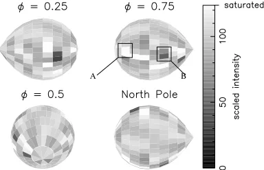
As can be seen, the reconstruction (Fig. 6) shows many spurious artefacts due to noise. Fitting to a higherx2, whilst removing some of the lower level noise artefacts, does not remove the spurious spot features marked A and B in Fig. 6. The triangular symbols in Fig. 7 show the intensities in each vertical slice through A, B and the real spot. It can be seen that, from this information alone, it is impossible to deduce which spot features are real.

The curves in Fig. 7 show the confidence intervals found after reconstructing 200 bootstrap samples of the image. As the distribution of element intensities found is often non-normal and not centred on the intensity found in the original fit (see Fig. 8), it is incorrect to calculate a summary error statistic like the standard deviation. Instead, we take the mode of the distribution to represent the ‘most probable’ value, and define the 95 per cent confidence interval (for example) as the region which encloses 95 per cent of the bootstrap values above and below the mode. It can be seen that the confidence intervals in Fig. 7 widen significantly around the noise features A and B, and encompass the true intensity level (indicated by the horizontal line). The confidence intervals around the real spot feature, however, do not exhibit such a widening, and clearly do not encompass the true intensity level of the non-spotted regions. This test therefore confirms that the bootstrapping method works; it has correctly identified the real spot feature and correctly identified features A and B as artefacts due to noise. In a similar test, statistical errors determined by the method of ‘jiggling’ failed to distinguish between the real spot and features A and B.

There are two additional features of note in Fig. 7. First, it can be Figure 5.The test image used to construct the noisy data set described in

Section 5.1

Figure 6.The Roche tomography reconstruction of the test image in Fig. 5 using noisy data. Although the spot can be seen at phase 0.25, many spurious artefacts due to noise are also present, including features A and B.

seen that in regions where the data do not constrain the intensity distribution (such as the southern hemisphere, which is never visible), the reconstruction always converges to the default map value, which is why the confidence intervals converge around ‘SP’ in Fig. 7. Second, the slices through features A and B demonstrate how noise is correlated in the Roche tomography reconstruction process, because elements surrounding the peak intensity are all shifted in the same direction as the peak itself.

6 C O N C L U S I O N S

We have shown that any feature on a Roche tomogram must be subjected to two tests before its reality can be confirmed. The first test is to determine whether the feature is statistically significant, and is performed using a Monte Carlo technique. The conventional method, where hypothetical data sets are constructed by ‘jiggling’ the data in accordance with their error bars, was found to add noise and hence grossly overestimate the errors in the reconstruction. The solution to this problem was found by using a bootstrap Figure 7.Triangles: intensity values along vertical slices through A (top), B (middle) and the real spot (bottom) in Fig. 6. Curves: confidence intervals along vertical slices through A (top), B (middle) and the real spot (bottom) in Fig. 6. LH, NP, TH and SP at the top of the figure represent the positions of elements at the leading hemisphere, north pole, trailing hemisphere and south pole, respectively.

re-sampling algorithm and, through the use of simulations, we have shown this technique to correctly distinguish between real features and artefacts due to noise. The second test is to compare the feature with the appearance of known artefacts of the technique. In general, we find that systematic errors result in only three major artefacts in the Roche tomograms: ring-like streaks, equatorial banding and blurring. The effects of these artefacts can be minimized, however, by fine-tuning the input parameters. A fine example of this is given by the entropy landscape technique, which also provides accurate component masses. If a surface feature survives both of the above tests unscathed, it can be assumed to be real.

A C K N O W L E D G M E N T S

We thank Chris Careless, Antonio Claret, Tom Marsh, Rene´ Rutten and Tariq Shahbaz for their help in the work which led to this paper. CAW is supported by a PPARC studentship. The authors acknowledge the data analysis facilities at Sheffield provided by the Starlink Project, which is run by CCLRC on behalf of PPARC.

R E F E R E N C E S

Barnes J. R., Collier Cameron A., Unruh Y. C., Donati J. F., Hussain G. A. J., 1998, MNRAS, 299, 904

Berdyugina S. V., 1998, A&A, 338, 97

Bruls J. H. M. J., Solanki S. K., Schussler M., 1998, A&A, 336, 231 Cameron A. C., Foing B. H., 1997, Observatory, 117, 218

Dhillon V. S., Watson C. A., 2001, in Boffin H., Steeghs D., eds,

Proceedings of the International Workshop on Astro-tomography, Brussels, July 2000. Springer-Verlag Lecture Notes in Physics, in press Efron B., 1979, Annals of Statistics, 7, 1

Efron B., Tibshirani R. J., 1993, An Introduction to the Bootstrap. Chapman & Hall, New York

Hatzes A. P., Vogt S. S., Ramseyer T. F., Misch A., 1996, ApJ, 469, 808 Maceroni C., Vilhu O., van’t Veer F., Van Hamme W., 1994, A&A, 288, 529 Marsh T. R., Horne K., 1988, MNRAS, 235, 269

Ramseyer T. F., Hatzes A. P., Jablonski F., 1995, AJ, 110, 1364 Rutten R. G. M., 1987, A&A, 177, 131

Rutten R. G. M., Dhillon V. S., 1994, A&A, 288, 773

Rutten R. G. M., Dhillon V. S., 1996, in Evans A., Wood J. H., eds, Cataclysmic Variables and Related Objects. Kluwer Academic Publishers, Dordrecht, p. 21

Rutten R. G. M., Dhillon V. S., Horne K., Kuulkers E., 1994, A&A, 283, 441

Skilling J., Bryan R. K., 1984, MNRAS, 211, 111 Smith D. A., Dhillon V. S., 1998, MNRAS, 301, 767

Smith R. C., 1995, in Buckley D. A. H., Warner B., eds, ASP Conf. Ser. Vol. 85, Cape Workshop on Magnetic CVs. Astron. Soc. Pac., San Francisco, p. 417

Strassmeier K. G., Bartus J., 2000, A&A, 354, 537 Unruh Y. C., Collier Cameron A., 1995, MNRAS, 273, 1 Unruh Y. C., Collier Cameron A., 1997, MNRAS, 290, L37 Vogt S. S., Penrod G. D., 1983, PASP, 95, 565

Warner B., 1995, Cataclysmic Variable Stars. Cambridge Univ. Press, Cambridge