Index Design and the
Optimizers
Relational Database
Index Design and the
Optimizers
DB2, Oracle, SQL Server, et al.
Tapio Lahdenm¨aki
Michael Leach
Published by John Wiley & Sons, Inc., Hoboken, New Jersey. Published simultaneously in Canada.
No part of this publication may be reproduced, stored in a retrieval system, or transmitted in any form or by any means, electronic, mechanical, photocopying, recording, scanning, or otherwise, except as permitted under Section 107 or 108 of the 1976 United States Copyright Act, without either the prior written permission of the Publisher, or authorization through payment of the appropriate per-copy fee to the Copyright Clearance Center, Inc., 222 Rosewood Drive, Danvers,
the Publisher for permission should be addressed to the Permissions Department, John Wiley & Sons, Inc., 111 River Street, Hoboken, NJ 07030, (201) 748-6011, fax (201) 748-6008, or online at http://www.wiley.com/go/permission.
Limit of Liability/Disclaimer of Warranty: While the publisher and author have used their best efforts in preparing this book, they make no representations or warranties with respect to the accuracy or completeness of the contents of this book and specifically disclaim any implied warranties of merchantability or fitness for a particular purpose. No warranty may be created or extended by sales representatives or written sales materials. The advice and strategies contained herein may not be suitable for your situation. You should consult with a professional where appropriate. Neither the publisher nor author shall be liable for any loss of profit or any other commercial damages, including but not limited to special, incidental, consequential, or other damages.
For general information on our other products and services please contact our Customer Care Department within the U.S. at 877-762-2974, outside the U.S. at 317-572-3993 or
fax 317-572-4002.
Wiley also publishes its books in a variety of electronic formats. Some content that appears in print, however, may not be available in electronic format. For more information about wiley
Library of Congress Cataloging-in-Publication Data: Lahdenm¨aki, Tapio.
Relational database index design and the optimizers : DB2, Oracle, SQL server et al / Lahdenm¨aki and Leach.
p. cm.
Includes bibliographical references and indexes. ISBN-13 978-0-471-71999-1
ISBN-10 0-471-71999-4 (cloth)
1. Relational databases. I. Leach, Mike, 1942- II. Title. QA76.9.D3L335 2005
005.7565—dc22
2004021914
Printed in the United States of America.
10 9 8 7 6 5 4 3 2 1
MA 01923, 978-750-8400, fax 978-750-4470, or on the web at www.copyright.com. Requests to
Preface xv
1 Introduction 1
Another Book About SQL Performance! 1 Inadequate Indexing 3
Myths and Misconceptions 4
Myth 1: No More Than Five Index Levels 5 Myth 2: No More Than Six Indexes per Table 6 Myth 3: Volatile Columns Should Not Be Indexed 6 Example 7
Disk Drive Utilization 7 Systematic Index Design 8
2 Table and Index Organization 11
Introduction 11
Index and Table Pages 12 Index Rows 12
Index Structure 13 Table Rows 13
Buffer Pools and Disk I/Os 13
Reads from the DBMS Buffer Pool 14 Random I/O from Disk Drives 14 Reads from the Disk Server Cache 15 Sequential Reads from Disk Drives 16 Assisted Random Reads 16
Assisted Sequential Reads 19
Synchronous and Asynchronous I/Os 19 Hardware Specifics 20
DBMS Specifics 21 Pages 21
Table Clustering 22 Index Rows 23
Table Rows 23 Index-Only Tables 23 Page Adjacency 24
Alternatives to B-tree Indexes 25 Many Meanings of Cluster 26
3 SQL Processing 29
Introduction 29 Predicates 30
Optimizers and Access Paths 30
Index Slices and Matching Columns 31 Index Screening and Screening Columns 32 Access Path Terminology 33
Monitoring the Optimizer 34 Helping the Optimizer (Statistics) 34
Helping the Optimizer (Number of FETCH Calls) 35 When the Access Path Is Chosen 36
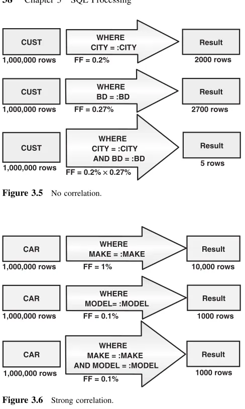
Filter Factors 37
Filter Factors for Compound Predicates 37 Impact of Filter Factors on Index Design 39 Materializing the Result Rows 42
Cursor Review 42
Alternative 1: FETCH Call Materializes One Result Row 43 Alternative 2: Early Materialization 44
What Every Database Designer Should Remember 44 Exercises 44
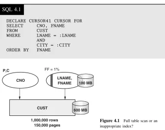
4 Deriving the Ideal Index for a SELECT 47
Introduction 47
Basic Assumptions for Disk and CPU Times 48 Inadequate Index 48
Three-Star Index—The Ideal Index for a SELECT 49 How the Stars Are Assigned 50
Range Predicates and a Three-Star Index 52
Algorithm to Derive the Best Index for a SELECT 54 Candidate A 54
Candidate B 55
Ideal Index for Every SELECT? 56 Totally Superfluous Indexes 57 Practically Superfluous Indexes 57 Possibly Superfluous Indexes 58 Cost of an Additional Index 58
Response Time 58 Drive Load 59 Disk Space 61 Recommendation 62 Exercises 62
5 Proactive Index Design 63
Detection of Inadequate Indexing 63 Basic Question (BQ) 63
Warning 64
Quick Upper-Bound Estimate (QUBE) 65 Service Time 65
Queuing Time 66
Essential Concept: Touch 67 Counting Touches 69 FETCH Processing 70
QUBE Examples for the Main Access Types 71
Cheapest Adequate Index or Best Possible Index: Example 1 75 Basic Question for the Transaction 78
Quick Upper-Bound Estimate for the Transaction 78 Cheapest Adequate Index or Best Possible Index 79 Best Index for the Transaction 79
Semifat Index (Maximum Index Screening) 80 Fat Index (Index Only) 80
Cheapest Adequate Index or Best Possible Index: Example 2 82 Basic Question and QUBE for the Range Transaction 82 Best Index for the Transaction 83
Semifat Index (Maximum Index Screening) 84 Fat Index (Index Only) 85
6 Factors Affecting the Index Design Process 87
I/O Time Estimate Verification 87 Multiple Thin Index Slices 88
Simple Is Beautiful (and Safe) 90 Difficult Predicates 91
LIKE Predicate 91
OR Operator and Boolean Predicates 92 IN Predicate 93
Filter Factor Pitfall 94
Filter Factor Pitfall Example 96 Best Index for the Transaction 99
Semifat Index (Maximum Index Screening) 100 Fat Index (Index Only) 101
Summary 101 Exercises 102
7 Reactive Index Design 105
Introduction 105
EXPLAIN Describes the Selected Access Paths 106 Full Table Scan or Full Index Scan 106
Sorting Result Rows 106 Cost Estimate 107
DBMS-Specific EXPLAIN Options and Restrictions 108 Monitoring Reveals the Reality 108
Evolution of Performance Monitors 109 LRT-Level Exception Monitoring 111
Averages per Program Are Not Sufficient 111 Exception Report Example: One Line per Spike 111 Culprits and Victims 112
Promising and Unpromising Culprits 114 Promising Culprits 114
Tuning Potential 116 Unpromising Culprits 120 Victims 121
Call-Level Exception Monitoring 123 Oracle Example 126
SQL Server Example 129 Conclusion 131
DBMS-Specific Monitoring Issues 131 Spike Report 132
Exercises 133
8 Indexing for Table Joins 135
Introduction 135 Two Simple Joins 136
Example 8.1: Customer Outer Table 137 Example 8.2: Invoice Outer Table 138
Impact of Table Access Order on Index Design 139 Case Study 140
Current Indexes 143 Ideal Indexes 149
Ideal Indexes with One Screen per Transaction Materialized 153 Ideal Indexes with One Screen per Transaction Materialized and
FF Pitfall 157
Basic Join Question (BJQ) 158 Conclusion: Nested-Loop Join 160 Predicting the Table Access Order 161 Merge Scan Joins and Hash Joins 163
Merge Scan Join 163
Example 8.3: Merge Scan Join 163 Hash Joins 165
Program C: MS/HJ Considered by the Optimizer (Current Indexes) 166
Ideal Indexes 167
Nested-Loop Joins Versus MS/HJ and Ideal Indexes 170 Nested-Loop Joins Versus MS/HJ 170
Ideal Indexes for Joins 171 Joining More Than Two Tables 171 Why Joins Often Perform Poorly 174
Fuzzy Indexing 174
Designing Indexes for Subqueries 175 Designing Indexes for Unions 176 Table Design Considerations 176
Redundant Data 176
Unconscious Table Design 180 Exercises 183
9 Star Join Considerations 185
Introduction 185
Indexes on Dimension Tables 187
Huge Impact of the Table Access Order 188 Indexes on Fact Tables 190
Summary Tables 192
10 Multiple Index Access 195
Introduction 195 Index ANDing 195
Index ANDing with Query Tables 197 Multiple Index Access and Fact Tables 198 Multiple Index Access with Bitmap Indexes 198 Index ORing 199
Index Join 200 Exercises 201
11 Indexes and Reorganization 203
Physical Structure of a B-Tree Index 203 How the DBMS Finds an Index Row 204 What Happens When a Row Is Inserted? 205 Are Leaf Page Splits Serious? 206
When Should an Index Be Reorganized? 208 Insert Patterns 208
Volatile Index Columns 216 Long Index Rows 218
Example: Order-Sensitive Batch Job 219
Table Disorganization (with a Clustering Index) 222
Table Rows Stored in Leaf Pages 223 SQL Server 223
Oracle 224
Cost of Index Reorganization 225 Split Monitoring 226
Summary 227
12 DBMS-Specific Indexing Restrictions 231
Introduction 231
Number of Index Columns 231
Total Length of the Index Columns 232 Variable-Length Columns 232
Number of Indexes per Table 232 Maximum Index Size 232 Index Locking 232
Index Row Suppression 233
DBMS Index Creation Examples 234
13 DBMS-Specific Indexing Options 237
Introduction 237
Index Row Suppression 237
Additional Index Columns After the Index Key 238 Constraints to Enforce Uniqueness 240
DBMS Able to Read an Index in Both Directions 240 Index Key Truncation 241
Function-Based Indexes 241 Index Skip Scan 242 Block Indexes 243
Data-Partitioned Secondary Indexes 243 Exercises 244
14 Optimizers Are Not Perfect 245
Introduction 245
Optimizers Do Not Always See the Best Alternative 246 Matching and Screening Problems 246
Non-BT 247
Unnecessary Sort 250
Optimizers’ Cost Estimates May Be Very Wrong 252 Range Predicates with Host Variables 252
Skewed Distribution 253 Correlated Columns 255
Cautionary Tale of Partial Index Keys 256 Cost Estimate Formulas 259
Estimating I/O Time 259 Estimating CPU Time 261
Helping the Optimizer with Estimate-Related Problems 261 Do Optimizer Problems Affect Index Design? 265
Exercises 265
15 Additional Estimation Considerations 267
Assumptions Behind the QUBE Formula 267 Nonleaf Index Pages in Memory 268
Example 268
Impact of the Disk Server Read Cache 269 Buffer Subpools 270
Long Rows 272
Slow Sequential Read 272
When the Actual Response Time Can Be Much Shorter Than the
QUBE 272
Leaf Pages and Table Pages Remain in the Buffer Pool 273 Identifying These Cheap Random Touches 275
Assisted Random Reads 275 Assisted Sequential Reads 278 Estimating CPU Time (CQUBE) 278
CPU Time per Sequential Touch 278 CPU Time per Random Touch 279 CPU Time per FETCH Call 281 CPU Time per Sorted Row 282 CPU Estimation Examples 282
Fat Index or Ideal Index 283
Nested-Loop Join (and Denormalization) or MS/HJ 283 Merge Scan and Hash Join Comparison 286
16 Organizing the Index Design Process 289
Introduction 289
Computer-Assisted Index Design 290 Nine Steps Toward Excellent Indexes 292 References 295
Glossary 297
Index Design Approach 297 General 299
Relational databases have been around now for more than 20 years. In their early days, performance problems were widespread due to limited hardware resources and immature optimizers, and so performance was a priority consid-eration. The situation is very different nowadays; hardware and software have advanced beyond all recognition. It’s hardly surprising that performance is now assumed to be able to take care of itself! But the reality is that despite the huge growth in resources, even greater growth has been seen in the amount of information that is now available and what needs to be done with this infor-mation. Additionally, one crucial aspect of the hardware has not kept pace with the times: Disks have certainly become larger and incredibly cheap, but they are still relatively slow with regards to their ability to directly access data. Conse-quently many of the old problems haven’t actually gone away—they have just changed their appearance. Some of these problems can have enormous implica-tions—stories abound of “simple” queries that might have been expected to take a fraction of a second appear to be quite happy to take several minutes or even longer; this despite all the books that tell us how to code queries properly and how to organize the tables and what rules to follow to put the right columns into the indexes. So it is abundantly clear that there is a need for a book that goes beyond the usual boundaries and really starts to think about why so many people are still having so many problems today.
The second objective of this book is to show how we can use this knowledge to quantify the work being performed in terms of CPU and elapsed time. Only in this way can we truly judge the success of our index and table design; we need to use actual figures to show what the optimizer would think, how long the scans would take, and what modifications would be required to provide satisfactory performance. But most importantly, we have to be able to do this quickly and easily; this in turn means that it is vital to focus on the few really major issues, not on the relatively unimportant detail under which many people drown. This is key—to focus on a very few, crucially important areas—and to be able to say how long it would take or how much it would cost.
We have also one further advantage to offer, which again arises as a result of focusing on what really matters. For those who may be working with more than one relational product (even from the same vendor), instead of reading and digesting multiple sets of widely varying rules and recommendations, we are using a single common approach which is applicable to all relational products. All “genuine” relational systems have an optimizer that has the same job to do; they all have to make decisions and then scan indexes and tables. They all do these things in a startlingly similar way (although they have their own way of describing them). There are, of course, some differences between them, but we can handle this with little difficulty.
The audience for which this book is intended, is quite literally, anyone who feels it is to his or her benefit to know something about SQL performance or about how to design tables and indexes effectively, as well as those having a direct responsibility for designing indexes, anyone coding SQL statements as queries or as part of application programs, and those who are responsible for maintaining the relational data and the relational environment. All will benefit to a varying degree if they feel some responsibility for the performance effects of what they are doing.
Finally, a word regarding the background that would be appropriate to the readers of this book. A knowledge of SQL, the relational language, is assumed. A general understanding of computer systems will probably already be in place if one is even considering a book such as this. Other than that, perhaps the most important quality that would help the reader would be a natural curiosity and interest in how things work—and a desire to want to do things better. At the other extreme, there are also two categories of the large number of peo-ple with many years of experience in relational systems who might feel they would benefit; first those who have managed pretty well over the years with the detailed rule books and would like to relax a little more by understanding why these rules apply; second, those who have already been using the tech-niques described in this book for many years but who have not appreciated the implications that have been brought into play by the introduction of the new world hardware.
we are greatly indebted to numerous friends and colleagues who have assisted in so many ways and provided so much encouragement. In particular we would like to thank Matti St˚ahl for his detailed input and critical but extremely help-ful advice throughout the development of the book; Lennart Hen¨ang, Ari Hovi, Marja K¨armeniemi, Timo Raitalaakso for their invaluable assistance and reviews, and Akira Shibamiya for his original work on relational performance formulae. In addition we are indebted to scores of students and dozens of database consultants for providing an insight into their real live problems and solutions. Finally, a very special thanks go to Meta and Lyn without whose encouragement and support this book would never have been completed; Meta also brilliantly encapsulated the heart of the book in her special design for the bookcover. Solutions to the end-of-chapter exercises and other materials relating to this text can be found at this ftp address: ftp://ftp.wiley.com/public/sci tech med/relational database/.
TAPIOLAHDENM ¨AKI MICHAELLEACH Smlednik, Slovenia
Chapter
1
Introduction
ž To understand how SQL optimizers decide what table and index scans should be performed to process SQL statements as efficiently as possible
ž To be able to quantify the work being done during these scans to enable satisfactory index design
ž Type and background of audience for whom the book is written
ž Initial thoughts on the major reasons for inadequate indexing
ž Systematic index design.
ANOTHER BOOK ABOUT SQL PERFORMANCE!
Relational databases have been around now for over 20 years, and that’s precisely how long performance problems have been around too—and yet here isanother book on the subject. It’s true that this book focuses on the index design aspects of performance; however, some of the other books consider this area to a greater or lesser extent. But then a lot of these books have been around for over 20 years, and the problems still keep on coming. So perhaps there is a need for a book that goes beyond the usual boundaries and starts to think about why so many people are still having so many problems.
It’s certainly true that the world of relational database systems is a very complex one—it has to be if one reflects on what really has to be done to satisfy SQL statements. The irony is that the SQL is so beautifully simple to write; the concept of tables and rows and columns is so easy to understand. Yet we could be searching for huge amounts of information from vast sources of data held all over the world—and we don’t even need to know where it is or how it can be found. Neither do we have to worry about how long it’s going to take or how much it’s going to cost. It all seems like magic. Maybe that’s part of the problem—it’s too easy; but then of course, itshould be so easy.
We still recognize that problems will arise—and huge problems at that. Stories abound of “simple” queries that might have been expected to take a fraction of a second appear to be quite happy to take several minutes or even longer. But then, we have all these books, and they tell us how to code the query
Relational Database Index Design and the Optimizers, by Tapio Lahdenm¨aki and Michael Leach Copyright2005 John Wiley & Sons, Inc.
properly and how to organize the table and what rules to follow to put the right columns into the index—and often it works. But we still seem to continue to have performance problems, despite the fact that many of these books are really very good, and their authors really know what they are talking about.
Of particular interest to us in this book is the part of the relational system (called the SQL optimizer) thatdecides how to find all the information required in the most efficient way it can.In an ideal world, we wouldn’t even need to know it exists, and indeed most people are quite happy to leave it that way! Having made this decision, the optimizer directs scans of indexes and tables to find our data. In order to understand what’s going through the optimizer’s mind, we will also need to appreciate what is involved in these scans.
So what we want to do in this book is first to try to put ourselves in the optimizer’s place; how it decides what table and index scans should be performed to process SQL statements as efficiently as possible. Perhaps if we understandwhy it might have problems, we could do things differently; not by simply following a myriad of incredibly complex rules that, even if we can understand them might or might not apply, but by understanding what it is trying to do.
A major concern that one might reasonably be expected to have on hearing this is that it would appear to be too complex or even out of the question. But it is quite surprising how little we really need to understand; what there is, though, is incredibly important.
Likewise, perhaps the first, and arguably themost important, difference this book has from other books in its field is that we willnot be providing a massive list of rules and syntax to use for coding SQL and designing tables or even indexes. This is not a reference book to show exactly which SQL WHERE clause should be used, or what syntax should be employed, for every conceivable situation. If we try to follow a long list of complicated, ambiguous, and possibly even incomplete instructions, we will be following all the others who have already trod the same path. If on the other hand we understand the impact of what we are asking the relational system to undertake, and how we can influence that impact, we will be able to understand, avoid, minimize, and control the problems being encountered.
Asecond objective of this book is to show how we can use this knowledge to quantify the work being performed. Only in this way can we truly judge the success of our index design; we need to be able to use actual figures to show what the optimizer would think, how long the scans would take, and what modifications would be required to provide satisfactory performance. But most importantly, we have to be able to do this quickly and easily; this in turn means that it is vital to focus on a few major issues, not on the relatively unimportant detail under which many people drown. This is key—to focus on a very few, crucially important issues—and to be able to sayhow long it would take orhow much it would cost.
and digest multiple sets of widely varying rules and recommendations, we are using a single common approach that is applicable toall relational products. All “genuine” relational systems have an optimizer that has the same job to do; they all have to scan indexes and tables. They all do these things in a startlingly similar way (although they have their own way of describing them). There are, of course, some differences between them, but we can handle this with little difficulty.
It is for exactly the same reason that the audience for which this book is intended is, quite literally,anyone who feels it is to his or her benefit to know something about SQL performance or about how to design indexes effectively. Those having a direct responsibility for designing indexes, anyone coding SQL statements as queries or as part of application programs, and those who are responsible for maintaining the relational data and the relational environment will all benefit to a varying degree if they feel some responsibility for the performance effects of what they are doing.
Finally, a word regarding the backgroundthat would be appropriate to the readers of this book. A knowledge of SQL, the relational language, is assumed; fortunately this knowledge can easily be obtained from the wealth of material available today. A general understanding of computer systems will probably already be in place if one is even considering a book such as this. Other than that, perhaps the most important quality that would help the reader would be a natural curiosity and interest in how things work—and a desire to want to do things better. At the other extreme, there are also two categories of the many people with well over 20 years of experience in relational systems who might feel they would benefit; first, those who have managed pretty well over the years with the detailed rule books and would like to relax a little more by understanding why these rules apply; second, those who have already been using the techniques described in this book for many years. The reason whythey may well be interested now is that over the years hardware has progressed beyond all recognition. The problems of yesteryear are no longer the problems of today. But still the problems keep on coming!
We will begin our discussion by reflecting on why, so often, indexing is still the source of so many problems.
INADEQUATE INDEXING
Important Note
For many years, inadequate indexing has been the most common cause of performance disappointments. The most widespread problem appears to be that indexes do not have sufficient columns to support all the predicates of a WHERE clause. Frequently, there are not enough indexes on a table; some SELECTs may have no useful index; sometimes an index has the right columns but in the wrong order.
It is relatively easy to improve the indexing of a relational database because no program changes are required. However, a change to a production system always carries some risk. Furthermore, while a new index is being created, update programs may experience long waits because they are not able to update a table being scanned for a CREATE INDEX. For these reasons, and, of course, to achieve acceptable performance from the first production day of a new applica-tion, indexing should be in fairly good shape before production starts. Indexing should then be finalized soon after cutover, without the need for numerous exper-iments.
Database indexes have been around for decades, so why is the average quality of indexing still so poor? One reason is perhaps because many people assume that, with the huge processing and storage capacity now available, it is no longer necessary to worry about the performance of seemingly simple SQL. Another reason may be that few people even think about the issue at all. Even then, for those who do, the fault can often be laid at the door of numerous relational database textbooks and educational courses. Browsing through the library of relational database management system (DBMS) books will quite possibly lead to the following assessment:
ž Theindex design topics are short, perhaps only a few pages.
ž The negative side effects of indexes are emphasized; indexes consume disk space and they make inserts, updates, and deletes slower.
ž Index design guidelines are vague and sometimes questionable. Some writ-ers recommend indexing all restrictive columns. Othwrit-ers claim that index design is an art that can only be mastered through trial and error.
ž Little or no attempt is made to provide a simple but effective approach to the whole process of index design.
Many of these warnings about the cost of indexes are a legacy from the 1980s when storage, both disk and semiconductor, was significantly more expensive than it is today.
MYTHS AND MISCONCEPTIONS
of thousands of pages, one gigabyte (GB) or more; the read caches of disk servers are typically even larger—64 GB, for instance. Although databases have grown as disk storage has become cheaper, it is now realistic to assume thatall the nonleaf pages of a B-tree index will usually remain in memory or the read cache. Only the leaf pages will normally need to be read from a disk drive; this, of course, makes index maintenance much faster.
The assumptiononly root pages stay in memory leads to many obsolete and dangerous recommendations, of which the following are just a few examples.
Myth 1: No More Than Five Index Levels
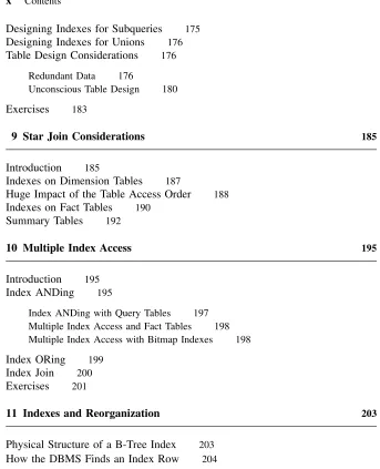
This recommendation is often made in relational literature, usually based on the assumption that only root pages stay in memory. With current processors even when all nonleaf pages are in the database buffer pool, each index level could add as much as 50 microseconds (µs) of central processing unit (CPU) time to an index scan. If a nonleaf page isnot in the database buffer pool, but is found in the read cache of the disk server, the elapsed time for reading the page may be about 1 millisecond (ms). These values should be contrasted with the time taken by a random read from a disk drive, perhaps 10 ms. To see what this effectively means, we will take a simple illustration.
The index shown in Figure 1.1 corresponds to a 100-million-row table. There are 100 million index rows with an average length of 100 bytes. Taking the distributed free space into account, there are 35 index rows per leaf page. If the DBMS does not truncate the index keys in the nonleaf pages, the number of index entries in these pages is also 35.
The probable distribution of these pages as shown in Figure 1.1, together with their size, can be deduced as follows:
100,000,000 index rows
2 entries 1 page
85,500 nonleaf pages 70 entries 2 pages
Leaf
2400 entries 70 pages
83,000 entries 2,400 pages
2,900,000 entries 83,000 pages
[image:24.441.53.300.425.599.2]2,900,000 leaf pages
ž Theindex in total holds about 3,000,000 4 K pages, which requires 12 GB of disk space.
ž The total size of theleaf pagesis 2,900,000×4 K, which is almost 12 GB. It is reasonable to assume that these will normally be read from a disk drive (10 ms).
ž The size of thenext level is 83,000×4 K, which is 332 megabytes (MB); if the index is actively used, then these pages may stay in the read cache (perhaps 64 GB in size) of the disk server, if not in the database buffer pool (say 4 GB for index pages).
ž The upper levels, roughly 2500×4 K=10 MB, will almost certainly remain in the database buffer pool.
Accessingany of these 100,000,000 index rows in this six-level index will then take between 10 and 20 ms. This is true even if many index rows have been added and the index is disorganized, but more about this in Chapter 11. Consequently, it makes little sense to set arbitrary limits to the number of levels.
Myth 2: No More Than Six Indexes per Table
In its positive attitude toward indexes, the Oracle SQL Tuning Pocket Reference (2) by Mark Gurry is an agreeable exception to the comments made earlier. As the title implies, the book focuses on helping the Oracle 9i optimizers, but it also criticizes standards that set an upper limit for the number of indexes per table on page 63:
I have visited sites which have a standard in place that no table can have more than six indexes. This will often cause almost all SQL statements to run beautifully, but a handful of statements to run badly, and indexes can’t be added because there are already six on the table.
. . .
My recommendation is to avoid rules stating a site will not have any more than a certain number of indexes.
. . .
The bottom line is that all SQL statements must run acceptably. There is ALWAYS a way to achieve this. If it requires 10 indexes on a table, then you should put 10 indexes on the table.
Myth 3: Volatile Columns Should Not Be Indexed
the index had four levels; three for the original, two nonleaf and one leaf, together with a further three for the new. When a random disk read took 30 ms, moving one index row could add 6×30 ms=180 ms to the response time of the update transaction. It is hardly surprising that volatile columns were seldom indexed.
These days whenthree levels of a four-level index, the nonleaf pages, stay in memory and a random read from a disk drive takes 10 ms, the corresponding time becomes 2×10 ms=20 ms. Furthermore, many indexes are multicolumn indexes, called compound or composite indexes, which often contain columns that make the index key unique. When a volatile column is the last column of such an index, updating this volatile columnnever causes a move to another leaf page; consequently, with current disks, updating the volatile column adds only 10 ms to the response time of the update transaction.
Example
A few years ago, the DBAs of a well-tuned DB2 installation having an aver-age local response time of0.2 s, started transaction-level exception monitoring. Immediately, they noticed that a simple browsing transaction regularly took more than30 s; the longest observed local response time wasa couple of minutes. They quickly traced the problem to inadequate indexing on a 2-million-row table. Two problems were diagnosed:
ž A volatile column STATUS, updated up to twice a second, was absent from the index, although it was anobvious essential requirement. A predicate using the column STATUS was ANDed to five other predicates in the WHERE clause.
ž An ORDER BY required a sort of the result rows.
These two index design decisions had been made consciously, based on widely used recommendations. The column STATUS was much more volatile than most of the other columns in this installation. This is why the DBAs had not dared to include it in the index. They were also afraid that an extra index, which would have eliminated the sort, would have caused problems with INSERT performance because the insert rate to this table was relatively high. They were particularly worried about theload on the disk drive.
Following the realization of the extent of the problem caused by these two issues, rough estimates of the index overhead were made, and they decided to create an additional index containing the five columns, together with STATUS at the end. This new index solved both problems. The longest observed response time went down from a couple of minutes to less than a second. The UPDATE and INSERT transactions were not compromised and the disk drive containing the new index was not overloaded.
Disk Drive Utilization
is much higher than it was 20 years ago. A reasonable request for a new index should not be rejected intuitively. With current disks, an indexed volatile column may become an issue only if the column is updated perhapsmore than 10 times a second; such columns are not very common.
SYSTEMATIC INDEX DESIGN
The first attempts toward an index design method originate from the 1960s. At that time, textbooks recommended a matrix for predicting how often each field (column) is read and updated and how often the records (rows) containing these fields are inserted and deleted. This led to a list of columns to be indexed. The indexes were generally assumed to have only a single column, and the objective was to minimize the number of disk input/outputs (I/Os) during peak time. It is amazing that this approach is still being mentioned in recent books, although a few, somewhat more realistic writers, do admit that the matrix should only cover the most common transactions.
Thiscolumn activity matrix approachmay explain the column-oriented think-ing that can be found even in recent textbooks and database courses, such as consider indexing columns with these properties andavoid indexing columns with those properties.
In the 1980s, the column-oriented approach began to lose ground to a response-oriented approach. Enlightened DBAs started to realize that the objec-tive of indexing should be to make all database calls fast enough, given the hardware capacity constraints. The pseudo-relational DBMS of IBM S/38 (later AS/400, then the iSeries) was the vanguard of this attitude. It automatically built a good index for each database call. This worked well with simple applications. Today, many products propose indexes for each SQL call, but indexes are not created automatically, apart from primary key indexes and, sometimes, foreign key indexes.
As applications became more complex and databases much larger, the impor-tance and complexity of index design became obvious. Ambitious projects were undertaken to develop tools for automating the design process. The basic idea was to collect a sample of production workload and then generate a set of index candidates for the SELECT statements in the workload. Simple evaluation for-mulas or a cost-based optimizer would then be used to decide which indexes were the most valuable. This sort of product has become available over the last few years but has spread rather slower than expected. Possible reasons for this are discussed in Chapter 16.
1
2
Detect SELECT statements that are too slow due to inadequate indexing
Worst input: Variable values leading to the longest elapsed time
Design indexes that make all SELECT statements fast enough
Table maintenance (INSERT, UPDATE,
DELETE) must be fast enough as well Figure 1.2 Systematic index design.
The first attempts to detect inadequate indexing at design time were based on hopelessly complex prediction formulas, sometimes simplified versions of those used by cost-based optimizers. Replacing calculators with programs and graphical user interfaces did not greatly reduce the effort. Later, extremely simple formulas, like the QUBE, developed in IBM Finland in the late 1980s, or a simple estimation of the number of random I/Os were found useful in real projects. The Basic Question proposed by Ari Hovi was the next and probably the ultimate step in this process. These two ideas are discussed in Chapter 5 and widely used throughout this book.
Methods for improving indexesafter production cutover developed signifi-cantly in the 1990s. Advanced monitoring software forms a necessary base to do this, but an intelligent way to utilize the massive amounts of measurement data is also essential.
This second task of systematic index design went unrecognized for a long time. The SELECTs found in textbooks and course material were so unreal-istically simple that the best index was usually obvious. Experience with real applications has taught, however, that even harmless looking SELECTs, par-ticularly joins, often have a huge number of reasonable indexing alternatives. Estimating each alternative requires far too much effort, and measurements even more so. On the other hand, even experienced database designers have made numerous mistakes when relying on intuition to design indexes.
This is why there is a need for an algorithm to design the best possible index for a given SELECT. The concepts of a three-star index and the related index candidates, which are considered in Chapter 4, have proved helpful.
Chapter
2
Table and Index Organization
ž The physical organization of indexes and tables
ž The structure and use of the index and table pages, index and table rows, buffer pools, and disk cache
ž The characteristics of disk I/Os, random and sequential
ž Assisted random and sequential reads: skip-sequential, list prefetch, and data block prefetching
ž The significance of synchronous and asynchronous I/Os
ž The similarities and differences between database management systems
ž Pages and table clustering, index rows, index-only tables, and page adjacency
ž The very confusing but important issue of the termcluster
ž Alternatives to B-tree indexes
ž Bitmap indexes and hashing
INTRODUCTION
Before we are in a position to discuss the index design process, we need to understand how indexes and tables are organized and used. Much of this, of course, will depend on the individual relational DBMS; however, these all rely on broadly similar general structures and principles, albeit using very different terminology in the process.
In this chapter we will consider the fundamental structures of the relational objects in use; we will then discuss the performance-related issues of their use, such as the role of buffer pools, disks and disk servers, and how they are used to make the data available to the SQL process.
Once we are familiar with these fundamental ideas, we will be in a position, in the next chapter, to consider the way these relational objects are processed to satisfy SQL calls.
This chapter is merely an introduction. Considerably more detail will be provided throughout the book at a time when it is more appropriate. At the end
Relational Database Index Design and the Optimizers, by Tapio Lahdenm¨aki and Michael Leach Copyright2005 John Wiley & Sons, Inc.
of the book, a glossary is provided that summarizes all the terms used throughout the text.
Index and Table Pages
Index and table rows are grouped together in pages; these are often 4K in size, this being a rather convenient size to use for most purposes, but other page sizes may be used. Fortunately, as far as index design is concerned, this is not an important consideration other than that the page size will determine the number of index and table rows in each page and the number of pages involved. To cater for new rows being added to tables and indexes, a certain proportion of each page may be left free when they are loaded or reorganized. This will be considered later.
Buffer pools and I/O activity (discussed later) are based on pages; for example, an entire page will be read from disk into a buffer pool. This means that several rows, not just one, are read into the buffer pool with a single I/O. We will also see that several pages may be read into the pool by just one I/O.
INDEX ROWS
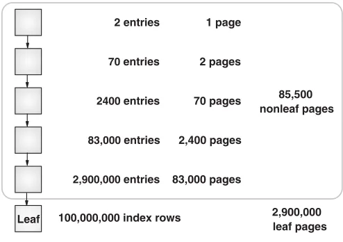
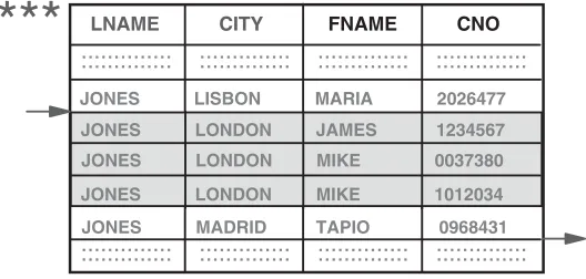
An index row is a useful concept when evaluating access paths. For a unique index, such as the primary key index CNO on table CUST, it is equivalent to an index entry in the leaf page (see Fig. 2.1); the column values are copied from the table to the index, and a pointer to the table row added. Usually, the table page number forms a part of this pointer, something that should be kept in mind for a later time. For anonuniqueindex, such as the index CITY on table CUST, the index rows for a particular index value should be visualized as individual index entries, each having the same CITY value, but followed by a different pointer value. What isactually stored in a nonunique index is, in most cases, one CITY value followed by several pointers. The reason why it isuseful to visualize these as individual index entries will become clear later.
1 3 7
8
20 12
39 33 21 7
20 39
Leaf pages Nonleaf pages
Continue until last level
[image:31.441.52.294.476.609.2]single page
INDEX STRUCTURE
The nonleaf pages always contain a (possibly truncated) key value, the highest key together with a pointer, to a page at the next lower level, as shown in Figure 2.1. Several index levels may be built up in this way, until there is only a single page, called theroot page, at the top of the index structure. This type of index is called a B-tree index (a balanced tree index) because the same number of nonleaf pages are required to find each index row.
TABLE ROWS
Each index row shown in Figure 2.1 points to a corresponding row in the table; the pointer usually identifies the page in which the row resides together with some means of identifying its position within the page. Each table row contains some control information to define the row and to enable the DBMS to handle insertions and deletions, together with the columns themselves.
The sequence in which the rows are positioned in the table, as a result of a table load or row inserts,may be defined so as to be the same as that ofone of its indexes. In this case, as the index rows are processed, one after another in key sequence, so the corresponding table rows will be processed, one after another in the same sequence. Both index and table are then accessed in a sequential manner that, as we will see shortly, is a very efficient process.
Obviously,only one of the indexes can be defined to determine the sequence of the table rows in this way. If the table is being accessed viaany other index, as the index rows are processed, one after another in key sequence, the corre-sponding rows willnot be held in the table in the same sequence. For example, the first index row may point to page 17, the next index row to page 2, the next to page 85, and so forth. Now, although the index is still being processed sequentially and efficiently, the table is being processed randomly and much less efficiently.
BUFFER POOLS AND DISK I/OS
arises. For now we must simply be aware of the relative costs involved in accessing index or table rows from pages that may or may not be stored in the buffer pools.
Reads from the DBMS Buffer Pool
If an index or table page is found in the buffer pool, the only cost involved is that of the processing of the index or table rows. This is highly dependent on whether the row is rejected or accepted by the DBMS, the former incurring very little processing, the latter incurring much more as we will see in due course.
Random I/O from Disk Drives
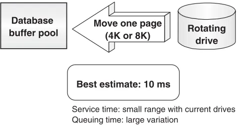
Figure 2.2 shows the enormous cost involved in having to wait for a page to be read into the buffer pool from a disk drive.
Again, we must remember that a page will contain several rows; we may be interested in all of these rows, just a few of them, or even only a single row—the cost will be the same, roughly 10 ms. If the disk drives are heavily used, this figure might be considerably increased as a result of having to wait for the disk to become available. In computing terms, 10 ms is an eternity, which is why we will be so interested in this activity throughout this book.
It isn’t really necessary to understand how this 10 ms is derived, but for those readers who like to understand where numbers such as this come from, Figure 2.3 breaks it down into its constituent components. From this we can see that we are assuming the disk would actually be busy for about 6 out of the 10 ms. The transfer time of roughly 1 ms refers to the movement of the page from the disk server cache into the database buffer pool. The other 3 ms is an estimate of the queuing time that might arise, based on disk activity of, say, 50 reads per second. These sort of figures would equally apply to directly attached drives; all the figures will, of course, vary somewhat, but we simply need to keep in mind a rough, but not unreasonable, figure of 10 ms.
Rotating drive Move one page
(4K or 8K) Database
buffer pool
Best estimate: 10 ms
[image:33.441.52.292.466.593.2]Service time: small range with current drives Queuing time: large variation
Depends on drive busy
Q = (u / (1–u)) × S
Q = Average queuing time u = Average drive busy S = Average service time
50 random reads a second
u = 50 read/s × 0.006 s/read = 0.3
Q = (0.3 /(1- 0.3)) × 6 ms = 3 ms
Queuing (Q) 3 ms Seek 4 ms Half a rotation 2 ms Transfer 1 ms Total I/O time 10 ms
S = Service time
One random read keeps a drive busy for 6 ms
Figure 2.3 Random I/O from disk drive—2.
Move one page (4K or 8K) Database
buffer pool
Estimate: 1 ms
Read cache
Depends on many factors
Figure 2.4 Read from disk server cache.
Reads from the Disk Server Cache
Fortunately, disk servers in use today provide their own memory (or cache) in order to reduce this huge cost in terms of elapsed time. Figure 2.4 shows the read of a single table or index page (again equivalent to reading a number of table or index rows) from the cache of the disk server. Just as with the buffer pools, the disk server is trying to hold frequently used data in memory (cache) rather than incurring the heavy disk read cost. If the page required by the DBMS is not in the buffer pool, a read is issued to the disk server who will check to see if it is in the server cache and only perform a read from a disk drive if it is not found there. The figure of 10 ms may be considerably reduced to a figure as low as 1 ms if the page is found in the disk server read cache.
Full table scan Full index scan Index slice scan
Scan table rows via clustering index
Estimate: 0.1 ms per 4K page
Large range...should be measured
40 MB/s
Figure 2.5 Sequential reads from disk drives.
Sequential Reads from Disk Drives
So far, we have only considered reading a single index or table page into the buffer pool. There will be many occasions when we actually want to read several pages into the pool and process the rows in sequence. Figure 2.5 shows the four occasions when this will apply. The DBMS will be aware that several index or table pages should be read sequentially and will identify those that are not already in the buffer pool. It will then issue multiple-page I/O requests, where the number of pages in each request will be determined by the DBMS; only those pages not already in the buffer pool will be read because those that are already in the pool may contain updated data that has not yet been written back to disk.
There are two very important advantages to reading pages sequentially:
ž Reading several pages together means that the time per page will be reduced; with current disk servers, the value may be as low as 0.1 ms for 4K pages (40 MB/s).
ž Because the DBMS knows in advance which pages will be required, the reads can be performed before the pages are actually requested; this is called prefetch.
The terms index slice and clustering index referred to in Figure 2.5 will be addressed shortly. Terms used to refer to the sequential reads described above include Sequential Prefetch, Multi-Block I/Os, and Multiple Serial Read-Ahead Reads.
Assisted Random Reads
Automatic Skip-Sequential
By definition, an access pattern will be skip-sequential if a set of noncontiguous rows are scanned in one direction. The I/O time per row will thus be automatically shorter than with random access; the shorter the skips, the greater the benefit. This would occur, for example, when table rows are being read via a clustering index and index screening takes place, as we will see in due course. This benefit can be enhanced in two ways:
1. The disk server may notice that access to a drive is taking place sequen-tially, or almost sequensequen-tially, and starts to read several pages ahead. 2. The DBMS may notice that a SELECT statement is accessing the pages
of an index or table sequentially, or almost sequentially, and starts to read several pages ahead; this is called dynamic prefetch in DB2 for z/OS.
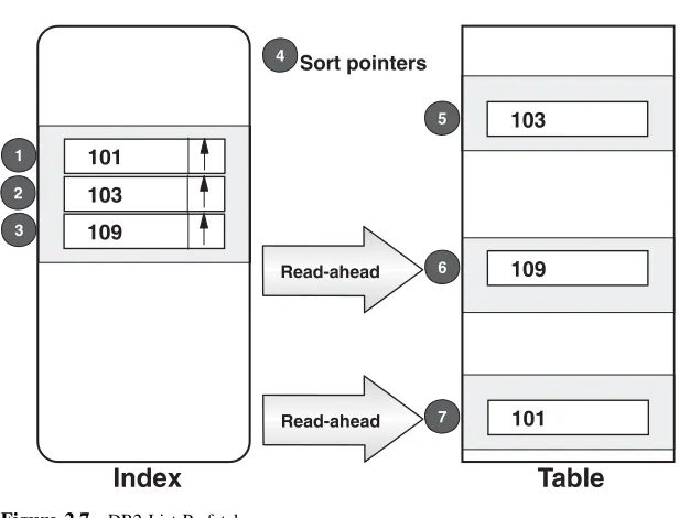
List Prefetch
In the previous example, this benefit was achieved simply as a result of the table and index rows being in the same sequence. DB2 for z/OS is in fact able to create skip-sequential access even when this isnot the case; to do this, it has to access all the qualifying index rows and sort the pointers into table page sequence before accessing the table rows. Figures 2.6 and 2.7 contrast an access path that does not use list prefetch with one that does, the numbers indicating the sequence of events.
103
109 101
103
109
101 4
6
2 1
3
5
Index
Table
Page
103
109 101
103
109
101 5
6
7 1
2
3
Index
Table
4 Sort pointers
Read-ahead
[image:37.441.52.360.59.294.2]Read-ahead
Figure 2.7 DB2 List Prefetch.
Data Block Prefetching
This feature is used by Oracle, again when the table rows being accessed are not in the same sequence as the index rows. In this case, however, as shown in Figure 2.8, the pointers are collected from the index slice and multiple random I/Os are started to read the table rows in parallel. If the table rows represented by steps 4, 5, and 6 reside on three different drives, all three random I/Os will be performed in parallel. As with list prefetch, we could use Figures 2.6 and 2.8 to contrast an access path that does not use data block prefetching with one that does.
Before we leave assisted random reads, it might be worth considering the order in which a result set is obtained. An index could provide the correct sequence automatically, whereas the above facilities could destroy this sequence before the table rows were accessed, thereby requiring a sort.
Comment
Throughout this book, we will refer to three types of read I/O operations: syn-chronous, sequential, and assisted random reads; in order to make the estimation process usable, initially only the first two types will be addressed, but Chapter 15 will discuss assisted random read estimation in some detail.
103 109 101
103
109
101 5
6
4 1
2
3
Index
Table
Read-ahead Read-ahead
Figure 2.8 Oracle data block prefetching.
Assisted Sequential Reads
When a large table is to be scanned, the optimizer may decide to activate par-allelism; for instance, it may split a cursor into several range-predicate cursors, each of which would scan one slice. When several processors and disk drives are available, the elapsed time will be reduced accordingly. Again we will put this to one side until we come to Chapter 15. Please note that the term assisted sequential reads is again not one that is used by any of the DBMSs.
Synchronous and Asynchronous I/Os
Having discussed these different access techniques, it will be appropriate now to ensure we fully appreciate one final consideration, synchronous and asynchronous I/Os as shown in Figure 2.9.
The term synchronous I/O infers that while the I/O is taking place, the DBMS is not able to continue any further; it is forced to wait until the I/O has completed. With a synchronous read, for example, we have to identify the row required (shown as “C” to represent the first portion of CPU time in the figure), access the page and process the row (shown as the second portion of CPU time), each stage waiting until the previous stage completes.
Synchronous read Random read Synchronous write
Log write
Asynchronous read
Sequential prefetch Assisted random read
Asynchronous write Database writes
I/O
I/O
C C
C C C Sync I/O
C Sync I/O C
I/O I/O
Figure 2.9 Synchronous and asynchronous I/O.
before the pages are actually required for processing. Each group of pages being prefetched and processed in this way is shown in Figure 2.9; note that a syn-chronous read kick-starts the whole prefetch activity before the first group of pages is prefetched to minimize the first wait.
When the DBMS requests a page, the disk system may read the next few pages as well into a disk cache (anticipating that these may soon be requested); this could be the rest of the stripe, the rest of the track, or even several stripes (striping is described shortly). We call this Disk Read Ahead.
Most database writes are performed asynchronously such that they should have little effect on performance. The main impact they do have is to increase the load on the disk environment, which in turn may affect the performance of the read I/Os.
HARDWARE SPECIFICS
At the time of writing, the disk drives used in database servers do not vary much with regard to their performance characteristics. They run at 10,000 or 15,000 rotations per minute and the average seek time is 3 or 4 ms. Our suggested estimate for an average random read from a disk drive (10 ms)—including drive queuing and the transfer time from the server cache to the pool—is applicable forall current disk systems.
In addition to the I/O time estimates, the cost of disk space and memory influences index design.
Local disk drives provide physical data storage without the additional func-tion provided by disk servers (such as fault tolerance, read and write cache, striping, and so forth), for a very low price.
Disk servers are computers with several processors and a large amount of memory. The most advanced disk servers are fault tolerant: All essential com-ponents are duplicated, and the software supports a fast transfer of operations to a spare unit. A high-performance fault tolerant disk server with a few terabytes may cost $2 million. The cost per gigabyte, then, is in the order of U.S.$500 (purchase price) or U.S.$50 per month (outsourced hardware).
Both local disks and disk servers employ industry-standard disk drives. The largest drives lead to the lowest cost per gigabyte; for example, a 145-GB drive costs much less than eight 18-GB drives. Unfortunately, they also imply much longer queuing times than smaller drives with a given access density (I/Os per gigabyte per second).
The cost of memory has been reduced dramatically over the last few years as well. A gigabyte of random access memory (RAM) for Intel servers (Windows and Linux) now costs about $500 while the price for RISC (proprietary UNIX and Linux) and mainframe servers (z/OS and Linux) is on the order of U.S.$10,000 per gigabyte. With 32-bit addressing, the maximum size of a database buffer pool might be a gigabyte (with Windows servers, for example), and a few gigabytes for mainframes that have several address spaces for multiple buffer pools. Over the next few years, 64-bit addressing, which permits much larger buffer pools, will probably become the norm. If the price for memory (RAM) keeps falling, database buffer pools of 100 gigabytes or more will then be common.
The price for the read cache of disk servers is comparable to that of RISC server memory. The main reason for buying a 64-GB read cache instead of 64 GB of server memory is the inability of 32-bit software to exploit 64 GB for buffer pools.
Throughout this book, we will use the following cost assumptions: CPU time $1000 per hour, based on 250 mips per processor Memory $1000 per gigabyte per month
Disk space $50 per gigabyte per month
These are the possible current values for outsourced mainframe installations. Each designer should, of course, ascertain his or her own values, which may be very much lower than the above.
DBMS SPECIFICS
Pages
leaf page. If the average length of the rows in a table is more than one third of the page size, space utilization suffers. Only one row with 2100 bytes fits in a 4K page, for instance. The problem of unusable space is more pronounced with indexes. As new index rowsmust be placed in a leaf page according to the index key value, the leaf pages of many indexes should have free space for a few index rows, after load and reorganization. Therefore, index rows that are longer than 20% of the leaf page may result in poor space utilization and frequent leaf page splits. We have much more to say about this in Chapter 11.
With current disks, one rotation takes 4 ms (15,000 rpm) or 6 ms (10,000 rpm). As the capacity of a track is normally greater than 100 kilobytes (kb), the time for a random read is roughly the same for 2K, 4K, and 8K pages. It is essential, however, that the stripe size on RAID disks is large enough for one page; otherwise, more than one disk drive may have to be accessed to read a single page.
In most environments today, sequential processing brings several pages into the buffer pool with one I/O operation—several pages may be transferred with one rotation, for instance. The page size does not then make a big difference in the performance of sequential reads.
SQL Server 2000 uses a single page size for both tables and indexes: 8K. The maximum length of an index row is 900 bytes.
Oracle uses the term block instead of page. The allowed values for BLOCK SIZE are 2K, 4K, 8K, 16K, 32K, and 64K, but some operating systems may limit this choice. The maximum length of an index row is 40% of BLOCK SIZE. In the interests of simplicity, we trust Oracle readers will forgive us if we use the termpage throughout this book.
DB2 for z/OS supports 4K, 8K, 16K, and 32K pages for tables but only 4K pages for indexes. The maximum length for index rows is 255 bytes in V7, but this becomes 2000 bytes in V8.
DB2 for LUW allows page sizes of 4K, 8K, 16K, and 32K for both tables and indexes. The upper limit for the index row length is 1024 bytes.
Table Clustering
Index Rows
The maximum number of columns in an index varies across the current DBMSs: SQL Server 16, Oracle 32, DB2 for z/OS 64, and DB2 for LUW 16 (refer to Chapter 12 for more detail).
Indexing variable-length columns have limitations in some products. If only fixed-length index rows are supported, the DBMS may pad an index column to the maximum length. As variable-length columns are becoming more common (because of JAVA, for instance)—even in environments in which they were rarely used in the past—support for variable-length index columns (and index rows) is now the norm in the latest releases. DB2 for z/OS, for instance, has full support for variable-length index columns in V8.
Normally, all columns copied to an index form the index key, which deter-mines the order of the index entries. In unique indexes, an index entry is the same as an index row. With nonunique indexes, there is an entry for each distinct value of the index key together with a pointer for each of the duplicate table rows; this pointer chain is normally ordered by the address of the table row. DB2 for LUW, for instance, allows nonkey columns at the end of an index row. In addition to the above, each index entry requires a certain amount of control information, used, for example, to chain the entries in key sequence; throughout this book, this control information will be assumed, for the purpose of determining the number of index rows per page, to be about 10 bytes in length.
Table Rows
We have already seen that some DBMSs, for instance, DB2 for z/OS, DB2 for LUW, Informix, and Ingres, support a clustering index, which affects the placement of inserted table rows. The objective is to keep the order of the table rows as close as possible to the order of the rows in the clustering index. If there is no clustering index, the inserted table rows are placed in the last page of the table or to any table page that has enough free space.
Some DBMSs, for example, Oracle and SQL Server, do not support a clus-tering index that influences the choice of table page for an inserted table row. However, with any DBMS, the table rows can be maintained in the required order by reorganizing the table frequently; by reading the rows via a particular index (the index that determines the required order) before the reload or by sorting the unloaded rows before the reload.
Oracle and SQL Server provide an option for storing the table rows in the index as shown in the next section. More information is provided in Chapter 12.
Index-Only Tables
Some DBMSs have the option of avoiding the need for the table. The leaf pages of one of the indexes then effectively contain the table rows.
In Oracle, this option is called an index-organized table, and the index con-taining the table rows is called the primary index. In SQL Server, the table rows are stored in an index created with the option CLUSTERED. In both cases, the other indexes (called secondary indexes in Oracle and unclustered indexes in SQL Server) point to the index that contains the table rows.
The obvious advantage of index-only tables is a saving in disk space. In addition, INSERTs, UPDATEs, and DELETEs are a little faster because there is one less page to modify.
There are, however, disadvantages relating to the other indexes. If these point to the table row using a direct pointer (containing the leaf page number), a leaf page split in the primary (clustered) index causes a large number of disk I/Os for the other indexes. Any update to the primary index key that moves the index row, forces the DBMS to update the index rows pointing to the displaced index row. This is why SQL Server, for instance, now uses the key of the primary index as the pointer to the clustered index. This eliminates the leaf page split overhead, but the unclustered indexes become larger if the clustered index has a long key itself. Furthermore, any access via a nonclustered index goes through two sets of nonleaf pages; first, those of the unclustered index and then those of the clustered index. This overhead is not a major issue as long as the nonleaf pages stay in the buffer pool.
The techniques presented in this book apply equally well to index-only tables, although the diagrams always show the presence of the table.If index-only tables are being used, the primary (clustered) table should be considered as a clustering index that is fat for all SELECTs. This last statement may not become clear until Chapter 4 has been considered. The order of the index rows is determined by the index key. The other columns are nonkey columns.
Note that in SQL Server the clustered index does not have to be theprimary key index. However, to reduce pointer maintenance, it is a common practice to choose an index whose key is not updated, such as a primary or a candidate key index. In most indexes (the nonkey column option will be discussed later), all index columns make up the key, so it may be difficult to find other indexes in which no key column is updated.
Page Adjacency
Are the logically adjacent pages (such as leaf page 1 and leaf page 2) physically adjacent on disk? Sequential read would be very fast if they are (level 2 in Fig. 2.10).
Three levels:
Read one page, get many rows Read one track, get many pages
Disk server reads ahead from drives to read cache
Level 1 automatic
If 10 rows per 4K page, then I/O time = 1 ms per row Level 2 support by DBMS or disk system May reduce sequential I/O time per row to 0.1 ms Level 3 support by Disk Server
May reduce sequential I/O time per row to 0.01 ms Figure 2.10 Page adjacency.
10 rows per page and a random I/O takes 10 ms, the I/O time for a sequential read is then 1 ms per row.
SQL Server allocates space for indexes and tables in chunks of eight 8K pages. DB2 for z/OS allocates space in extents; an extent may consist of many megabytes, all pages of a medium-size index or table often residing in one extent. The logically adjacent pages are then physically next to each other. In Oracle (and several other systems) the placement of pages depends on file options chosen.
Many databases are now stored on RAID 5 or RAID 10 disks. RAID5 pro-videsstripingwithredundancy. RAID 10, actually RAID 1+RAID 0, provides stripingwithmirroring.
The termsredundancyandmirroringare defined in the glossary. RAID strip-ing means storing the first stripe of a table or index (e.g., 32K) on drive 1, the second stripe on drive 2, and so on. This obviously balances the load on a set of drives, but how does it affect sequential performance? Surprisingly, the effect may be positive.
Let us consider a full table scan where the table pages are striped over seven drives. The disk server may nowread ahead from seven drives in parallel. When the DBMS asks for the next set of pages, they are likely to be already in the read cache of the disk server. This combination of prefetch activity may bring the I/O time down to 0.1 ms per 4K page (level 3 in Fig. 2.10). The 0.1-ms figure is achievable with fast channels and a disk server that is able to detect that a file is being processed sequentially.
Alternatives to B-tree Indexes
Bitmap Indexes
Bitmap indexes consist of a bitmap (bit vector) for each distinct column value. Each bitmap has one bit for every row in the table. The bit is on if the related row has the value represented by the bitmap.
ORing (covered in Chapters 6 and 10) bitmap indexes is very fast, even when there are hundreds of millions of table rows. The corresponding operation with B-tree indexes requires collecting a large number of pointers and sorting large pointer sets.
On the other hand a B-tree index, containing the appropriate columns, elimi-nates table access. This is important because random I/Os to a large table are very slow (about 10 ms). With a bitmap index, the table rowsmust be accessed unless the SELECT list contains only COUNTs. Therefore, the total execution time using a bitmap index may bemuch longer than with a tailored, (fat) B-tree index.
Bitmap indexes should be used when the following conditions are true: 1. The number of possible predicate combinations is so large that designing
adequate B-tree indexes is not feasible.
2. The simple predicates have a high filter factor (considered in Chapter 3), but the compound predicate (WHERE clause) has a low filter factor—or the SELECT list contains COUNTs only.
3. The updates are batched (no lock contention).
Hashing
Hashing—or randomizing—is a fast way to retrieve a single table row whose primary key value is known. When the row is stored, the table page is chosen by using a randomizer, which converts the primary key value into a page number between 1 and N. If that page is already full, the row is placed in another page, chained to the home page. When a SELECT . . . WHERE PK=:PK is issued, the randomizer is used again to determine the home page number. The row is either found in that page or by following the chain that starts on that page.
Randomizers were commonly used in nonrelational DBMSs such as IMS and IDMS. When the area size (N) was right—corresponding to about 70% space utilization, the number of I/Os to retrieve a record could have been as low as 1.1, which was very low compared to an index (a three-level index at that time could require two I/Os—plus a third to access the record itself). However, the space utilizations required constant monitoring and adjustments. When many records were added, the overflow chains grew and the number of I/Os increased dramatically. Furthermore, range predicates were not supported. Oracle provides an option for the conversion of a primary key value to a database page number by hashing.
Many Meanings of Cluster
Cluster is a term that is widely used throughout relational literature. It is also a source of much confusion because its meaning varies from product to product.