Distributed processing for statistical data mining

Full text

(1)ResearchOnline@JCU. This file is part of the following reference:. Sim, Nigel Graham Donald (2012) Distributed processing for statistical data mining. PhD thesis, James Cook University. Access to this file is available from:. http://eprints.jcu.edu.au/25231 The author has certified to JCU that they have made a reasonable effort to gain permission and acknowledge the owner of any third party copyright material included in this document. If you believe that this is not the case, please contact [email protected] and quote http://eprints.jcu.edu.au/25231.

(2) Distributed Processing for Statistical Data Mining. Thesis submitted by Nigel Graham Donald Sim BE (Hons)/BSc. For the degree of Doctor of Philosophy In Information Technology at James Cook University, Townsville. i.

(3) STATEMENT OF ACCESS. I, the undersigned author of this work, understand that James Cook University will make this thesis available for use within the University Library and, via the Australian Digital Theses network, for use elsewhere. I understand that, as an unpublished work, a thesis has significant protection under the Copyright Act and; I do not wish to place any further restriction on access to this work. 15 March 2012 Signature. Date. ii.

(4) STATEMENT ON SOURCES DECLARATION I declare that this thesis is my own work and has not been submitted in any form for another degree or diploma at any university or other institution of tertiary education. Information derived from the published or unpublished work of others has been acknowledged in the text and a list of references is given.. 15 March 2012 Signature. Date. iii.

(5) ELECTRONIC COPY. I the under-signed, the author of this work, declare that the electronic copy of this thesis provided by James Cook University Library is an accurate copy of the print thesis submitted, within the limits of the technology available.. 15 March 2012 Signature. Date. iv.

(6) STATEMENT ON CONTRIBUTIONS OF OTHERS. The research described and presented in this thesis was undertaken by the author under the supervision of Professor Ian Atkinson and Professor Danny Coomans, both of whom provided editorial and academic advice. Financial support in the form of a scholarship was gratefully received from the School of Maths and Physics, and the School of Information Technology. Further support was received from the Graduate Research School in the form of research grants, and from the Australian Mathematical Sciences Institute, Australian Partnership for Advanced Computing, and the International Society for Business and Industrial Statistics in the form of conference travel grants. I would also like to thank Dr Dmitry Konovalov, Dr Yvette Everingham and Dr Timothy Hancock for their discussions and expertise in the fields of data mining and statistics.. v.

(7) ACKNOWLEDGEMENTS Firstly I would like to thank my parents, Helen and Robin, and brother Russell for their continued support and encouragement through the ups and downs encountered on the path to completing this project. Additionally, I owe a great debt of gratitude to my supervisors Professor Ian Atkinson and Professor Danny Coomans for their guidance, inspirational advice, and ability to help me see the bigger picture when doubts abounded. I would like to also thank Gavin and Carol Blackman for their personal encouragement and advice in constructing scientific argument and prose. Finally I would like to thank my friends and colleagues who have contributed to this thesis through their encouragement, discussion, friendship and feedback, with special thanks to: David Laing, David Browning, Adrian Knack and Angela Hughes.. vi.

(8) ABSTRACT The use of information technology (IT) in scientific investigations is now commonplace, due largely to the increased efficiency of IT procedures in managing and organising data sets now able to be generated through technologically aided data recording methods. While such data sets can be advantageous to investigative work, the size and complexity of these pose special challenges to exploring and revealing their information content. Data mining procedures offer many general purpose tools that can be used to explore large volumes of data to find patterns and structures within the data sets that are able to relate response variables to observations. However data mining techniques need to be matched to the attributes of the input data sets. In general, data sets with larger numbers of input variables require robust and sophisticated techniques to reliably identify patterns and processes within the data structures. Additionally, more sophisticated data mining techniques take more computational time to execute than simple data mining techniques. However, some computational problems typical of data mining are amenable to being easily divided into discrete tasks able to be executed independently, in parallel across many computational resources. The project reported in this thesis generated the components of an eResearch framework. A workflow language was developed to capture the critical aspects of a data mining process, allowing the parallel components to be exploited. Subsequent development of a distributed computing framework enabled leverage of existing data mining tools such as MATLAB and R to perform actual data processing. This distributed computing framework controls movement of data and execution of tasks based on the workflow submitted by the practitioner initiating the workflow. The coordinating element within the distributed computing framework is a new task scheduling algorithm, termed “Neglected”. This algorithm is the major research contribution of this project. “Neglected”is a task matching algorithm that optimises total execution time of an experiment by minimising the unnecessary movement of data. This is achieved by matching resources to tasks, where a task's estimated completion time is within a margin of that task's best matching option. The “Neglected” task scheduling algorithm was tested in simulation against a commonly used distributed computing scheduling algorithm, the “MinMin” greedy scheduler. The new algorithm significantly outperformed “MinMin” in terms of data transfer, and in most scenarios it also outperformed in terms of total compute time. This is attributed to the reduced transfer overhead required to satisfy the tasks assigned to each resource. The “Neglected” scheduling algorithm offers improved efficiency in the use of resources and improved time to solution for workflow execution. This, together with the data mining workflow and execution framework, extend and improve overall efficiency, robustness and repeatability in the analysis of new and existing data sets by computationally intensive data mining techniques.. vii.

(9) Table of Contents 1. Introduction......................................................................................................................... 1 1.1. eScience and the Grid.................................................................................................... 3 1.2. Data mining................................................................................................................... 5 1.3. Scheduling Distributed Computing Execution.............................................................. 7 1.4. Project Summary........................................................................................................... 8 1.5. Contributions................................................................................................................. 8 1.6. Thesis Organisation....................................................................................................... 8 2. Background and Overview............................................................................................... 10 2.1. Robust Data Mining of Large Data sets....................................................................... 11 2.1.1. Cheminformatics – Data mining in Chemistry.................................................... 12 2.1.2. Data Mining as eScience..................................................................................... 13 2.1.3. Efficiently Speeding Up Execution...................................................................... 16 2.1.4. Review of Contemporary Data Mining Techniques............................................. 19 2.1.5. Typical Data Mining Experiments...................................................................... 24 2.1.6. Properties of an eScience Data Mining System.................................................. 27 2.2. Experiment Expression and Management Review...................................................... 28 2.2.1. Expression of a Data Mining Experiment........................................................... 29 2.2.2. Experiment Management – Collection of Experiment Metadata........................ 32 2.3. Deployment and Integration Review........................................................................... 34 2.3.1. Execution of Operations and Applications......................................................... 35 2.3.2. Data Interchange and Conversion...................................................................... 37 2.3.3. Communications and Data Security................................................................... 41 2.3.4. Recoverability..................................................................................................... 42 2.4. Computational Platform Review................................................................................. 43 2.4.1. Survey of Distributed Computing Topologies and Services................................ 44 2.4.2. Master-Slave Execution Model........................................................................... 50 2.4.3. Scheduling Notation............................................................................................ 52 2.4.4. Task Scheduling in Distributed Computing........................................................ 55 2.5. Previous Projects......................................................................................................... 58 2.5.1. Data Mining Services Middleware...................................................................... 59 2.5.2. GridMiner........................................................................................................... 60 2.5.3. Nimrod................................................................................................................ 60 2.5.4. Kepler.................................................................................................................. 61 2.5.5. Taverna............................................................................................................... 62 2.5.6. RapidMiner......................................................................................................... 63 2.5.7. WEKA.................................................................................................................. 63 2.5.8. R Language......................................................................................................... 64 2.5.9. Summary of Previous Projects............................................................................ 65 2.6. Summary..................................................................................................................... 67 3. Distributed workflow, and eScience tool chain............................................................... 68 3.1. Review of Data Mining Experiment Requirements..................................................... 69 3.1.1. General Data Mining Experiment Use Case....................................................... 70 3.2. Experiment Representation......................................................................................... 71 3.2.1. Workflow............................................................................................................. 72 3.2.1.1. Example workflow....................................................................................... 77 3.2.2. Operators............................................................................................................ 78 3.2.3. Data.................................................................................................................... 80. viii.

(10) 3.3. Agent Based Execution System................................................................................... 82 3.3.1. Operator Invocation............................................................................................ 83 3.3.2. Distributed Execution......................................................................................... 85 3.3.2.1. Agent Communications............................................................................... 86 3.3.2.2. Agent Communications Protocol................................................................ 87 3.4. Data Services to Support Distributed Execution......................................................... 89 3.4.1. Agent Data Access Component............................................................................ 91 3.4.2. Data Formats...................................................................................................... 92 3.5. Experiment Metadata and Data Provenance............................................................... 93 3.5.1. Process provenance............................................................................................. 94 3.5.2. Data Provenance................................................................................................. 97 3.5.3. Provenance Storage............................................................................................ 98 3.6. Transforming Syntax Trees into Tasks........................................................................ 99 3.7. Conclusion................................................................................................................. 101 4. Development and Analysis of a New Task Scheduling Algorithm............................... 103 4.1. Survey of Master-Slave Scheduling Heuristics.......................................................... 105 4.2. Scheduling of Heterogeneous Tasks in a Heterogeneous Environment.................... 106 4.2.1. Scheduling for Data Distribution...................................................................... 113 4.3. Validation of systems via simulation frameworks..................................................... 116 4.3.1. Calibration of the simulation............................................................................. 117 4.3.2. Simulation of Allocation Algorithm.................................................................. 119 4.4. Experimental Results................................................................................................. 123 4.6. Utilisation of Resource Parallelism.......................................................................... 133 4.7. Summary.................................................................................................................... 134 5. Predictive modelling for human intestinal absorption of chemical compounds .......135 5.1. Introduction................................................................................................................ 136 5.2. Materials and methods............................................................................................... 137 5.2.1. Experiment......................................................................................................... 141 5.3. Results and discussions............................................................................................. 142 5.4. Workflow and provenance......................................................................................... 146 5.5. Conclusion................................................................................................................. 148 6. Conclusions and Future Work........................................................................................ 149 6.1. eScience: Workflow and Provenance......................................................................... 149 6.2. Distributed Computing.............................................................................................. 150 6.3. Benefits to Data Mining Applications....................................................................... 151 6.4. Outcomes and Contributions..................................................................................... 152 6.5. Future Work............................................................................................................... 153 6.5.1. Resource Scheduling.......................................................................................... 153 6.5.2. Applications...................................................................................................... 154 6.6. Concluding remarks.................................................................................................. 156 Nomenclature....................................................................................................................... 157 References............................................................................................................................. 159 Appendix A - Optimising Ensemble Predictions.............................................................. 175 A.1. Methods and materials.............................................................................................. 176 A.1.1. Heterogeneous ensemble................................................................................... 176 A.1.2. Lasso post-processing....................................................................................... 177 A.1.3. Evolutionary strategies post-processing........................................................... 177 A.1.4. Blood Brain Barrier (BBB) data set ................................................................ 179 A.1.5. Friedman1000................................................................................................... 179 A.2. Results and discussion.............................................................................................. 179 ix.

(11) A.3. Conclusion................................................................................................................ Appendix B - Important Grid Agent Interfaces............................................................... B.1. IAgent.java................................................................................................................. B.2. ITupleStore.java........................................................................................................ B.3. IFileMovement.java.................................................................................................. B.4. IPeerStatus.java......................................................................................................... Appendix C - Workflow XML Schema............................................................................... 181 182 182 183 184 185 187. x.

(12) List of Tables Table 2.1: Summary of cross-validation technique procedures, relating number of iterations required to n=observations and k=testsets............................................................................... 22 Table 2.2: Different classes of distributed resource, and some attributes of these..................47 Table 2.3: Summary of notation used to describe task scheduling.........................................53 Table 2.4: Summary of previous projects covering data mining............................................. 66 Table 3.1: Common provenance attributes about compute resources...................................... 95 Table 3.2: Common provenance attributes supplied by all operators...................................... 96 Table 3.3: Additional provenance information provided by the R operator............................ 96 Table 4.1: GridSim network model comparison results......................................................... 118 Table 4.2: Host configurations for simulation executions...................................................... 121 Table 4.3: Normalised makespan for varying operator run times and repeat values.............124 Table 4.4: Experiment data transfer saturation for the four scheduling algorithms, across the parameter space of operator size, task size and file count..................................................... 126 Table 4.5: Final data placements for scheduling algorithms vs iterations (compute dominated) ............................................................................................................................................... 128 Table 4.6: Final data placements for scheduling algorithms vs iterations (data dominated).130 Table 5.1: Previous performance results for predictive models based in the HIA data set....138 Table 5.2: Top 6 most frequently selected variables by data set using GA-PLS as reported by Hou........................................................................................................................................ 142 Table 5.3: Top 6 variables selected using random forests variable importance measure......143 Table 5.4: Top 6 variables selected using GA-PLS across the MCCV variable selection.....144 Table 5.5: Mean predictive performance of HIA data set descriptors using PLS, SVM and RF predictive models using variables selected by Random Forest.............................................. 145 Table 5.6: Mean predictive performance of HIA data set descriptors using PLS, SVM and RF predictive models using variables selected by GA-PLS........................................................ 145 Table 5.7: Amount of time (serial) spent performing each step of the workflow.................. 147 Table 1: R2 results of the ensemble post-processing techniques on the blood-brain barrier and Friedman1000 data sets................................................................................................... 180. xi.

(13) List of Figures Figure 1.1: High level flow chart of the data mining process, and the outputs produced by it. 5 Figure 2.1: Process of distilling various sources of chemical observations into a table of data, from which a model can be built............................................................................................. 13 Figure 2.2: An experiment is the application of a process on input data and algorithms, to produce output data and an experiment log............................................................................. 15 Figure 2.3: Typical data mining process considered in this thesis........................................... 16 Figure 2.4: Amdahl's law showing the speedup obtained by adding additional resources......18 Figure 2.5: Generic ensemble of independent weighted models............................................. 23 Figure 2.6: Bagging: Ensemble of independent weighted models built on subsets of the data. ................................................................................................................................................. 23 Figure 2.7: Flow chart of cross-validation as applied in data mining...................................... 25 Figure 2.8: Abstract representation of the list of steps for the generalised process that a) data mining practitioners and b) algorithm developers, may use in their work..............................26 Figure 2.9: A typical data mining experiment template exhibiting iteration, nesting of iteration and sequential application of operators..................................................................... 27 Figure 2.10: A computational experiment is comprised of algorithms, data management and experiment management. Workflows provide the experiment management functionality, allowing the application to be more focused and general purpose.......................................... 29 Figure 2.11: Adaption of disparate data sources to provide a consistent interface for the data mining workflow...................................................................................................................... 38 Figure 2.12: Staging data via disk is a simple way of bridging legacy applications to the Grid. ................................................................................................................................................. 40 Figure 2.13: The use of a shim can redirect file access in a way that is transparent to the Application.............................................................................................................................. 41 Figure 2.14: Compute resources potentially available to practitioners within an institution. Includes networks of workstations, Grids and clusters, and commercially provided Cloud resources.................................................................................................................................. 45 Figure 2.15: Grid Resource Broker provides a service to locate and acquire resources, based on market system..................................................................................................................... 48 Figure 2.16: Example Data Grid scenario: Multiple resources located next to computational resources, and controlled by a replica catalogue. The User can request data be replicated between storage resources to provide local access to data by compute resources...................49 Figure 2.17: Master-slave paradigm: Slave compute resources connected via a network perform tasks requested by a master resource......................................................................... 51 Figure 2.18: Abstract algorithm for the master node in a master-slave system........................ 52 Figure 2.19: Abstract algorithm for a slave node in a master-slave system............................. 52 Figure 2.20: Communications between master and slaves during task execution................... 52 Figure 2.21: Impact of decreasing bandwidth (or increasing data size) on makespan............56 Figure 3.1: Experiment document describe data elements, operators and a workflow, which all map to their counterparts in the eScience system.............................................................. 69 Figure 3.2: Top level elements within the experiment document............................................ 72 Figure 3.3: Parameter sweep blocks and subsetting example: Lines 1-4 generate data and write it to a store including variables which indicate the index of the iterators. Lines 5-6 bring those same iterators into scope again, and line 8 uses subsetting to retrieve the data stored in line 4. Method or sub-setting parameter names are shown in italics........................73 Figure 3.4: Illustration of variable scoping. a) Variable x is in scope on line 3. b) Variable x is out of scope on line 3........................................................................................................... 75. xii.

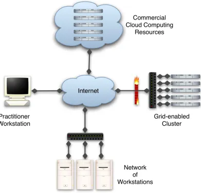
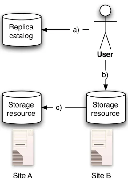
(14) Figure 3.5: Example workflow that only has a single level of iteration..................................77 Figure 3.6: An example workflow which illustrates how exposing inner iterations improves the degree to which a workflow can be executed in parallel................................................... 78 Figure 3.7: Example of an operator declaration for an R script............................................... 78 Figure 3.8: An abstract view of the invocation of an operator. Operators are invoked by the workflow, with operators looked up by name from an operator list and input and output data mapped to their ports............................................................................................................... 80 Figure 3.9: Data source declaration for the Iris flower data set............................................... 81 Figure 3.10: Hierarchy of parallelism from CPU level, to LAN level, up to WAN level........82 Figure 3.11: Components which exist within an agent: agent controller, workflow component and data management component........................................................................................... 83 Figure 3.12: Flow chart of events when invoking an operator, including data preparation and retrieval.................................................................................................................................... 84 Figure 3.13: Sequence diagram of executing a remote task, including the staging of data.....86 Figure 3.14: Data management component provides a service for operator adapters to access local and remote data............................................................................................................... 92 Figure 3.15: Provenance information collected by the operator is stored using the metadata component............................................................................................................................... 98 Figure 3.16: Flow chart of components that are required to schedule a workflow. The workflow is segmented into discrete tasks, and these tasks are scheduled for execution......100 Figure 4.1: Attributes that contribute to scheduling: data, tasks, resources and network link. ............................................................................................................................................... 104 Figure 4.2: In a master-slave system there are a number of specialised queues and scheduling systems that may impact on the performance of an execution..............................................108 Figure 4.3: Process of data migrating from its initial location. First it is copied from the Practitioners Workstation to Resource 1, then from Resource 1 to Resource 2.....................110 Figure 4.4: Compute-first matching heuristic. Matches tasks to the resource which will complete the computational component the quickest............................................................ 112 Figure 4.5: Greedy (MinMin) task mapping heuristic........................................................... 112 Figure 4.6: Sufferage mapping heuristic................................................................................ 113 Figure 4.7: Neglected matching heuristic maps tasks to resource when a resource is near, but not strictly, optimal for the task.............................................................................................. 114 Figure 4.8: Configuration of compute resources connected via a network used in scheduling simulation.............................................................................................................................. 120 Figure 4.9: Workflow used in simulation.............................................................................. 121 Figure 4.10: Component diagram of simulation experiment software.................................. 122 Figure 4.11: CPU Usage Efficiency with increasing CPU dominance (x1)........................... 131 Figure 4.12: CPU Usage Efficiency with increasing CPU dominance (x5).........................132 Figure 4.13: CPU Usage Efficiency with increasing CPU dominance (x10)....................... 132 Figure 4.14: CPU Usage Efficiency with increasing CPU dominance (x100)..................... 132 Figure 4.15: Execution times for varying numbers of parallel arrangements of 20 computational elements, running a data-intensive workflow................................................ 133 Figure 5.1: Frequency of response variables in Hou data set................................................137 Figure 5.2: Workflow for HIA investigation.......................................................................... 146. xiii.

(15) Chapter One 1. Introduction Information Technology (IT) tools have become ubiquitous in modern day science, and are commonly applied as fundamental components of data acquisition and analysis across a broad spectrum of scientific fields. Not surprisingly, IT has also played a seminal role in extending horizons of many scientific endeavours – notably the life and chemical sciences – by providing tools and techniques for exploring data sets that were previously intractable. This has been due primarily to advanced IT techniques that a) enable massive computational power to be applied practically to managing, organising and exploring very large, complex data sets, and also b) vastly increases the capacity of data collection, through devices such as high speed, high resolution, robotic analysis instrumentation, sensor networks, and high resolution telemetry. Similarly large data sets can also be produced through simulation, and calculating or deriving new attributes from previously collected data. For example, in the field of cheminformatics [1], chemical structures are analysed using computer applications that compute chemical, electrical and physical properties of a molecule. data sets generated by the above mechanisms typically result in enormous numbers of records containing many attributes. This phenomenon is often referred to as the data deluge [2] and is also illustrated by the increasing availability of data sets via the internet, and superscience instruments like the high energy physics experiment – the Large Hadron Collider (LHC) – that produce petabytes of data per year. While the characteristic size and complexity of data sets has in part re-defined the potential scope of investigative work, it is evident that increased size and availability of data sets poses special challenges to exploring and revealing their information content. Analysis of large data sets requires the use of specialised techniques, including data mining [3], in order to expose the patterns and structures that relate the response variable to the many 1.

(16) candidate predictor variables. Data mining is particularly important when the system under investigation is not thoroughly understood, and new leads are required to focus future research. However, data mining does not discern between valid and spurious correlations, and may be misled by large numbers of variables. Robust techniques may be applied to begin to overcome these issues, but this requires a large amount of computing time, and still requires a domain expert to validate and interpret the results of the data mining investigation. The project presented in this thesis explores the application of the eScience [4], Grid [5][6][7] and distributed computing [8] paradigms to the fields of computational statistics and data mining. eScience focuses on the use of IT tools within the scientific process while the Grid is a paradigm concerned with the interoperability of distributed computing systems. Data mining and computational statistics have a natural affinity with the concepts of eScience. Particular care must be taken to ensure rigorous record keeping is observed when performing experiments, as in silico experimentation can often be performed so readily that this attention to detail may be overlooked. This has consequences for the repeatability of experiments, and for the recording of novel work that may be further explored at a later date. This study project has produced a framework that allows practitioners to express their data mining process as a workflow – a clear, repeatable plan or sequence of steps for an experiment – which enables the use of Grid computing [9] and Data Grid [10] resources to provide the required computational and data services. To use these resources efficiently and effectively requires an appropriate task scheduling algorithm. Many existing Grid computing frameworks use a task scheduling algorithm based on the greedy MinMin heuristic [11][12], that aims to minimise total computation time by accepting locally optimal solutions at each step. This thesis presents a new scheduling algorithm, Neglected, which is shown to outperform the MinMin heuristic in most situations across a range of typical experiment scenarios. The sections following in this chapter give a brief introduction to eScience, the Grid and data mining, in sufficient detail to appreciate this work, with a more thorough analysis in 2.

(17) Chapter 2.. 1.1. eScience and the Grid The term eScience has been used to describes scientific endeavours that are largely enabled through the use of IT. IT can be employed to provide data management, simulation, instrumentation and/or experiment workflow orchestration. The actual scope and implementation details of these services will vary between implementations, but the essential purpose of eScience is to facilitate discovery which would not be possible without IT enhancements. The Grid is the name of a modern IT paradigm that endeavours to seamlessly integrate researchers, instrumentation, and computing and analysis services on a large scale. The Grid paradigm proposes a small number of standards be used to interface between users, services and other widely distributed components. The purpose of keeping the number of required interfaces low is to improve interoperability and facilitate integration. Distributed identity management for users and services provides authentication and authorisation and is used to tie the Grid components together. This is intended to maximise compatibility and re-usability of the services and components, allowing them to be reconfigured and orchestrated for use in almost arbitrary workflows. Many Grid services build on existing components, such as Grid Computing services, which utilise transitional compute clusters and high performance computers via the Grid mechanism. Similarly, Data Grid services are typically used to expose traditional file systems and databases via standardised Grid interfaces. When discussing the composition of a Grid system, it is important to highlight the roles that humans play. In Unified Modelling Language (UML) [13] terminology they are referred to as actors. In this project several human actors will be discussed. These are: 1. The algorithm developer who designs or implements data processing software; 2. The workflow developer or workflow integrator who develops the workflows which pull together the data sets and the algorithms; and. 3.

(18) 3. The domain practitioner, or practitioner, who will be applying the system provided to analyse their data sets, and also refining the workflows to improve predictive performance. To develop this discussion, consider a scenario in which a workflow integrator actor adapts an existing algorithm for use in data mining in such a way that it can be used within the workflow framework being developed in this thesis. The domain practitioner actor has a number of data sets of interest to their research. The workflow integrator produces a workflow utilising an algorithm, which is run and analysed by the domain practitioner. Once the workflow exists, it is then possible for the domain practitioner to reuse the workflow on other data sets, and possibly tune parameters to optimise their investigations. It should be noted that although there are three distinct roles expressed here, it is not unreasonable to assume some or all of these would be performed by the same physical person, depending on their skill set. The goals of eScience and the Grid are not novel within themselves. Since computers first became available, investigators, integrators and computer scientists have been attempting to use them to perform mundane, repetitive tasks of data collection and analysis. As the speed and capabilities of computers have increased they have been tasked with increasingly complex responsibilities. This also requires the integrators and practitioners to think more about the presentation of the problems for the computers. Simply providing a set of linear instructions to solve a problem does not lend itself to reuse, so more abstract forms of the instructions need to be derived which allow the solution to be used in many situations. In general eScience experiments aim to be easy to repeat and modify, as compared to their physical analogues, so they can be easily copied, modified, repeated and even shared. This means that the process for developing an idea differs from an equivalent physical investigation. With software, it is possible to prototype ideas quickly, and without significant financial penalty, leading to the exploration of many potential lines of investigation. The consequence of this approach is that many pilot investigations can be run, possibly without 4.

(19) due documentation, before the primary or significant investigation is performed. The use of Grid computing for data mining is intended to improve the time-tosolution/completion of a data mining workflow by increasing the number of available processing units available to perform work. By doing this efficiently it also enables larger data sets to be analysed – within the constraints of the data mining algorithm's ability.. 1.2. Data mining Data mining is “the extraction of implicit, previously unknown, and potentially useful information from data”[3]. This is achieved using computer programs – the data mining methods – that implement an algorithm for fitting the data set of interest to an understood structure such as an equation or a decision tree, resulting in a model that represents relationships in the original data set. This model can then be used to better understand the original data set and the system from which the observations were collected, and also used to predict the responses from new, unseen data sets, which has application to decision support systems and other business requirements (Figure 1.1).. Figure 1.1: High level flow chart of the data mining process, and the outputs produced by it. Data analysis in modern scientific investigations are moving towards the use of increasingly larger data sets, containing more observations and larger numbers of attributes. The increase in the number of observations is a consequence of improvements in automated data collection allowing more observations to be collected, and the increasing availability of public data sets which can be combined or integrated to produce a single larger data set. The. 5.

(20) number of attributes collected for each observation is also increasing, once again driven by improved data collection at the instrument, and a growing number of synthetic or derived attributes showing promise or improving predictions. In the field of cheminformatics, where Quantitative Structure-Activity Relationship (QSAR) [14], Quantitative Structure-Property Relationship (QSPR) [15] and Quantitative Structure-Retention Relationships (QSRR) are studied, the data sets are composed of compounds (molecules), and an observed property of the molecule. The attributes of the molecules are calculated from the molecular structure, and can number in the thousands when topological, structural, electrical, solubilities, etc are considered. The analysis of data sets like those just described often requires new, or modified statistical and data mining methods. Traditional statistical methods may not perform well (on their own) when there are a very large number of attributes involved. As an example, a simple method like multiple linear regression (MLR) will not compute an accurate fit when there are large number of attributes as it lacks a robust mechanism for disregarding unimportant attributes. This can be addressed through the use of either a variable selection technique to reduce the attribute space, or by using a more sophisticated linear modelling technique such as partial least squares (PLS)[16]. Obviously PLS is not a novel technique, but this does demonstrate that techniques must be applied within their limits of applicability, which is likely to become a more serious issue when researchers are confronted with increasingly large data sets. In developing new or modified techniques to work on large data sets another issue is the time it takes to execute or “fit” a model. Many robust models have a large time-to-solution. Consider the use case of model validation. 10-fold cross validation, which is the minimum accepted by many practitioners in the field, will escalate the execution time by approximately a factor of 10 due to the 10 repetitions of the process. On a small data set this increase in time-to-solution will not be significant, but the addition of new observations or attributes to the data set will increase the significance of this impact until it becomes an 6.

(21) important consideration. While in some situations it may be acceptable to wait for extended periods for results to be returned, it is often desirable to reduce the time-to-solution as much as possible. It is also desirable to have a strategy for scaling the techniques should future data sets become larger. In this thesis tools will be developed to reduce this time-to-solution.. 1.3. Scheduling Distributed Computing Execution Data mining workflows take one or more data sets as inputs, and apply transformations or operations to these inputs to produce outputs. Within the workflow data will pass from the primary sources of data, through the operators and finally to the data sinks. Depending on the type and size of the data, considerations about data location may affect the time-to-solution just as significantly as the number of computational elements, or their speeds. There are two components to the transfer time problem, 1) the network speed, and 2) the network latency. Network speed is significant for large data transfers, and ultimately limits the transfer time. Network latency - the amount of time it takes signals to travel between hosts - is significant for small data transfers as it begins to dominate the actual transfer time when the data occupies only a few packets. This penalty for transferring data is the typical motivation for performing coarse grained parallelism in distributed environments, and restricting fine grained parallelism to clusters and shared memory machines. In the general case the workflow scheduler should be able to place the tasks appropriately to minimise time to completion by taking into account processing speed and data transfer speed. By modelling the workflow in finer detail it becomes possible to effectively have the workflow system adjust the coarseness of the parallelism by scheduling tightly coupled sections on low latency sections of the network. This has particular applicability in scenarios where there is a mixture of single CPU and multiple CPUs per machine, as the workflow can be decomposed to an extent where the CPUs are being used efficiently on a specific section of workflow which would have otherwise required large data transfers.. 7.

(22) 1.4. Project Summary The project described in this thesis had the goal of designing and prototyping an eScience system to address the requirements of data mining practitioners. This involved the collection of requirements based on first hand data mining experience, a survey of existing tools used by data mining practitioners in their work, and then the design and implementation of a prototype system to demonstrate the utility of such a system. This involved developing a simple workflow language which could elegantly capture the experiments data mining practitioners typically execute, and developing a task scheduling algorithm to improve the time-to-solution for executing data mining workflow across distributed hardware.. 1.5. Contributions This thesis makes several contributions to the fields of eScience and data mining. These are summarised as follows: 1. This thesis provides analysis of some typical data mining workflows and develops a general template for these investigations. From this template it is possible to determine the limiting factors in parallelisation, and to enable the understanding of the computational and data requirements for supporting the execution of these investigations. 2. This thesis presents a workflow model which addresses the requirements developed from the general model of data mining, and the design and implementation of a workflow engine to execute this workflow model. 3. This thesis adapts contemporary master-slave scheduling algorithms to efficiently schedule tasks derived from the workflow. Simulation studies have been conducted using the GridSim [17][18] toolkit, investigating the performance of these scheduling algorithms on a number of different network topologies.. 1.6. Thesis Organisation The remainder of this thesis is organised as follows: Chapter 2 presents a detailed 8.

(23) background of the application areas, and the technologies involved. Chapter 3 develops a framework which can be applied to the application areas to achieve the benefits of eScience and the Grid. Chapter 4 formalises the scheduling problem, and presents a new heuristic to address the problem. Chapter 5 presents a study performed using the framework, utilising modern data mining techniques to model the absorption of pharmaceuticals via the human intestinal pathway. Chapter 6 presents conclusions and future work.. 9.

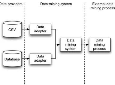
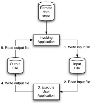
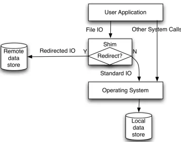
(24) Chapter Two 2. Background and Overview Increases in the volume and resolution of data available for scientific endeavours is a consequence of technological advancements which allow more, higher quality data to be collected more easily. In recent years many large scale projects have provided frameworks for the automatic integration and collection of data from analytical instruments [19][20], sensor networks and large scale scientific projects. These concepts are being enhanced and informed by initiatives such as the OpenData [21] movement, which aims to standardise data formats, and encourage free and uninhibited access to data collected by researchers, in particular involving publicly funded projects. Increases in the production and availability of data sets create a situation termed the data deluge [2]. The ability of researches to use this data will be dependent on the availability of tools to discover and robustly analyse it. eScience aims to provide these tools, and in this chapter the requirements around data mining will be evaluated in an eScience context. This chapter continues the discussion of the large and complex scientific data sets from Chapter 1, and covers the use case of data mining and computational statistics discussing their adaptation into an eScience framework. Initially, the field of cheminformatics is introduced as an example of a field where the growing size of data sets offers opportunities to improve scientific outcomes. Then the requirement for the use of computationally intensive data mining techniques is illustrated with a discussion of cross-validation, metamodels and randomisation techniques. Next, requirements for performing data mining within an eScience context are explored, including the use of a workflow to express the data mining process. Following this, a summary of distributed computing practises is presented, which identifies candidate resources, and approaches to utilising them. And finally, this chapter presents an overview of projects which have previously contributed towards the requirements identified for this project. 10.

(25) 2.1. Robust Data Mining of Large Data sets As outlined in Chapter 1.2, data sets are increasing in size and complexity, requiring new methods and approaches for their analysis. There exist many contemporary data mining methods that can be applied to these large data sets, however, these methods often have long execution times. However, many methods, and other processes of data mining fall into a class of problem that is naturally suitable for distributed computing. In addition, concepts and processes within data mining experiments can be readily mapped to eScience concepts, allowing a natural adaptation of common data mining tasks to an eScience and distributed computing framework. This approach will be covered in detail in the following sections. Data mining is performed through the application of computational techniques to produce predictive and explanatory models of an observed system. Data mining typically uses standard types of models, such as decision trees and linear equations, and fits parameters and structures of the model to the observations. There are many different data mining techniques which take different approaches to the fitting process. Some techniques produce models which are better for explanation than prediction and vice versa. These techniques were developed and used in a variety of disciplines including statistics, computer science, artificial intelligence and machine learning. Data mining techniques have applications that reach far beyond the disciplines that contributed them. In general, data mining can be applied to most fields which collect quantitative data, and is typically applied when there is no existing model of the system under investigation. The application to a new problem area requires different models and fitting techniques to be evaluated to determine the properties of the data, and the suitability of the particular model for that data. Robust data mining refers to data mining techniques that are able to handle either large data sets, or high dimensional data sets without negative impacts such as: •. Over fitting – when a model is too closely matched to the input data that it is unable to perform on new unseen data, and 11.

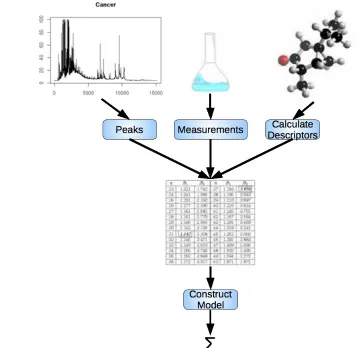
(26) •. The influence of outliers – an observation “... that appears to deviate markedly from other members of the sample in which it occurs.”[22], which can skew the data.. The remainder of this section will introduce cheminformatics, being the application area considered in this thesis, introduce the data mining process in the context of eScience, discuss the options for improving the execution speed of an experiment, and will then analyse some contemporary data mining techniques and experiments. This will results in a set of requirements being developed that encompasses what is to be achieved by this project.. 2.1.1.. Cheminformatics – Data mining in Chemistry. In this thesis the application area of cheminformatics [1] will be discussed and used in examples. Cheminformatics is the application of data mining techniques to the prediction and understanding of chemical systems. The particular field of cheminformatics discussed here is Quantitative Structural Activity Relationships (QSAR) [14], which relates some measure of chemical activity (response) to the chemical properties (predictors). A typical pharmacological application of QSAR would be to relate the bio-availability or absorption of a drug to the chemical structure of that drug. Predictors for cheminformatics include measured molecular properties such as the near infrared (NIR) and mass spectrometry (MS) spectra, measured physical properties such as melting point, and other calculated properties known as molecular descriptors which are derived from the 3D molecular model of the compound (Figure 2.1). There also exist specialised data mining techniques which can utilise the 3D models directly, but in this thesis the focus will be on the use of numerical data sets. All of the numerical data sets indicated here have the property of having a very large number of predictors. In the case of NIR or MS data sets there may be 10,000 or more ordered points and can be gigabytes in size, while descriptor data sets may have over 1,000 molecular descriptors. The significance of having so many predictors must be considered in the context of a pharmacological experiment which may have only a few hundred observations, meaning that spurious correlations. 12.

(27) between the predictor and response become likely. In order to handle this, either a variable selection pre-processing step needs to be applied to reduce the number of predictors, or a robust technique which works well in high-dimensional space should be applied. Both of these options typically have significant execution times Both of these approaches will be discussed in more detail in the next section.. Figure 2.1: Process of distilling various sources of chemical observations into a table of data, from which a model can be built.. 2.1.2.. Data Mining as eScience. From the inception of many scientific investigations, information technology plays an integral role, beginning with experiment design and preliminary calculations, through to the laboratory reports and field trips where the data are collected. Direct data entry or data capture is being used to improve the quality and handle the quantity of measurements and observations, replacing situations where hand written tables would be used. Direct data. 13.

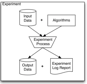
(28) collection means that data can be curated or stored immediately along with experimental metadata associated with the data sets. Storing and organising the experimental data as it is generated gives the opportunity for data processing to begin while the remainder of the experiment is completed. This data can be used as quality control for the experiment, and to assist in tuning or optimising the experimental apparatus in the lead up to the main data collection stage of the experiment. As described in Section 1.1, eScience is a term used to describe scientific endeavours that utilise information technology as an integral part of the process of scientific investigation. Exemplar eScience projects include Comb-e-chem [20] in chemistry, myGrid [23][24] in bioinformatics, and GEODISE [25] in engineering. Key themes in each of these projects include data and provenance management, experiment management via workflows, and distributed execution of tasks. Further, these projects, and others, strive to present this functionality as flexible services – middleware – that can be reused in other projects. As well, the required use of abstract experiment representations – workflows – ensures that the experiments being carried out are guaranteed to have at least a minimum level of standard documentation, aiding in the repeatability of the experiment and the integrity of the results. It is proposed here that this holistic application of object oriented design, service oriented architectures, and the general desire for interoperability and reuse of components is critical in discriminating eScience from science simply done with computers. Often existing middleware providers are utilised, such as Grid computing, as the provider of computational resources. A data mining experiment is a process that applies operations or transformations to input data to produce output data, models, and experiment reports (Figure 2.2). In eScience the experiment process is referred to as the workflow, and the experiment reports are the provenance and metadata of the experiment. eScience commonly relates to input and output data in the same way as data mining.. 14.

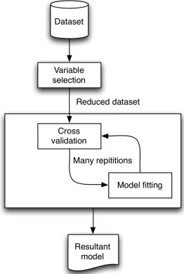
(29) Figure 2.2: An experiment is the application of a process on input data and algorithms, to produce output data and an experiment log. The model for a data mining process that will be considered in this thesis involves three distinct concepts: variable selection, cross-validation, and model fitting (Figure 2.3). Variable selection is a data set reduction technique that can improve runtime and predictive performance of data mining methods by removing clearly redundant variables from the data set; model fitting is the application of the data mining method; and cross-validation is an iterative technique for evaluating the real-world performance of a data mining method. The process of eScience closely emulates the world of physical science. It involves data management, experiment management, workflow enabled data processing, as well as parallel and distributed computing. eScience sometimes enables physical science, while at other times eScience is itself an end, with experimentation occurring via simulation producing quantities of data which subsequently require analysis. In this thesis the entire data mining process is considered in the context of the eScience paradigm, with the intention to exploit eScience experiment and process management approaches, and to achieve an efficient speedup through parallel execution. In fact, it can be seen that the data mining process, when 15.

(30) presented in this way, is a very close match to eScience ideas.. Figure 2.3: Typical data mining process considered in this thesis. To achieve the outcomes of parallel data mining execution requires a data analysis system designed to support this functionality, but the benefits of faster execution time are significant. Whether the analysis is being performed for real-time applications, or the system is being used for the development of analysis techniques, reducing completion times from days to hours, or hours to minutes can be of significant value.. 2.1.3.. Efficiently Speeding Up Execution. The most effective method for improving the execution time of an application depends on many factors, such as: the language used to implement the application, the algorithms and 16.

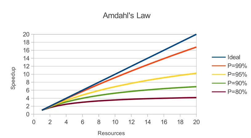
(31) design of the application, and the way it uses data. Applications which are implemented using scripting languages can often achieve speedups by re-implementing (at least the slow method) in a compiled language, as this removes the interpreter and type checking overhead. Many scripting languages provide efficient ways to achieve common tasks, such as R[26], where you can achieve upwards of a 10 times speedup for loops if you use the apply method instead of a for loop. Another approach to achieve speedup is to ensure the data are stored in an efficient way in memory, so that processing it does not incur unnecessary operations to transform it. For instance, the use of strongly typed, primitive arrays are much faster to access than object arrays. This is due to a couple of reasons: firstly the primitives are normally a smaller data type, so will fit better in memory and cache memory; and secondly because objects will normally be converted to primitives for the CPU to process, and this conversion incurs an overhead. Once it is clear that the application is as efficient as is practical, it is possible to consider using multiple computing resources to perform the work. Parallel processing adds an extra level of complexity to the application, as it will now have to consider coordinating these resources, transferring data if required, and recombining the output data. This added complexity and overhead can make it impractical for smaller applications, but once the framework is established, it is possible to continue to scale to additional resources.. 17.

(32) Speedup. Amdahl's Law 20 18 16 14 12 10 8 6 4 2 0. Ideal P=99% P=95% P=90% P=80%. 0. 2. 4. 6. 8. 10. 12. 14. 16. 18. 20. Resources. Figure 2.4: Amdahl's law showing the speedup obtained by adding additional resources. The benefit gained by adding additional resources to an application is described by Amdahl's law, which expresses the diminishing returns of adding additional resources as a function of the percentage of the application that can be made parallel (Figure 2.4). This is expressed as:. Speedup=. 1. (2.1). P ((1−P)+ ) S. Where S = the number of resources, and P is the percentage of the application that can be made parallel. To be made parallel in an efficient way the application needs to be broken into tasks that have minimal data communications overhead, ideally only requiring communications at the start and end of the execution (loosely coupled), and where the execution time dominates the communication time (coarse grained). Applications that can be broken into coarse grained, loosely coupled tasks are in the wellknown class of parallel programs called embarrassingly parallel (EP) [27]. EP problems can be efficiently solved using up to n independent machines, where n is the number of models. Consider a single task that occurs in three distinct steps:. 18.

(33) 1. Load data into memory, 2. Compute model, and 3. Return result. The time taken to perform steps 1 and 3 will be limited by the bandwidth and latency of the connection between the main memory of the machine and the storage resource being used to store the data. When the data are local to the machine it may be much faster than if the data are stored on a remote machine accessed via a network. For an EP problem the time taken to perform step 2 will be limited by the speed of the CPU in the machine. There also exists a spectrum of parallel applications which require data to be transferred between tasks during execution, and are described by the frequency with which these exchanges occur, from coarse grained to tightly coupled. In this spectrum of parallel applications the time taken to perform step 2 will also be affected by the latency and bandwidth between machines, in addition to the CPU speeds of the other machines and their own CPU speeds. This is because resources have to wait while other CPUs calculate and deliver the data they depend on, resulting in idle CPU time. From this discussion it should be clear that efficient parallel processing is dependent on being able to break the data mining application into coarse grained, loosely coupled tasks. The discussion of parallel processing will be continued in Section 2.4. Next, contemporary data mining techniques will be introduced, and assessed as to how they can be efficiently parallel processed.. 2.1.4.. Review of Contemporary Data Mining Techniques. There are a large number of data mining algorithms and techniques employed in a field like cheminformatics. They include classification, regression and clustering techniques, and aim to produce both predictive and explanatory models to aid the practitioner in their work. The effectiveness of a technique will be influenced by the data, and the desired outcomes of the practitioner. Data dimensionality will be a primary driver in the selection of the. 19.

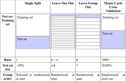
(34) algorithm, with many methods failing as the number of variables increases, requiring variable selection as a pre-processor. Many methods can only utilise either continuous or categorical data, and may not be able to handle missing values. Depending on the form of the model, there will be a trade-off between a complex model which has a high degree of predictive power, but is hard to interpret, and a simpler model which has less predictive power but is more easily used as an explanatory model. Once a model has been fitted to a data set it is important to know how well the model represents the data. There are a number of methods which compare the predicted and actual responses. Two very commonly reported figures are error and variance. These are commonly reported as mean absolute error, MAE, often calculated as a mean squared error, MSE, or its square root, RMSE, which all approach zero as the model improves. Variance can be calculated using Pearsons correlation coefficient, r, or it's square R2 which approach 1 as the model improves. These methods are covered in more detail in [28] and [29]. However, an important concept to understand when fitting complex, or even some simple models, is that the model needs to be generalised (not over-fit) if it is to be of any use. That is, it needs to be able to make accurate predictions from data that was not in the original data set. Evaluation of this requires that an external test set be available to validate the performance of the model. This process is known as cross validation (CV). There are a number of specific approaches to cross validation summarised in Table 2.1. The selection of a CV technique will depend on the type of data, the size of the data set, and the requirements for time-to-completion and the accuracy of performance metrics. Simply splitting the original data set into a test set and a training set is straight forward and computationally inexpensive, but it does not robustly evaluate the performance as artefacts in the test or training set can give misleading results. Leave One Out (LOO) validation iteratively selects each observation from the data set and removes it as the test set, performing the model building process on the remainder of the data, and averaging the resultant figures. Due to the small size of the test set this method is also prone to issues such 20.

(35) as high variance [30][31], and it comes at a higher computational cost. A variation on the LOO is leave group out (or k-fold), where a fixed number of observations are removed into the test set. This number is typically N/k where N is the total number of observations and k is the number of times this will need to be repeated to use all observations in a test set. This offers better computational performance than LOO, and can also avoid the high variance drawbacks. Leave one out is a special case of leave group out, where k=N. Monte-carlo cross validation (MCCV) [32] is a more robust and accurate performance estimation technique, which approaches the performance estimation problem as a montecarlo simulation. At each iteration of the validation the data set is split, with training and testing performed as before. However, this process is repeated hundreds or thousands of times, and an aggregate of the measured performances is reported as the result, meaning it is computationally the most expensive. This process eliminates any bias which may accidentally occur due to the prior ordering of the data, but does so at great computational expense. To appreciate the impact of the computational expense of each cross-validation technique, remember that each training iteration involves performing the model fitting, which itself may be a computationally expensive operation. For example, if a data mining technique takes 1 minute to fit the model on 100 observations, it will take ~1 minute to cross validate under a single split CV, 10 minutes under 10-fold CV, 100 minutes under LOO CV, and 1000 minutes under MCCV.. 21.

(36) Single Split. Leave One Out. Leave Group Out. Test set- Training set Training set. Monte Carlo Cross Validation Training set. Test set Test set. Runs. 1. Test set ~30% size Group order. k=n. k. 1000+. n/k. 1. 50.00%. Selected or randomised Randomised at start start. at Randomised start. at Randomised each run. at. Table 2.1: Summary of cross-validation technique procedures, relating number of iterations required to n=observations and k=testsets. Data mining aims to fit a general purpose model to a data set through a calibration process. General purpose models are used because the exact physical mechanisms of the system under observation may not be fully understood. It is not expected that an exact fit will be achieved as general purpose models are being used, and accordingly there is a large and increasing number of data mining methods available to fit models catering for various types of data. Some typical models include decision trees, linear or non-linear equations and metamodels. While some sophisticated methods are able to robustly fit the training data, there is also a class of meta-models which can utilise simple, weak learners, such as decision trees with a single split, or linear regressions built with a small number of terms. When many models are combined together like this they are referred to as ensemble methods. Most of these metamethods heavily utilise randomisation in the generation of the individual models as a mechanism to avoid bias. Ensembles(Figure 2.5) are one class of meta-method that may employ randomisation. 22.

(37) when combining their base learners. An example of this is bootstrap aggregation or bagging [33] (Figure 2.6), which trains many models on a sample (bootstrap) of the training set. The bootstrap sample is of the same size as the original training set, and is sampled with replacement, meaning that some observations will appear many times. When evaluating the bagged model all the individual models are evaluated, and the average of the predictions is used. The resultant model has a low variance and is more resilient to overfitting. Another example of an ensemble is boosting, which takes a base learning method and produces many individual models using subsets of the input data variables, and combine these individual models into a single larger model.. Figure 2.5: Generic ensemble of independent weighted models.. Figure 2.6: Bagging: Ensemble of independent weighted models built on subsets of the data.. One popular ensemble technique which utilises bagging is Random Forests [34]. Random Forests uses decision trees as the weak learner. Each tree is trained on a bootstrap of the training data, and at each node a bootstrap of the predictors is used to calculate the split. This is repeated for a number of trees which are combined to make the Random Forest ensemble. Random Forests can perform well in the presence of many predictors, and produces accurate predictions in many situations. Another popular data mining technique for cheminformatics is the Support Vector Machine (SVM) [35]. SVMs can be used for classification and regression and offer a robust approach to fitting models. Importantly, they can be used with various kernel transformations 23.

(38) on the input data which allows them to fit non-linear data sets.. 2.1.5.. Typical Data Mining Experiments. In this section the development cycles of two actors are discussed: data miners who are interested in analysing data sets; and algorithm developers who are interested in producing and evaluating new data mining techniques. Both these groups have the same core requirements, although they approach the problem from different angles. First the data miner's environment will be described, and then the algorithm developer's environment, highlighting the differences. Data mining practitioners start their work by identifying a data set of interest. Whether they collect the data themselves or derive it from other data sets is not relevant, but in either case it is assumed they can identify the response and predictor variables so these can be considered as generic data sets. Assuming the data are in an unprocessed form it will now be analysed to test the quality of the data set, filtering out homogenous variables, and perhaps centring and normalising the variables. Next a decision will be made by the practitioner about the validation technique that will be used. All validation techniques involve splitting the data set into two parts, training a model on one part, and evaluating the model's predictive capabilities on the remaining part (Figure 2.7), and each research field that utilises data mining tends to have its own accepted validation technique. Following this, the actual modelling techniques to be used on the data must be selected. This decision will be guided by a combination of domain knowledge, the linearity or nonlinearity of the data, whether the model is for prediction or understanding the data, and personal preference and experience. Nearly all but the simplest of modelling techniques will require a number of parameters to be set, requiring manual selection by rules, automatic tuning algorithms, or parameter sweep operations.. 24.

(39) Figure 2.7: Flow chart of cross-validation as applied in data mining. 25.

(40) Finally the practitioner will execute the experiment with the selected validation, model, and parameter selection, and will analyse its performance. This may lead to changes in the set up, and re-running of the experiment in an attempt to improve the outcome. Ultimately the experiments will produce a model which the practitioner can use to predict new unseen data, or be used to describe the system from which the data was originally collected. Data mining practitioners will hold the data set and probably the model constant, and attempt to tune the parameters to get the best performance from the models and the best understanding of the system. Algorithm developers are typically interested in using many data sets, selected for their data type or origin (spectral, QSAR, etc) and using these to evaluate the algorithm or modelling technique they have developed. Therefore algorithm developers will hold the model and possibly the parameter selection constant, and evaluate across many data sets. An example of this kind of experiment is presented in Appendix A.. a). b). 1. 2. 3. 4. 5. 6.. clean data cross validation variable selection model parameter selection model building summarise. 1. 2. 3. 4. 5.. data sets clean data cross validation model building summarise. Figure 2.8: Abstract representation of the list of steps for the generalised process that a) data mining practitioners and b) algorithm developers, may use in their work. Figure 2.8 shows an abstract list of steps that a data mining practitioner and algorithm developer may use in their work. Indentation represents sub-steps that are performed in the context of the higher level indentation. In both cases, each iteration of the cross validation will require a model to be built. It is clear that there are common constructs between these two lists of steps. The common structures of these lists are extracted and presented in Figure 2.9 as a generic template that demonstrates these structures. It is not intended to be fully representative of the work practices of of all data mining practitioners, but rather it capture. 26.

No results found