This is a repository copy of
Intergenerational analysis of social interaction
.
White Rose Research Online URL for this paper:
http://eprints.whiterose.ac.uk/43081/
Monograph:
Brown, S., McHardy, J. and Taylor, K. (2011) Intergenerational analysis of social
interaction. Working Paper. Department of Economics, University of Sheffield ISSN
1749-8368
Sheffield Economic Research Paper Series 2011007
[email protected] https://eprints.whiterose.ac.uk/
Reuse
Unless indicated otherwise, fulltext items are protected by copyright with all rights reserved. The copyright exception in section 29 of the Copyright, Designs and Patents Act 1988 allows the making of a single copy solely for the purpose of non-commercial research or private study within the limits of fair dealing. The publisher or other rights-holder may allow further reproduction and re-use of this version - refer to the White Rose Research Online record for this item. Where records identify the publisher as the copyright holder, users can verify any specific terms of use on the publisher’s website.
Takedown
If you consider content in White Rose Research Online to be in breach of UK law, please notify us by
Sheffield Economic Research Paper Series
SERP Number: 2011007
ISSN 1749-8368
Sarah Brown, Jolian McHardy and Karl Taylor
Intergenerational Analysis of Social Interaction
March 2011
Department of Economics University of Sheffield 9 Mappin Street Sheffield S1 4DT
United Kingdom
Intergenerational Analysis of Social Interaction
∗Sarah Brown, Jolian McHardy and Karl Taylor
Department of Economics, University of Sheffield,
9 Mappin Street, Sheffield, United Kingdom,
S1 4DT.
Abstract
We explore the relationship between the social interaction of parents and their offspring from a theoretical and an empirical perspective. Our theoretical frame-work establishes possible explanations for the intergenerational transfer of social interaction whereby the social interaction of the parent may influence that of their offspring and vice versa. The empirical evidence, based on four data sets covering Great Britain and the U.S., is supportive of our theoretical priors. We find robust evidence of intergenerational links between the social interaction of parents and their offspring supporting the existence of positive bi-directional intergenerational effects in social interaction.
Keywords: Social Interaction; Intergenerational Transfer JEL Classification: D19; H24; H41; H31
∗We are grateful to the Data Archive at the University of Essex for supplying the National Child
1
Introduction
Over the last two decades there has been increasing interest in the economics literature in the implications of social interaction and social capital for socio-economic outcomes such as educational attainment and employment. Given that social skills, and personal-ity characteristics in general, are an important part of human capital, see Bowleset al. (2001), it is not surprising that the relationship between social interaction and socio-economic outcomes such as education has attracted growing interest in the socio-economics literature. In general, empirical evidence supports a positive relationship between social interaction and educational attainment, see, for example, Brown and Taylor (2007), Ian-naccone (1998), and Sacerdote and Glaeser (2001). Furthermore, Glaeser et al.(2002), who report evidence supporting a positive correlation between education and social in-teraction proxied by membership in organizations, state that this relationship is not only well known in the social capital literature, but is also “one of the most robust empirical regularities in the social capital literature.” (Glaeseret al., 2002, p. F455).
It is apparent that intergenerational aspects to the accumulation of social capital may exist as in the case of human capital accumulation. A vast literature exists exploring the determinants and implications of human capital, with recent interest in intergenera-tional aspects such as the link between the human capital of parents and their children. A number of explanations have been put forward to explain the existence of a positive intergenerational relationship in educational attainment. Firstly, it could be due to ge-netic transmission of ability, i.e. more able parents have more able children. Secondly, it could reflect a direct transfer of knowledge from parent to child, whereby parents with higher levels of education are more able to help their children with their learning. Alternatively, it may be due to economic factors such as income and wealth, with such resources providing access to, for example, books and private tutoring. In practice, however, it is likely that a combination of these factors is responsible for the observed positive relationship between parents’ and children’s human capital (see, for example, Cunha and Heckman, 2007; Blandenet al., 2007).
In contrast to the human capital literature, the relationship between parents’ and children’s social interaction is relatively unexplored in the economics literature. One might conjecture that if a child is brought up by parents who are socially active, then this may become the norm for the child. Indeed, in the context of the more general concept of social capital, Putnam (2000) remarks that “the parents’ social capital ... confers benefits on their offspring, just as children benefit from their parents’ financial and human capital,” (Putnam, 2000, p. 299). Similarly, Brown and Taylor (2009) argue that an intergenerational link between social interaction may exist whereby parental so-cial interaction may be positively associated with their children’s involvement in formal social activity, which in turn may be conducive to human capital accumulation.
re-sources; parenting practices; genetic inheritance, and role modelling, whereby the latter two explanations find relatively more support. In a similar vein, Vesel (2006) explores whether social capital is transmitted from parents to children using survey data relating to the Czech Republic. The empirical analysis, which is based on establishing correla-tions rather than causal relacorrela-tionships, suggests weak intergenerational transmission of social capital. Similar findings are reported by Jennings and Stoker (2004) relating to the intergenerational transmission of social trust. In contrast, Beck and Jennings (1982) report a strong correlation between parents’ and children’s civic participation in the U.S.
In the economics literature, Guiso et al. (2008) model the intergenerational trans-mission of priors about the trustworthiness of others within an overlapping generations framework. Following Dohmen et al. (2007), using the German Socio-Economic Panel (GSOEP), they report empirical evidence supporting a positive correlation between the trust of parents and their children by modeling the effect of parents’ trust on their chil-dren’s trust. Due to the limited availability of information on the key variables such as trust, which were elicited from parents and all their offspring who were aged 18 or over at the time of the interview, these two studies analyse information mainly drawn from the 2003 and 2004 waves of the GSOEP, and hence they are unfortunately unable to exploit the panel nature of the data.
More recently, within the economics literature, using data drawn from the U.S. Na-tional Longitudinal Survey of Youth 1979, Okumura and Usui (2010) explore the effect of parents’ social skills on their children’s sociability. Respondents aged between 20 and 28 were asked about their sociability as a child such as the number of clubs they participated in during high school, whereas, due to the absence of information on their parent’s social skills, parent’s social skills are proxied by the people skills needed in the occupations the respondent’s parents were in when the respondent was aged 14.1 Support is found for a positive association between children’s sociability and the proxy for parents’ social skills.
In this paper, we focus on social interaction rather than the arguably more general concepts of social capital and trust. Moreover, although a small number of existing studies in this area have presented interesting empirical evidence supporting the exis-tence of positive correlations between the social capital of parents and their offspring, it is apparent however that inferences relating to causality cannot be drawn from such studies. In addition, existing studies have not allowed for the possibility that a parent’s social capital may influence that of their child and that the child’s social capital may influence that of their parent. In the context of social interaction, such a possibility is arguably particularly apparent. For example, if a child engages in a range of activities, such as sport or dancing lessons, it is conceivable that parents will become involved in social events associated with such activities or, alternatively, may simply meet other parents which may lead to social interaction or information about social interaction op-portunities. Hence, an important contribution of our paper lies in the fact that we allow for causality to operate in both directions. In addition, we exploit the panel nature of
1
our data in order to shed some light on the causal nature of such relationships. To be specific, our theoretical framework presented in Section 2 establishes possible theoretical explanations for the two-way intergenerational transfer of social interaction. We then explore this intergenerational relationship from an empirical perspective. In order to explore the robustness of our results, our empirical analysis draws on four data sets namely, the British National Child Development Study, the British Cohort Study, the U.S. Panel Study of Income Dynamics and the U.S. National Longitudinal Survey of Youth. Our empirical analysis supports the existence of positive relationships between parents’ and children’s social interaction.
2
Theoretical Framework
In this section we set out a theoretical framework establishing possible explanations for the intergenerational transfer of social interaction, which in contrast to the existing literature, is a two-way process (incorporating movements from the younger to older generation as well as the reverse). The section has two parts. The first part briefly introduces Becker’s (1974) theory of social interaction. The second part extends the theory to explain how two-way intergenerational social capital transfers might arise.
2.1 A Model of Social Interaction
The foundation for our theoretical framework is the model of social interaction developed by Becker (1974). This model incorporates social interaction (as discussed in the broader context of wants and their determinants in, for example, Bentham, 1789; Marshall, 1962) in a framework of household behavior by introducing non-household individuals whose characteristics affect the production of the household’s commodities and which can be influenced by the actions of the household.
Individualihas a utility function
Ui =Ui(Zi1, ..., Ziq), (1)
where Zij (j = 1, ..., q) are commodities (or wants) consumed by individual i. Each commodityZij has a production function
Zij =Zij(xij, tij, ei, Rij1, ..., Rijr), (2)
wherexij and tij are, respectively, the individual’s endowment of market goods or ser-vices and time devoted to the production of commodityj, ei is a measure of the indi-vidual’s education, experience and other relevant personal and environmental charac-teristics, andRijm (m= 1, ..., r) are characteristics ofr ‘other’ individuals that impact uponi’s output of commodityj.
Becker’s (1974) model accordingly in order to provide a theoretical explanation for two-way intergenerational transfer of social interaction.
2.2 Intergenerational Transfers of Social Interaction
Like Becker (1974) we begin with a simplified situation in which there is a single com-modity, Z. However, in terms of factors which affect Z we include the characteristics of the household’s children in addition to the characteristics of ‘other’ individuals. Es-sentially, we employ a model in which the household, composed of parents and one or more children, is separated according to (i) income earners and decisions makers (par-ents) and (ii) non income earners and non decision makers (children). We distinguish between the parents and the children with the parents of householdigaining utilityUi according to Eq. (1) and the children entering parents’ utility through the production function Eq. (2) in terms of their characteristics which we denoteRc. For clarity, we now refer to the ‘other’ individuals whose characteristics feature as inputs in i’s production function in Eq. (2), as ‘non-household’ individuals, and denote their characteristicsRn.2
Whereas Becker (1974) includes a single good x as an input into the production of
Z, we include time. Let:
T =Tw+Tc+Tn, (3)
whereTs (s=c, n) is the time required in the production ofRs,Tw is the time devoted to work and T is the total available time. An important assumption in our argument is that Ts incorporates not only time devoted to producing Rs, it also includes time involved in searching for Rs prospects: hence, we envisage a scenario in which there is imperfect information over the available production opportunities and so our model involves search costs.
Maximising utility is now equivalent to maximising the output of commodityZ based upon the utility-output function:
U =Z(R, T), (4)
where R is a two-vector. Following Becker (1974), we assume that the characteristics
Rc and Rn have two components:3
Rs=Rs(Ds, hs), (s=c, n), (5)
wherehsis the effect of the parents’ effort on the characteristics ofsandDsis the level of Rs when the parents make no effort. We assume that Rs is increasing in both its arguments:
∂Rs
∂gs
>0, (g=D, h). (6)
Furthermore, we are interested in introducing into the ‘non-household’ characteristics,
Rn, the characteristics of the household’s children. The argument is that the attitude of non-household individuals towards the parents,Rn, is improving in the level of household investment in children’s characteristics reflecting, for instance, the social pressure on
2
We drop theiandjsubscripts henceforth as the meaning should be clear from the context.
3
being seen to be giving children positive social experiences. To reflect this Eq. (5) becomes:
Rc =Rc(Dc, hc), (7a)
Rn=Rn(Dn(hc), hn), (7b) whereDn is increasing and concave in its argument:
D′
n(hc)>0, Dn′′(hc)<0. (8) Hence, parental investment in child social interaction, hc, has a direct positive effect on child characteristics, Rc, and a further indirect positive effect on ‘non-household’ individuals’ characteristics,Rn.
Eqs. (7a) and (7b) require some explanation in the context of the themes of this paper. Parents can invest in ‘non-household’ characteristics by raising their own so-cial interaction level, hn, for example, by increasing their club membership, level of volunteering and so on. They can also invest in ‘child’ characteristics by raising their children’s social interaction, for example, by enrolling their children in more clubs and activities. However, child and non-household characteristics have an autonomous part,
Ds (s=c, n): in the absence of any investment ‘child’ and ‘non-household’ characteris-tics may be non-zero. (Of course,Ds can be negative: before any investment inhs the ‘social environment’ is negative.) In the case of ‘non-household’ characteristics the term
Dn is quasi-autonomous as it is only constant given changes in hn but, by Eq. (8), is increasing inhc.
It follows from Eqs. (7a) and (7b) that maximising utility, Eq. (4), can now be meaningfully expressed in terms of the arguments hn and hc (since Dc is exogenous) which we represent by the two-vector,h:4
U =U(h). (11)
It is now clear that the input of timeTs required in the production ofRs (s=c, n) can also be specified in terms ofhs, hence Eq. (3) can be written:
Ts=tshs, (s=c, n), (12a)
T =Tw+tchc+tnhn, (12b)
4
It is important to note that the dependence of Rn on hc through Dn(hc) in Eq. (7b) is not inconsistent with Eq. (11) having the usual properties (quasi-concavity in the argumentshc and hn). We illustrate with the following simple example.
Example 1. LetU(h) =hc.[Dn(hc) +hn], i.e. Dc= 0. The Bordered Hessian forU(.)is given by
0 Dn(.) +hcD′n(.) +hn hc Dn(.) +hcD′n(.) +hn 2Dn′(.) +hcD′′n(.) 1
hc 1 0
(9)
Quasi-concavity requires that Eq. (9)is non-negative, hence
[2Dn(.) + 2hn]− {h
2
cD
′′
n(.)} ≥0, (10)
Inspecting Eq. (10), from Eq. (8), {.}<0. A sufficient condition for (10)to hold is then that[.]>0
wherets is the constant time per uniths.5
One reason for including time in the theoretical framework is to allow us to model search costs in the pursuit of social interaction activities. We initially allow two factors to affect search costs. First, we make the argument that parents may have a stock of knowledge, ˜h, about social interaction opportunities which is based upon, say, previous engagement in social interaction which might include the social interaction of the parents before they had children or, indeed, earlier experiences of social interaction with younger siblings. Hence:
Ts=ts(˜h)hs, (s=c, n), (13) wherets is non-increasing and convex in its argument:
t′
s(˜h)≤0, (s=c, n), (14a)
t′′
s(˜h)≥0. (14b) Second, we recognise that the search costs and hence time involved in one period’s (τ) hs investment, hτs, may be influenced by the search experience relating to hs and
h−s (−s 6= s = c, n) investments in the previous period (τ −1): hτs−1 and hτ−−s1. For simplicity, we consider two periods (τ = 0,1), hence:6
t0s=t0s(˜h), (s=c, n), (15a)
t1s =t1s(h0,h˜), (15b) where the properties of Eq. (15a) follow directly from Eqs. (14a) and (14b), and t1s is non-increasing and convex in its arguments:
∂t1s(h0,˜h)
∂k ≤0, (k=h
0
s, h0−s,˜h) (16a)
∂2t1s(h0,h˜)
∂k2 ≥0. (16b)
Hence, in the initial period,τ = 0, time devoted to each unit of h0s investment,t0s, is a function of the original stock of parental social interaction knowledge, ˜h. In the next period, τ = 1, time devoted to each unit of h1s investment is a function of the original stock of parental social interaction knowledge, ˜h, and the level of investment inh0s and
h0−s activities in the previous period (with such investments yielding search cost time-saving benefits in period τ = 1). We would naturally expect the marginal effect of the
5
We assume that the second derivative here is zero for simplicity. Arguably the term could be positive, reflecting the possibility that additional opportunities for social interaction involve higher search costs or are less time efficient (i.e. the most time efficient opportunities are selected first), or negative, reflecting possible time efficiencies or information advantages (reducing search costs) that might result from each extra unit ofhs.
6
h0 elements ont1s to be dependent upon ˜hand vice versa (by Young’s Theorem), in the following way:
∂2t1s(h0,˜h)
∂˜h∂h0 ≤0. (17)
In words, the time-saving effects in terms of reduced search costs forh1s investments due to periodτ = 0 investments are likely to be smaller if the parents have a higher initial stock of social interaction capital, ˜h. At the extreme, if the parents have such a high stock of capital ˜h that they have full information, then all possible gains from h0s in-vestments in terms of revealing time-saving information are eliminated and ∂t1s(h
0
,˜h) ∂h0 =0.
We now have two time constraints, one for each period that we wish to model. Hence Eq. (12b), can be written:
T =t0w+ X s=c,n
t0s(˜h)h0s, (18a)
T =t1w+ X s=c,n
t1s(h0,˜h)h1s. (18b)
In addition to the time constraints, the parents face a budget constraint:
Iτ = X s=c,n
pshτs, (19)
whereI is money income and psis the price of a unit of hs. As is well known, the three constraints, Eqs. (18a), (18b) and (19), can be collapsed into a single constraint for each time period:
M =wT +V = X s=c,n
h
wt0s(˜h) +ps
i
h0s, (20a)
M =wT+V = X s=c,n
h
wt1s(h0,˜h) +ps
i
h1s, (20b)
where w is the time-invariant and constant wage rate, V is time-invariant non-labour income andM is the household’s ‘full income’ which, assuming for simplicity no saving or borrowing, is also time-invariant across the two periods.7
We now make the following simplifying assumptions. First, we assume that the characteristicsRs do not exhibit memory over the two periods (there are no reputation effects: e.g. investments in Rn in period τ = 0 are forgotten by the non-household individuals in period 1), hence:
Dcτ =Dc, (τ = 0,1), (21a)
Dτn=Dn(hτc). (21b) Second, we assume that the search cost benefits forh1sinvestments due toh0investments are not known to the parents, a priori: hence the maximisation problem is separable over the two periods.8 Finally, assuming an interior solution (so that hτ > 0), the maximisation problem can be stated as:
max h0 U(h
0), s.t. M =w X
s=c,n
t0s(˜h)h0s+ X s=c,n
psh0s, (22a)
7
See Becker (1965) for a derivation and discussion of ‘full income’.
8
max h1 U(h
1), s.t. M =w X
s=c,n
t1s(h0,˜h)h1s+ X s=c,n
psh1s. (22b)
Given that the problem is separable over time, the Lagrangian for the maximisation problem facing the parents in periodτ = 0 is then:9
L(h0) =U(h0) +λ0
"
M −w X
s=c,n
t0s(˜h)h0s− X s=c,n
psh0s
#
. (23)
The relevant first order conditions for an equality constrained maximum are then:10
Lh0
s(h
0) =U h0
s(h
0)−λ0hwt0
s(˜h) +ps
i
= 0, (24a)
Lλ0 =M−w
X
s=c,n
t0s(˜h)h0s− X s=c,n
psh0s= 0. (24b)
We now address the issue of intergenerational transfer of social interaction from par-ents to children. First, if the parent’s utility functionU =Z(R, T) places high value on social interaction, this may be genetically or socially transmitted to the child through a high valuation ofhc inRc(Dc, hc) - i.e. the standard approach to intergenerational trans-fer. Second, given Eq. (7b) the parents (decision-makers) can influence non-household characteristics Rn via investments in their own social interaction activities hn and/or investments in child social interactionhc, they have an incentive to makehc investments even if they do not have a large positive impact on the child (i.e. ∂Rc(Dc,hc)
∂hc is positive
but small). Hence, whilst by Eq. (6) we have ruled out the parents making hc invest-ments that impact negatively on child characteristicsRc, this (second) line of reasoning for parent to child intergenerational transfer of social interaction follows either from the parent’s concern about how they themselves are perceived externally (being seen to do the ‘right thing’ for their children) or out of a belief that regardless of how low a value the child places onhc, they (the parents) know what is best and believe that non-household individuals share the same view (e.g. dance lessons might not be the child’s chosen activity but the parents and non-household members believe they are beneficial). In either case, unlike the first argument, hc investments here may not be sustained if the child was the decision-maker. We now exploit the search cost aspect of our model to explain a possible third source of parent to child transfer of social interaction: if the parents have a high initial stock of social interaction capital ˜h this may reduce the search costs associated with child social interaction investment in periodτ = 0, reducing
t0c(˜h), by Eq. (14a), and hence boosting h0c. It is straightforward to show that this will be true if wλ0∂t
0
n(˜h)
∂˜h
h
wt0c(˜h) +pc
i
is not too large relative to wλ0∂t
0
c(˜h)
∂˜h
h
wt0n(˜h) +pn
i
, and hence h0n-related search costs due to an increase in ˜h do not fall too fast relative toh0c-related search costs. To see this, we refer to the first order conditions for period
τ = 0, Eqs. (24a) and (24b). Taking total differentials, forming a Hessian matrix |B|
9
Becker (1974) is specifically concerned with the size and behaviour of social income: the sum of money income and the value of the characteristics of non-household income. Our purpose here is to examine the behaviour of investments inhs (s=c, n), hence it is sufficient to use money income as the relevant term in the constraint rather than social income.
10
and using Cramer’s rule, given|B|>0 for a maximum:
sign
∂h
c
∂˜h
=sign
wλ0∂t
0
c(˜h)
∂˜h Ucn(h
0) −hwt0
c(˜h) +pc
i
wλ0∂t
0
n(˜h)
∂˜h Unn(h
0) −hwt0
n(˜h) +pn
i
wh∂t
0
n(˜h)
∂˜h h 0 n+
∂t0
c(˜h)
∂˜h h 0 c
i
−hwt0n(˜h) +pn
i 0 (25) Expansion of the R.H.S. of Eq. (25) yields:
w ∂t
0 n(˜h)
∂˜h h
0 n+
∂t0c(˜h)
∂h˜ h
0 c
! n
Unn(h0)
h
wt0c(˜h) +pc
i
−Ucn(h0)
h
wt0n(˜h) +pn
io
+hwt0n(˜h) +pn
i (
wλ0∂t
0 n(˜h)
∂˜h
h
wt0c(˜h) +pc
i
−wλ0∂t
0 c(˜h)
∂˜h
h
wt0n(˜h) +pn
i )
,
(26)
where (.) <0 and [.]>0. Eq. (26) is positive as required if wλ0∂t
0
n(˜h)
∂˜h
h
wt0c(˜h) +pc
i
is
not too large relative towλ0∂t
0
c(˜h)
∂˜h
h
wt0n(˜h) +pn
i
.
We now address the issue of intergenerational transfer of social interaction from children to parents. Here we again exploit the search cost argument, but this time relating to periodτ = 1 hn investments. The Lagrangian for the maximisation problem facing the parents in periodτ = 1 is:
L(h1) =U(h1) +λ1
"
M−w X
s=c,n
t1s(h0,˜h)h1s− X s=c,n
psh1s
#
. (27)
The relevant first order conditions for an equality constrained maximum are then:
Lh1
s(h
1) =U h1
s(h
1)−λ1hwt1
s(h0,˜h) +ps
i
= 0, (s=c, n), (28a)
Lλ1 =M−w
X
s=c,n
t1s(h0,˜h)h1s− X s=c,n
psh1s = 0. (28b)
We now argue that child to parent intergenerational social interaction effects arise because parental investment in h0c provides information about parental opportunities for h1n investment reducing the associated search costs, t1n(h0,h˜), by Eq. (16a). It is straightforward to show that this will be true ifwλ1∂t
1
n(h
0
,˜h) ∂h0
c
h
wt1c(h0,˜h) +pc
i
is not too
small relative to wλ1∂t1c(h
0
,˜h) ∂h0
c
h
wt1n(h0,h˜) +pn
i
, and hence h1c-related search costs due to an increase inh0c do not fall too fast relative to h1n-related search costs. To see this, we refer to the first order conditions for period τ = 1, Eqs. (28a) and (28b). Taking total differentials, forming a Hessian matrix|B|and using Cramer’s rule, given|B|>0 for a maximum:
sign
∂h1n ∂h0 c =sign
wλ1∂t1n(h
0
,˜h) ∂h0
c
Unc(h1) −
h
wt1n(h0,˜h) +pn
i
wλ1∂t
1
c(h
0
,˜h) ∂h0
c
Ucc(h1) −
h
wt1c(h0,˜h) +pc
i
wh∂t
1
n(h
0
,h)˜ ∂h0
c
h1n+∂t1c(h
0
,˜h) ∂h0
c
h1ci −hwt1c(h0,˜h) +pc
Expansion of the R.H.S. of Eq. (29) yields:
w ∂t
1 n(h0,˜h)
∂h0 c
h1n+∂t 1 c(h0,˜h)
∂h0 c
h1c
! n
Ucc(h1)
h
wt1n(h0,˜h) +pn
i
−Unc(h1)
h
wt1c(h0,˜h) +pc
io
+hwt1c(h0,˜h) +pc
i (
wλ1∂t
1 c(h0,˜h)
∂h0 c
h
wt1n(h0,˜h) +pn
i
−wλ1∂t
1 n(h0,˜h)
∂h0 c
h
wt1c(h0,˜h) +pc
i )
,
(30) where (.)<0 and [.]>0. Eq. (30) is positive as required ifwλ1∂t1n(h
0
,˜h) ∂h0
c
h
wt1c(h0,˜h) +pc
i
is not too small relative towλ1∂t
1
c(h
0
,h)˜ ∂h0
c
h
wt1n(h0,˜h) +pn
i
.
Given Eq. (17), we conclude that this child to parent transfer of social interaction is more likely to occur if ˜h is small (hence imperfect information keeps the search costs forh0s high, presenting opportunities for heavy reductions in period τ = 1 search costs due to periodτ = 0 social interaction investments) andhc plays a dominant role in the parent’s utility-output function, hence even if the search costs makeh0ninvestments pro-hibitively expensive,h0c investments, though incurring heavy time penalties, are valued too highly not to undertake. This is consistent with the idea that parents with small children may face heavy social pressure, or attach great value, to their children gain-ing social interaction. But then havgain-ing undertaken h0c investments, it is possible that associated information gains help to reduce the search costs to futureh1s investments, completing the argument.
Against this, however, since hc appears in Rn, any increase in hc will reduce, at no additional cost, the level ofhnrequired to achieve a given level ofRn, and this will tend to reduce the level of hn investment.
We conclude that the following channels support parent to child intergenerational social interaction: (i) the parent’s utility function U = Z(R, T) places high value on social interaction and this is genetically or socially transmitted to the child, (ii) parents make social interaction investments for their children to be seen to be doing the ‘right thing’ or based, not on what they intrinsically value for themselves, but what they believe to be ‘right’ for the well-being of their children, and (iii) parents have a high stock of social interaction capital ˜h which reduces the search costs associated with child social interaction investment. On the other hand, child to parent intergenerational social interaction effects arise because parental investment in h0c provides information about parental opportunities forh1n investment reducing the associated search costs.
3
Data and Methodology
born in a particular week in 1970. For the U.S., thePSID is a nationally representative panel of individuals ongoing since 1968 conducted at the Institute for Social Research, University of Michigan with the latest wave being in 2007. Finally, the NLSY is a na-tionally representative survey sponsored by the Bureau of Labor Statistics of the U.S. Department of Labor, which, since 1979, has a panel aspect, focusing on gathering in-formation on individuals between the ages of 14 and 22. The four data sets, which provide a wealth of information relating to family background, are ideally suited to our purposes since in each data set it is possible to link parents to their offspring allowing us to explore whether intergenerational associations exist between the social interaction of parents and their offspring.
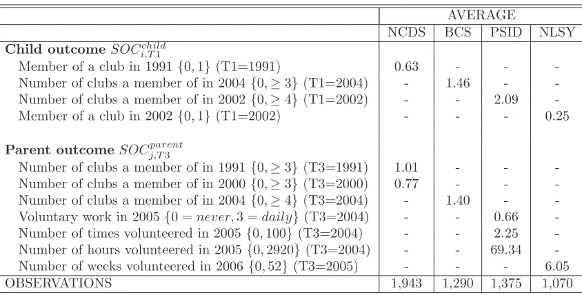
In the NCDS in 1991, when the respondent (i.e. parent) was aged 33, a random sample of one in three of the parents’ children were sampled. Matching parents with their offspring leads to a sample size of 1,943, after missing cases, with the average age of the children being 9 years old. For the BCS in 2004, when the respondents were aged 34, their children were surveyed yielding a sample size of 1,290, after allowing for missing values, with the average age of the children being 12 years old. In the PSID, there is information on the children of the respondents available from theChild Develop-ment Study (CDS) in 1997, 2002 and 2005, which aims to provide information on early human capital formation. In terms of our analysis, we analyse child characteristics in 200211 yielding a matched sample of 1,375 observations, where the average age of the children is 14 years old. Finally, theNLSY allows us to investigate whether any social interaction linkage exists across generations by matching female respondents from the NLSY 1979 with their offspring in 2002, yielding a sample of 1,070 observations, where the average age of the children is 15 years.
In accordance with the small number of related studies in this area as discussed in Section 1, we initially model the social interaction of theithchild (i= 1, .., n),SOCchild, as a function of the social interaction of thejth parent (j = 1, .., m), SOCparent, where the social interaction of both parent and child are measured concurrently, i.e. at time period T1:
SOCi,Tchild1 =X′β
1+γSOCj,Tparent1 +ε1. (31)
We then expand this framework by jointly modelling the social interaction of the ith
child SOCchild and the social interaction of his/her parent as a function of the social interaction of the parent and child, respectively, as follows:
SOCi,Tchild1 =X′β
1+γSOCj,Tparent1 +ε1, (32a)
SOCj,Tparent1 =Z′β
2+φSOCi,Tchild1 +ε2. (32b) Modelling the two outcomes within a bivariate framework allows interdependence be-tween the two equations. Specifically, ε1 and ε2 are the stochastic disturbance terms where ε1, ε2 ∼ N(0,0, σ12, σ22, ρ) and the covariance is given by σ12 = ρσ1σ2. If ρ 6= 0 then joint estimation is characterised by greater efficiency. Finally, the extent of inter-dependence between the social interaction of parents and their offspring is captured by the estimated parametersγ and φ.
11
A major advantage of the data that we employ is that it is generally possible to take account of the fact that individuals are followed over time to allow timing differences in the measures of social interaction. In the empirical analysis that follows we focus on the following approach:
SOCi,Tchild1 =X′β
1+γSOCj,Tparent2 +ε1, (33a)
SOCj,Tparent3 =Z′β
2+φSOCi,Tchild4 +ε2. (33b) whereT1> T2 andT3> T4. This approach reduces the potential for reverse causality since, as argued by Angrist and Pischke (2009), the social interaction of the child (par-ent) is measuredex ante, that is, it predates the outcome variable, i.e. parental (child) social interaction.
In both theNCDS and theBCS, parental social interaction is modelled as an ordered probit specification, where the dependent variable is an ordered index of the number of clubs that the parent is a member of. Specifically, in the NCDS, this is measured in 1991 and 2000 (T3=1991 or 2000 in Eq. (33b)) whilst, in the BCS, this is measured in 2004 (T3=2004). The different types of club include active current membership of: a political party; an environmental charity/voluntary group; other charity/voluntary group; women’s groups, townswomen’s guild or women’s institute; parents/school orga-nizations; tenants/residents association; and/or trade union/staff associations. In the PSID, parental social interaction is proxied by information on voluntary activity under-taken in the calendar year 2004 (i.e. T3=2004) and is measured as follows: firstly, by the probability of volunteering for unpaid work, ranging from never (0) through to daily (3); secondly, by the number of times that the individual volunteered during the year (0 through to 100 times); and, finally, by the number of hours volunteered (0 to 2,920). For theNLSY, the number of weeks that the parent undertook unpaid voluntary work is the measure of social interaction in 2005 (T3=2005). In both of the U.S. data sets, with the exception of the probability of volunteering, the dependent variable is essentially a non-negative integer count and, hence, it is modelled via a negative binomial model in order to take into account the over dispersion of zeros. It is not modelled by OLS since the tails of the distributions would not be accurately predicted. The summary statistics relating to the dependent variables are presented in Table 1A.
As detailed in Eqs. (31), (32), (33a) and (33b) above, with respect to the explana-tory variables, the empirical specification also allows parental (child) social interaction to be an explanatory variable in the child (parent) social interaction equation in order to ascertain the existence or otherwise of an intergenerational relationship. The following discussion focuses initially upon specifications where the child outcome is the dependent variable. In the NCDS, parental social interaction is measured by the number of clubs attended in 1991 (T2=1991) and also in 1981 (T2=1981) entered into the empirical specification as a set of binary controls, i.e. a member of one club, two or three clubs or four or more clubs, with no clubs as the reference category and is as defined above. The timing difference between the outcome variable and the parent’s social interaction, when measured in 1981, reduces the potential for reverse causality since SOCparent is measured ex ante, i.e. T1 > T2. We are also able to analyse a timing differential in theBCS, where the number of clubs (as defined above) is entered as a binary control, i.e. one club, two or more clubs, with no club attendance as the reference category. The measurement of SOCparent is in 2000 (T2=2000). Similarly, for the U.S., in the PSID and NLSY timing differences can be exploited. Specifically, in the PSID, the number of clubs that the parent was a member of in 1997 (T2=1997) is entered into theSOCchild equation where the outcome variable is measured in 2002. For theNLSY, binary controls are adopted for whether the parent was a member of a club during high school (i.e. T1 > T2). In both U.S. data sets, the number of clubs attended by the parent in 1997 is entered as a set of binary controls, i.e. a member of one club, two or three clubs, and four or more clubs, with no club attendance as the reference category.
Turning to the case where the parent outcome is the dependent variable, for the NCDS (BCS)SOCchild is entered as a binary control for whether the child is a member of a club in 1991 (2004), i.e. T3> T4 (T3 =T4 in theBCS). In the U.S., for thePSID,
club attendance by the child is the reference category. Finally, in theNLSY,SOCchild
is measured by whether the child was a club member in 2002, where againT3> T4. For each data set, the variables are defined from the same survey questions used to define the outcome variables.12 Summary statistics forSOCchildand SOCparent when used as control variables are given in Table 1B.
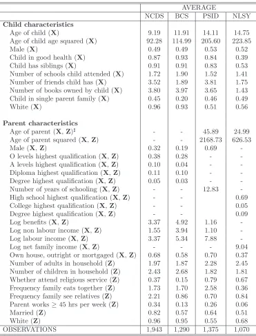
A range of additional covariates are employed where X andZ denote vectors of ex-planatory variables in the child and parent social interaction equations, respectively. In the child’s social interaction equation, variables in X consist of child covariates and parental characteristics. In particular, the child covariates are binary controls for whether the child: is male; is in good health; has any siblings; lives in a single parent family; and is white. A quadratic in the age of the child is included along with the number of schools that the child has attended, the number of friends that the child has and the number of books owned by the child. Parental controls, Z, entered into the child social interaction equation include binary indicators for whether the parent: is male; educational attainment13; and housing tenure, specifically for whether the house is owned outright or on a mortgage. We also control for household finances by includ-ing the natural logarithm of benefits, non labour income and labour income.14 Finally regional controls are also included.
For the parent’s social interaction equation, control variables inZare parent charac-teristics, some of which are also covariates in the child social interaction equation. The variables inZ consist of binary indicators for whether the parent: is white; is married; is male; highest educational attainment (as defined above); housing tenure; attends re-ligious services; and works more a 45 hour week or more. Other controls include: the number of adults in the household; the number of children in the household; controls for household finances (as defined above); the frequency that the family eats together; and the frequency that the family sees their relatives (specifically those living outside the household). In the U.S. data sets, it is possible to also include a quadratic in the age of the parent since the data is not cohort specific. Finally, we include a set of regional controls. Summary statistics for both sets of covariates,XandZ, are provided in Table 1C and full definitions are given in Table A1.
12
Ideally, individuals and their offspring would be tracked over time in each data set which would then enable the use of a panel data modelling approach in order to control for time invariant unobserved fixed effects. Limited data availability unfortunately precludes this approach.
13
In theNCDSandBCS, educational attainment is defined as highest level of educational attainment: degree (undergraduate or postgraduate); diploma level, nursing or teaching qualification; Advanced (A) level and Ordinary (O) level. O’ level qualifications are taken after eleven years of formal compulsory schooling and approximate to the U.S. honours high school curriculum. The A’ level qualification is a public examination taken by 18 year olds over a two year period studying between one to four subjects and is the main determinant of eligibility for entry to higher education in the UK. No education is the reference category. In the U.S., for theNLSY, three binary indicators are used to measure the highest level of education attained, specifically completed high school; completed some college; and attained a degree (undergraduate or postgraduate). Less than high school completion is the reference category. In thePSID, educational attainment is measured as a continuous variable by years of completed schooling.
14
4
Results
As discussed in the introduction, the majority of the economics literature in this area has focused upon the concepts of social capital and trust rather than specifically on so-cial interaction. Furthermore, the empirical evidence has concentrated on the influence of parental social capital upon the social capital of their offspring, e.g. Okumura and Usui (2010). The only exception which we are aware of is Duncan et al. (2005) who analyse mother-daughter correlations between participation in school clubs, across gen-erations using the U.S.NLSY. However, they do not investigate bi-directional influences in social interaction between parents and their offspring. Analysing correlations is the starting point for our empirical analysis whereby we estimate Eq. (31) based upon the BritishNCDS exploring the influence of parental social interaction upon the probability that their child is a member of a club. This is estimated as a univariate probit model with the results shown in Table 2 Panel A. Older children clearly have a higher proba-bility of being a member of a club in 1991, whilst there are no gender or ethnicity effects.
However, the number of close friends that the child has and the number of books owned by the child both have positive and significant impacts upon the probability of child club membership, where the latter is a potential proxy for home resources. Parental influences are dominated by the effect of the highest educational qualification obtained by 1991, where a child whose parent has a degree as their highest academic qualification (relative to no education) has a 17 percentage point higher probability of being a club member. Income effects are small and stem from household labour income. The number of clubs that the parent is a member of is as equally important as parental education in terms of magnitude, whereby a child whose parent is a member of four or more clubs (relative to no clubs) has a 22 percentage point higher probability of club membership. A possible concern with the analysis thus far is reverse causality and ideally we would either instrument parental social interaction or measure itex ante, so that the primary explanatory variable of interest predates the outcome variable.15 The latter is possible in theNCDS and, hence, in Table 2 Panel B, we measure parental club membership in 1981 and child club membership in 1991, i.e. in terms of Eq. (33a)T1> T2. The results are consistent with those in Panel A, where the membership of clubs across generations is measured concurrently, with a monotonic relationship being evident, i.e. the extent of the social interaction of the parent matters.
We now depart from the approach adopted in the existing empirical literature and explore the prediction from the theoretical framework presented in Section 2 that the social interaction of the child may also influence that of their parents. This might occur through spillover effects by reducing search costs whereby parents become involved in social events, i.e. investment in hc provides information about parental opportunities forhn (see Section 2.2). In what follows, the empirical analysis allows the causality to operate in both directions. Specifically, the social interaction of the child and that of the parent are modelled simultaneously, see Eqs. (33a) and (33b). Table 2 Panel D reports the results of modelling the probability that the child is a member of a club conditional upon the same covariates as in Panel A and binary controls for the number of clubs that the parent is a member of in 1981 (i.e. T1 > T2). The results are in line with those reported in Panels A and B indicating that parental social interaction has a statistically
15
significant impact on their offspring’s social interaction.
We now focus on the effect of the children’s social interaction on their parent’s so-cial interaction, which has largely been neglected in the literature. The corresponding parental outcome, jointly estimated with their child’s social interaction (see Table 2 Panel C), is shown in the first column of Table 3. Clearly, the value of the correlation coefficient,ρ, is statistically significant endorsing the joint modelling approach. Initially, the number of clubs that the parent is a member of is measured in 1991, i.e. at the same time as that of the child’s club membership (T3 =T4 in Eq. (33b)). We show outcomes for the probability that the parent is a member of no clubs and for the probability that the parent is a member of four or more clubs in 1991. The number of adults in the household serves to lower the probability of the parent being a member of no clubs and may proxy household resources to care for children when the parent is socialising. In terms of our theoretical model, this stems from reducing the costs associated with parental social interaction, hn, by reducing child care costs, i.e. through a reduction in pn, see Section 2. The influence of education is apparent and, where statistically significant, is monotonically associated with a lower probability of not being a member of any clubs culminating in around 21 percentage points for those parents with a degree as their highest qualification (relative to those with no education). The significant pos-itive correlation between social interaction and education is consistent with the existing empirical evidence to date, e.g. Glaeser et al. (2002). The influence of income is rela-tively small and only labour income influences the probability of the parent attending no clubs (four or more clubs) by around -2 (0.6) percentage points. As found with the social interaction of the child, there are no gender or ethnicity effects.
Controlling for the social network of the family by including the frequency that the family (i.e. household members) eat together and see relatives (i.e. outside of the household) has no influence upon the parents’ club membership. The extent to which the parent may be able to become involved in social interaction outside of the family environment may be hindered by the amount of time that they have available for so-cial activities outside work. However, including a binary control for whether the parent works a 45 hour week or more has no influence on the probability of not being a member of a club and only around a 2.7 percentage point association with decreasing the prob-ability of being a member of four or more clubs. Focusing upon the primary covariate of interest, whether the respondent’s child is a member of a club in 1991 reduces the probability that the parent is a member of no clubs by around 42 percentage points and increases the probability of being a member of four or more clubs by 8.4 percentage points. This is an effect over and above social interaction within the family and social interaction related to attendance at religious services.16
The NCDS allows us to reduce the potential for reverse causality in the parent so-cial interaction equation by measuring the child’s soso-cial interactionex ante, specifically by focusing upon the same definition of parental club membership but in 2000, i.e. in
16
terms of Eq. (33b),T3> T4. The results relating to the determinants of the probability that the child is a member of a club, shown in Table 2 Panel D, are largely unaltered. Focusing upon the corresponding parental social interaction results, in the second col-umn of Table 3, where social interaction is now measured in 2000, there are a couple of notable differences. Firstly, there is a significant gender differential in that males are approximately 5.8 percentage points less likely than females not to be a member of any clubs. Secondly, the frequency that the family visits relatives has a statistically signifi-cant positive impact upon the likelihood of not being a member of any clubs, potentially implying that social interaction inside the family might be a substitute for social inter-action outside of the family environment. The amount of leisure time available to the parent now has a relatively large effect on the probability of not being a member of any clubs, where those who work long hours are more likely not to attend clubs. However, the primary result that the social interaction of the child is positively associated with the extent of the social interaction of the parent remains robust.
The results based upon the British NCDS are arguably cohort specific since the empirical analysis focused on the social interaction of the parent when aged either 33 or 42. To investigate this further, we make use of the more recent BCS cohort data. Furthermore, the measurement of the child’s club membership in 2004 in the BCSis more detailed than that of the NCDS, as detailed in Section 3 above. The results of estimating a bivariate ordered probit as in Eqs. (33a) and (33b) are shown in Table 4, for the child’s social interaction, and Table 5, for the parent’s social interaction.17 Focusing upon the child outcome in 2004, parental social interaction is measured in 2000 soT1> T2. As compared to the results from theNCDS, the gender and ethnicity of the child are now statistically significant, although the summary statistics in Table 1C reveal similar mean characteristics. Whether the child is in good health reduces (increases) the probability of not being a member of a club (being a member of three or more clubs) by about 4.7 (4.2) percentage points. As found in theNCDS, the number of friends and the number of books that the child has are both positively associated with the extent of their club membership. The influence of parental characteristics is less evident in that there are no effects from the gender of the parent or income. If the parent belongs to two or more clubs in 2000 (relative to being a member of no clubs) then the probability that their child is a member of three or more clubs increases by 10 percentage points. Hence, the underlying results related to the child’s social interaction do not appear to be cohort specific.
Turning to the social interaction of the parent in Table 5, it is not possible to model the parental outcome at a different time to the measurement of their offspring’s social interaction due to data restrictions, hence T3 = T4. There are some differences in comparison to the results based on theNCDS in that ethnicity is clearly important, as are the number of children in the household rather than the number of adults in the household, and social interaction within the household (as proxied by the frequency the family eats together) all serve to increase the probability that the parent is a member of four or more clubs. However, the underlying result that there is a positive relationship between the social interaction of the child and that of the parent is also apparent in the BCS, where the extent of the child’s club membership does not seem to be important. Specifically, whether the child is a member of one, two or three or more clubs in 2004
17
(relative to no clubs) is associated with around a 10 percentage point increase in the probability that the parent is a member of four or more clubs. As found with theNCDS, the joint modelling approach of social interaction across generations yields an efficiency gain and suggests interdependence between the social interaction of parents and their offspring.
So far our empirical analysis supports the existence of bi-directional social interac-tion effects across generainterac-tions, which is consistent with our theoretical priors discussed in Section 2. We now further explore the robustness of these findings by investigating two U.S. datasets. Whilst, in both the PSID and NLSY, the social interaction of the child is measured in a similar fashion to that in theNCDS and theBCS, namely by the number of clubs and the probability of being a member of a club, the measurement of parental social interaction is arguably more comprehensive in the U.S. data sets. This is because, as well as being able to measure the number of clubs that a parent is a member of, information is also available upon the number of hours spent in a particular social activity. In addition, in what follows for both thePSIDandNLSY, we take advantage of timing differences in the measurement of social interaction, so as to reduce the potential for reverse causality in estimating Eqs. (33a) and (33b), i.e. T1> T2 and T3> T4.
Focusing upon thePSID, the social interaction of the child is proxied by the number of clubs they were a member of in 2002 and this is modelled with the same covariates X and Z as employed in the British data sets. Following the analysis of the British data sets, the initial measure of parental social interaction consists of binary controls for whether the parent was a member of one, two/three clubs, or four or more clubs in 1997. The results relating to the child outcome are shown in Table 6 Panel A. There are some interesting differences in comparison to the British data sets. For example, older children are more likely to attend more clubs, whereas the opposite was found when considering the BCS.18 This might be because, on average, children are slightly older in the U.S. data sets, see Table 1C. Another difference is that the gender of the child is important: males are approximately 4 (5.5) percentage points less (more) likely not to attend (attend four or more) clubs. In contrast to the British evidence, the social network of the child, as indicated by the number of friends they have, has no influ-ence upon the likelihood of club membership. There are no effects from the education of the parent and income effects, where statistically significant, are small in terms of magnitude. However, as in theBCS, whether the parent owns their home is positively associated with the probability of the child being a club member, where housing tenure may provide a proxy for the stock of wealth. As found with the British data sets, and consistent with our theoretical framework presented in Section 2, the extent of the social interaction of the parent has a positive influence upon their offspring’s social interaction. Specifically, whether the parent is a member of four or more clubs in 1997 increases the probability that their child is a member of four or more clubs in 2002 by approximately 10 percentage points.
The corresponding parental outcome is shown in Table 7 Panel A, where the proba-bility that the parent volunteers for unpaid work in 2005 is modelled conditional upon the social interaction of the child in 2002, i.e. T3> T4. The results are similar to those found using the British data sets in that there is an effect of the child’s social
interac-18
It should be noted that the types of clubs that the child is a member of differ across the BCS and
tion over and above the inclusion of controls for intra household social interaction and religious activities. The extent of the club membership of the child has a monotonic association with parental social interaction, where for a parent whose child is a mem-ber of four or more clubs, this culminates in an 8 percentage point higher probability of volunteering daily. The correlation in the error terms is statistically insignificant in the PSID and, hence, in what follows, each equation of the model (33a) and (33b) is estimated via a univariate framework.19
As mentioned above, one advantage of the PSID is that it is possible to examine the extent of the parents’ club involvement. Focusing initially on the children’s social interaction as the outcome variable, the probability of being a member of four or more clubs is increasing in the number of hours that the parent spends in clubs during 1991, see Table 6 Panel B. Given that the average number of hours that the parent volunteered in 1997 is three hours, based on this mean, this effect increases the probability that the child is a member of four or more clubs in 2002 by over 3 percentage points. In terms of the parental outcome, we consider the number of hours volunteered in 2004, (Table 7 Panel B), and the number of times the parent volunteered in 2004, (Table 7 Panel C), conditional upon the child’s social interaction in 2002 (i.e. T3 > T4). The results reveal a positive association between the extent of the child’s club membership and the time that the parent spends in unpaid voluntary work during 2004. In particular, if the child is a member of four or more clubs in 2002 then the parent volunteers an ad-ditional hour of their time (see Panel B) or volunteered an adad-ditional time (see Panel C).
In the final dataset, the NLSY, in contrast to the other three data sets, the sample of parents are all mothers. The child’s social interaction is modelled as the probability of being a member of a club in 2002. Clearly, as in the results for the other three data sets, the age of the child matters in that the likelihood of club membership is increas-ing in age, albeit at a decreasincreas-ing rate. Whilst there is no influence from the number of friends that the child has, the number of books owned is positively associated with the probability of club membership. Whether the child lives in a single parent family reduces the probability of club membership by 4 percentage points, which is an effect over and above family income. Whether the parent was a member of a club during their high school years, henceT1> T2, has a monotonic influence on the child’s probability of club attendance. In particular, if the mother attended four or more clubs during high school then the child is around 6.5 percentage points more likely to be a club member in 2002. Turning to the parent’s social interaction, we focus on the number of weeks that the parent undertook unpaid voluntary work in 2005. Mothers whose highest level of educational attainment was a degree (relative to not completing high school) are more likely to undertake voluntary work as are older individuals. Clearly, the mother’s social interaction within the family and social interaction with relatives outside of the house-hold are both important in terms of magnitude and statistical significance. Whether the mother’s child was a member of a club in 2002 has a similar influence in terms of magnitude as attending religious services, increasing the number of weeks that the parent undertook voluntary work by around a half, i.e. 3.5 days. To summarise, across the four data sets, we find convincing empirical evidence supporting a bi-directional relationship between the social interaction of parents and their offspring. Furthermore, this relationship exists in the U.S. and Great Britain and is robust across a range of
19
measures of social interaction.
5
Conclusions
In this paper, we have explored the relationship between the social interaction of parents and their offspring from both a theoretical and an empirical perspective. Our theoretical framework established possible explanations for the intergenerational transfer of social interaction whereby the social interaction of the parent may influence that of their off-spring and vice versa. The empirical evidence, based on four data sets covering both Britain and the U.S., is supportive of our theoretical priors. We find robust evidence of intergenerational links between the social interaction of parents and their offspring, which is consistent with the findings of Duncan et al. (2005) and Okumura and Usui (2010). Moreover, these links exist over and above an extensive set of controls cover-ing family background such as income and wealth, intra family social interaction and attendance at religious services. Our empirical evidence indicates that higher levels of social interaction of the parent (child) results in higher levels of social interaction of the child (parent). Hence, it would appear that positive bi-directional intergenerational effects exist in social interaction. Our findings contribute more generally to the existing literature on intergenerational economic outcomes, such as earnings (e.g Solon, 1999), formal educational outcomes (e.g. Blandenet al., 2007) and test scores (e.g. Brownet al., 2011).
References
Angrist, J. and Pischke, J.-S. (2009). Mostly Harmless Econometrics: An Empiri-cists Companion. Princeton: Princeton University Press.
Beck, P. and Jennings, M. (1982). Pathways to participation. American Political Science Review,76, 94–108.
Becker, G. S.(1965). A theory of the allocation of time.Economic Journal,75, 493– 517.
—(1974). A theory of social interactions.Journal of Political Economy,82, 1063–1093.
Bentham, J.(1789).Principles of Morals and Legislation. Oxford: Clarendon.
Blanden, J.,Gregg, P.andMacmillan, L.(2007). Accounting for intergenerational income persistence: noncognitive skills, ability and education.Economic Journal,117, C43–C60.
Bowles, S., Gintis, H. and Osborne, M. (2001). The determinants of earnings: A behavioral approach. Journal of Economic Literature,39, 1137–1176.
Brown, S., McIntosh, S. and Taylor, K.(2011). Following in your parents’ foot-steps? Empirical analysis of matched parent-offspring test scores.Oxford Bulletin of Economics and Statistics,73(1), 40–58.
—and—(2009). Social interaction and children’s academic test scores: Evidence from the national child development study.Journal of Economic Behavior & Organization, 71(2), 563–574.
Cunha, F. and Heckman, J. (2007). The technology of skill formation. American Economic Review,97, 31–47.
Dohmen, T. J.,Falk, A.,Huffman, D.andSunde, U.(2007).The Intergenerational Transmission of Risk and Trust Attitudes. IZA Discussion Papers 2380, Institute for the Study of Labor (IZA). Forthcoming in the Review of Economic Studies.
Duncan, G.,Kalil, A.,Mayer, S.,Tepper, R. and Payne, M.(2005). The apple does not fall far from the tree. In M. Osborne, S. Bowles and H. Gintis (eds.),Unequal chances: Family background and economic success, New York: Russell Sage.
Glaeser, E. L.,Laibson, D. and Sacerdote, B. (2002). An economic approach to social capital.Economic Journal,112 (483), 437–458.
Guiso, L., Sapienza, P. and Zingales, L. (2008). Social capital as good culture. Journal of the European Economic Association,6, 295–320.
Iannaccone, L. R.(1998). Introduction to the economics of religion. Journal of Eco-nomic Literature,36(3), 1465–1495.
Jennings, M.and Stoker, L. (2004). Social trust and civic engagement across time and generations. Acta Politica,39, 342–379.
Marshall, A.(1962). Principles of Economics. London: Macmillan, 8th edn.
Michael, R. T.andBecker, G. S.(1973). On the new theory of consumer behavior. Swedish Journal of Economics,75, 378–396.
Okumura, T.andUsui, E.(2010).Do Parents’ Social Skills Influence Their Children’s Sociability? IZA Discussion Papers 5324, Institute for the Study of Labor (IZA).
Putnam, R.(2000). Bowling Alone: The Collapse and Revival of American Commu-nity. New York: Simon and Schuster.
Sacerdote, B.and Glaeser, E. L.(2001).Education and Religion. NBER Working Papers 8080, National Bureau of Economic Research, Inc.
Sajaia, Z. (2008). BIOPROBIT: Stata module for bivariate ordered probit regression. Statistical Software Components S456920, Boston College Department of Economics.
Solon, G.(1999). Intergenerational mobility in the labour market. In O. Ashenfelter and D. Card (eds.),Handbook of Labor Economics, vol. 3, Amsterdam: North-Holland.
Table 1A: Summary Statistics - Dependent Variables
AVERAGE
NCDS BCS PSID NLSY
Child outcomeSOCchild i,T1
Member of a club in 1991{0,1} (T1=1991) 0.63 - - -Number of clubs a member of in 2004{0,≥3} (T1=2004) - 1.46 - -Number of clubs a member of in 2002{0,≥4} (T1=2002) - - 2.09 -Member of a club in 2002{0,1} (T1=2002) - - - 0.25
Parent outcomeSOCj,Tparent3
Number of clubs a member of in 1991{0,≥3} (T3=1991) 1.01 - - -Number of clubs a member of in 2000{0,≥3} (T3=2000) 0.77 - - -Number of clubs a member of in 2004{0,≥4} (T3=2004) - 1.40 - -Voluntary work in 2005{0 =never,3 =daily}(T3=2004) - - 0.66 -Number of times volunteered in 2005{0,100}(T3=2004) - - 2.25 -Number of hours volunteered in 2005{0,2920}(T3=2004) - - 69.34 -Number of weeks volunteered in 2006{0,52}(T3=2005) - - - 6.05
OBSERVATIONS 1,943 1,290 1,375 1,070
Table 1B: Summary Statistics - Social Interaction Independent Variables
AVERAGE
NCDS BCS PSID NLSY
Child outcome, parental social interactionSOCj,Tparent2
Member of 1 club in 1991{0,1} (T2=1991) 0.36 - - -Member of 2-3 clubs in 1991{0,1}(T2=1991) 0.23 - - -Member of 4 or more clubs in 1991{0,1}(T2=1991) 0.03 - - -Member of 1 club in 1981{0,1} (T2=1981) 0.31 - - -Member of 2-3 clubs in 1981{0,1}(T2=1981) 0.23 - - -Member of 4 or more clubs in 1981{0,1}(T2=1981) 0.03 - - -Member of 1 club in 2000{0,1} (T2=2000) - 0.23 - -Member of 2 or more clubs in 2000{0,1}(T2=2000) - 0.05 - -Member of 1 club in 1997{0,1} (T2=1997) - - 0.26 -Member of 2-3 clubs in 1997{0,1}(T2=1997) - - 0.23 -Member of 4 or more clubs in 1997{0,1}(T2=1997) - - 0.07 -Member of 1 club in high school{0,1} - - - 0.25 Member of 2-3 clubs in high school{0,1} - - - 0.28 Member of 4 or more clubs in high school{0,1} - - - 0.05
Parent outcome, child social interactionSOCchild j,T4
Member of a club in 1991{0,1} (T4=1991) 0.63 - - -Member of 1 club in 2004{0,1} (T4=2004) - 0.39 - -Member of 2 clubs in 2004{0,1} (T4=2004) - 0.27 - -Member of 3 or more clubs in 2004{0,1}(T4=2004) - 0.18 - -Member of 1 club in 2002{0,1} (T4=2002) - - 0.21 -Member of 2-3 clubs in 2002{0,1}(T4=2002) - - 0.44 -Member of 4 or more clubs in 2002{0,1}(T4=2002) - - 0.20 -Member of a club in 2002{0,1} (T4=2002) - - - 0.25
[image:25.595.94.517.423.772.2]Table 1C: Summary Statistics - Independent Variables
AVERAGE
NCDS BCS PSID NLSY
Child characteristics
Age of child (X) 9.19 11.91 14.11 14.75
Age of child age squared (X) 92.28 114.99 205.60 223.85
Male (X) 0.49 0.49 0.53 0.52
Child in good health (X) 0.87 0.93 0.84 0.39
Child has siblings (X) 0.91 0.91 0.83 0.53
Number of schools child attended (X) 1.72 1.90 1.52 1.41 Number of friends child has (X) 3.52 1.89 3.81 1.75 Number of books owned by child (X) 3.80 3.97 3.65 1.43 Child in single parent family (X) 0.45 0.20 0.46 0.49
White (X) 0.96 0.93 0.51 0.56
Parent characteristics
Age of parent (X,Z)♯ - - 45.89 24.99
Age of parent squared (X,Z) - - 2168.73 626.53
Male (X,Z) 0.32 0.19 0.69
-O levels highest qualification (X, Z) 0.38 0.28 - -A levels highest qualification (X,Z) 0.10 0.04 - -Diploma highest qualification (X,Z) 0.11 0.10 - -Degree highest qualification (X,Z) 0.05 0.03 - -Number of years of schooling (X,Z) - - 12.83 -High school highest qualification (X,Z) - - 0.69 College highest qualification (X,Z) - - 0.05 Degree highest qualification (X,Z) - - 0.09
Log benefits (X,Z) 3.37 4.92 1.16
-Log non labour income (X,Z) 1.55 3.94 1.10 -Log labour income (X,Z) 3.37 5.34 7.88
-Log net family income (X,Z) - - - 9.04
Own house, outright or mortgaged (X,Z) 0.68 0.58 0.70 0.37 Number of adults in household (Z) 1.97 1.87 2.28 2.45 Number of children in household (Z) 2.43 2.68 1.82 1.81 Whether attend religious service (Z) 0.37 0.15 0.79 0.67 Frequency family eats together (Z) 1.73 1.70 2.58 0.36 Frequency family see relatives (Z) 2.21 0.86 0.70 0.84 Parent works≥45 hrs per week (Z) 0.34 0.13 0.26 0.06
Married (Z) 0.82 0.57 0.64 0.51
White (Z) 0.96 0.95 0.55 0.68
OBSERVATIONS 1,943 1,290 1,375 1,070
♯All parents in theNCDS (BCS) are 33 in 1991 (34 in 2004), there is no variation