This is a repository copy of Stability of synchronized motions of inverter-based microgrids
under droop control.
White Rose Research Online URL for this paper:
http://eprints.whiterose.ac.uk/92372/
Version: Accepted Version
Proceedings Paper:
Schiffer, J, Ortega, R, Astolfi, A et al. (2 more authors) (2014) Stability of synchronized
motions of inverter-based microgrids under droop control. In: IFAC Proceedings Volumes.
19th IFAC World Congress, 24-29 Aug 2014, Cape Town, South Africa. Elsevier , pp.
6361-6367. ISBN 978-3-902823-62-5
https://doi.org/10.3182/20140824-6-ZA-1003.00863
© 2014 IFAC. Published by Elsevier Ltd. Licensed under the Creative Commons
Attribution-NonCommercial-NoDerivatives 4.0 International
http://creativecommons.org/licenses/by-nc-nd/4.0/
[email protected] https://eprints.whiterose.ac.uk/
Reuse
Unless indicated otherwise, fulltext items are protected by copyright with all rights reserved. The copyright exception in section 29 of the Copyright, Designs and Patents Act 1988 allows the making of a single copy solely for the purpose of non-commercial research or private study within the limits of fair dealing. The publisher or other rights-holder may allow further reproduction and re-use of this version - refer to the White Rose Research Online record for this item. Where records identify the publisher as the copyright holder, users can verify any specific terms of use on the publisher’s website.
Takedown
If you consider content in White Rose Research Online to be in breach of UK law, please notify us by
Stability of Synchronized Motions of
Inverter–Based Microgrids Under Droop
Control
Johannes Schiffer∗ Romeo Ortega∗∗ Alessandro Astolfi∗∗∗ J¨org Raisch∗,∗∗∗∗ Tevfik Sezi3
∗Technische Universit¨at Berlin, Germany
(e-mail: [email protected])
∗∗Laboratoire des Signaux et Syst´emes, SUPELEC, France
(e-mail: [email protected])
∗∗∗Department of Electrical and Electronic Engineering, Imperial
College London, London SW7 2AZ, U.K. & Dipartimento di Ing. Civile e Ing. Informatica, University of Rome, Tor Vergata, 00133
Rome, Italy (e-mail: [email protected])
∗∗∗∗Max-Planck-Institut f¨ur Dynamik komplexer technischer Systeme,
Germany (e-mail: [email protected])
3Siemens AG, Germany (e-mail: [email protected])
Abstract:We consider the problems of frequency stability, voltage stability and power sharing in droop–controlled inverter–based microgrids with meshed topologies and dominantly inductive power lines. Assuming that the conductances in the microgrid can be neglected, a port– Hamiltonian description of a droop–controlled microgrid is derived. The model is used to establish sufficient conditions for local stability. Furthermore, we propose a condition for the controller parameters such that a desired steady–state active power distribution is achieved. The robustness of the stability condition with respect to the presence of conductances is analyzed via a simulation example based on the CIGRE benchmark medium voltage distribution network.
Keywords:microgrid stability, inverters, droop control, port–Hamiltonian systems
1. INTRODUCTION
The increasing amount of renewable energy sources present in the electrical grid requires new technical concepts to ensure a safe and reliable operation. Two main reasons for this are: (i) most renewable generation sources are small–scale distributed generation (DG) units connected at the low (LV) and medium voltage (MV) levels; (ii) a large portion of these DG units are interfaced with the network via AC inverters, the physical characteristics of which largely differ from the characteristics of conventional synchronous generators (SGs).
In that regard, microgrids represent a promising near– time concept to facilitate the integration of renewable DG sources, see Lasseter (2002). A microgrid gathers a combination of generation units, loads and energy storage elements at distribution level into a locally controllable system, which can be operated in isolation from the main transmission system. A microgrid in the latter operation mode is called an autonomous or islanded microgrid. This paper addresses three important performance criteria in such networks: frequency stability, voltage stability and power sharing. Here, power sharing is understood as the ability of the local controls of the individual generation sources to achieve a desired steady–state distribution of their power outputsrelativeto each other, while satisfying the load demand in the network. The relevance of this control objective lies within the fact that it allows to pre-specify the utilization of the generation units in operation.
⋆ Partial support from the HYCON2 Network of excellence (FP7
ICT 257462) is acknowledged.
A widely used, though heuristic, solution for the problem of active power sharing in conventional power systems is droop control, see Kundur (1994). In the case of an SG, droop control is a decentralized proportional control, which sets the mechanical output power in dependency of the relative deviations of the rotational speed of the SG. Given its successful application in such systems, this technique has been adapted to inverter–based networks in Chandorkar et al. (1993); Coelho et al. (2002).
Under the assumption of constant voltage amplitudes, conditions for frequency stability and power sharing for radial microgrids with first–order inverter models and purely inductive power lines have recently been presented in Simpson-Porco et al. (2013a). Conditions for voltage stability for a parallel microgrid with inductive power lines have been derived in Simpson-Porco et al. (2013b) under the assumption of small or constant angle differences. However, and as pointed out in Guerrero et al. (2013), most work on microgrid stability has so far focussed on radial microgrids, while stability of microgrids with meshed topologies and decentralized controlled units is still an open research area. In that regard, and under the assumption of constant voltage amplitudes, analytic synchronization conditions for a lossy meshed microgrid with distributed rotational and electronic generation are derived in Schiffer et al. (2013) using ideas from second or-der consensus algorithms. A decentralized LMI–based con-trol design for lossy meshed inverter–based networks guar-anteeing overall network stability for a nonlinear model considering variable voltage amplitudes and phase angles is provided in Schiffer et al. (2012).
The main contribution of this paper is to give sufficient conditions on the control parameters to ensure local stabil-ity of droop–controlled inverter–based microgrids operated with the control laws given in Chandorkar et al. (1993). We hereby consider networks with general meshed topol-ogy and inverter models with variable frequencies as well as variable voltage amplitudes. Since the synchronization frequency is the same for all DG units and their dynamics depend on the angle differences, it is possible to translate— via a time–dependent coordinate shift—the synchroniza-tion objective into a (standard) equilibrium stabilizasynchroniza-tion problem, which is the approach adopted here.
Specifically, we follow the interconnection and damping assignment passivity–based control approach of Ortega et al. (2002) to represent the lossless microgrid in port– Hamiltonian form, see van der Schaft (2000). This allows to easily identify the energy–Lyapunov function and give conditions for stability of the synchronization equilibrium state. In contrast to Simpson-Porco et al. (2013a,b); Schif-fer et al. (2013), no assumptions of constant voltage am-plitudes or small phase angle differences are made. The remainder of the paper is organized as follows. The network model is presented in Section 2. The inverter model and the droop control are introduced in Section 3. Sufficient conditions for local stability for lossless micro-grids are established in Section 4. In Section 5 we propose a selection of the droop gains and setpoints that ensures the DG units share (in steady–state) the active power according to a specified pattern. The robustness of our stability condition with respect to model uncertainties,e.g.
conductances, is evaluated in Section 6 with a simulation example based on the CIGRE (Conseil International des Grands R´eseaux Electriques) benchmark MV distribution network, see Rudion et al. (2006). The paper is wrapped– up with some conclusions and future work in Section 7. This paper is an abridged version of Schiffer et al. (2014), in which further results on properties of droop–controlled microgrids, also under the presence of conductances, are given. These include, among others, a proof that for all practical choices of the parameters of the droop controllers global boundedness of trajectories is ensured. In addition, based on this result, a relaxed stability condition for a specific gain selection in a lossless network is derived. Furthermore, extensive simulation studies illustrating the theoretical analysis are provided.
Notation. We define the sets R≥0:={x∈R|x≥0}, R>0:={x∈R|x >0},R<0:={x∈R|x <0},S:= [0,2π)
and ¯n:={1, . . . , n}.Given a setU :={ν1, . . . , νn},the
no-tationi∼ U denotes “for alli∈ U”. Letx:= col(xi)∈Rn
denote a vector with entries xi for i ∼ n, 0¯ n ∈ Rn
the zero vector, 1n ∈ Rn the vector with all ones and
diag(ai), i ∼ n,¯ an n×n diagonal matrix with diagonal
entriesai. Letjdenote the imaginary unit. The transpose
of the gradient of a functionf :Rn→Ris denoted by∇f.
2. NETWORK MODEL
We consider a generic meshed network model in which loads are represented by constant impedances. This leads to a set of nonlinear differential–algebraic equations. It is then possible to eliminate all algebraic equations cor-responding to loads via a process called Kron reduction, see Kundur (1994), and obtain a set of pure differential equations. We assume this process has been carried out and work with the Kron–reduced network.
In the Kron–reduced microgrid, composed ofnnodes, each node represents a DG unit interfaced via an AC inverter. We denote the set of network nodes by ¯n and associate a time–dependent phase angle δi : R≥0 → S, as well
as a time–dependent voltage amplitude Vi:R≥0→R>0
to each node i ∈ n¯ in the microgrid. We further-more assume that the power lines of the microgrid are dominantly inductive. Then, two nodes i and k of the microgrid are connected via a complex nonzero admit-tanceYik:=Gik+jBik∈Cwith conductanceGik∈R>0
and susceptance Bik∈R<0. For convenience, we define
Yik:= 0 wheneveriandkare not directly connected via an
admittance. The set of neighbors of a nodei∈n¯is given by Ni:={k
k∈¯n, k6=i , Yik6= 0}.For ease of notation, we
write angle differences asδik(t) :=δi(t)−δk(t) and define
the vectorsδ(t) := col(δi(t))∈Sn, ω(t) := col(ωi(t))∈Rn
andV(t) := col(Vi(t))∈Rn,where ˙δ(t) =ω(t).
Following Kundur (1994), the overall active and reactive power flowsPi:Sn×Rn>0→RandQi:Sn×Rn>0→Rat
a nodei∈n¯ are given by1 Pi=GiiVi2−
X
k∼Ni
ViVk(Gikcos(δik) +Biksin(δik)),
Qi=−BiiVi2− X
k∼Ni
ViVk(Giksin(δik)−Bikcos(δik)),
(1)
with
Gii := ˆGii+ X
k∼Ni
Gik, Bii := ˆBii+ X
k∼Ni
Bik, (2)
where ˆGii ∈ R>0 and ˆBii ∈ R<0 denote the shunt
con-ductance, respectively shunt susceptance, at node i. The apparent power flow is given bySi=Pi+jQi.We associate
to each inverter its power ratingSN
i ∈R>0, i∼n.¯
We assume that the microgrid is connected,i.e.that for all pairs{i, k} ∈¯n×n, i¯ 6=k,there exists an ordered sequence of nodes fromitoksuch that any pair of consecutive nodes in the sequence are connected by a power line represented by an admittance. This assumption is reasonable for a microgrid, unless severe line outages separating the system into several disconnected parts occur. Since we are mainly concerned with dynamics of generation units, we express all power flows in ”Generator Reference Arrow System”.
1
3. INVERTER MODEL AND DROOP CONTROL
The inverters are modeled as AC voltage sources with controllable amplitude and frequency, see Lopes et al. (2006)2. The frequency regulation is assumed
instanta-neous, but the voltage control is assumed to happen with a delay represented by a first order filter with time constant τVi ∈ R>0. Then, the dynamics of the inverter at node
i∈¯ncan be modeled as ˙ δi=uδi,
τViV˙i=−Vi+u
V
i,
(3)
where uδ
i :R≥0→R anduVi :R≥0→Rare controls. The
active and reactive power outputs are assumed to be measured and passed through filters with time constant τPi ∈ R>0 and Pi and Qi given in (1), see Coelho et al.
(2002); Pogaku et al. (2007),i.e.
τPiP˙
m i =−P
m i +Pi,
τPiQ˙
m
i =−Qmi +Qi.
(4)
Differently from SGs, inverters do not have an inherent physical relation between frequency and generated active power. Droop control attempts at artificially establishing such relation, since it is desired in many applications, see Engler (2005). The typical (heuristic) argument for the derivation of the droop control laws for inverter–based systems with dominantly inductive power lines is as fol-lows, see Chandorkar et al. (1993); Engler (2005). Assume dominantly inductive power lines, i.e.Gik≈0,and small
phase angle differencesδik. Then, it follows from the power
flow equations (1) that the active power flowPi is mainly
affected by the phase angle differences, while the reac-tive power flow Qi is mostly influenced by differences in
voltage amplitudes. This motivates proportional feedback laws coupling the frequency with the active power and the voltage with the reactive power, namely
uδ
i =ωd−kPi(P
m i −Pid),
uV i =V
d
i −kQi(Q
m i −Q
d i),
(5)
where ωd ∈R
>0 is the desired (nominal) frequency,Vid ∈
R>0 the desired (nominal) voltage amplitude,kPi ∈ R>0
andkQi ∈R>0are the frequency and voltage droop gains,
Pm
i :R≥0→Rand Qmi : R≥0 →Rthe measured powers
andPd
i ∈RandQdi ∈Rtheir desired setpoints. Inserting
(5) in (3) together with (4) yields the closed–loop system
˙
δi=ωd−kPi(P
m i −Pid),
τPiP˙
m i =−P
m i +Pi,
τViV˙i=−Vi+V
d
i −kQi(Q
m i −Q
d i),
τPiQ˙
m
i =−Qmi +Qi.
(6)
Since, in general, τVi ≪ τPi, we assume τVi = 0 in the
sequel. In addition, we rewrite the system (6) following Schiffer et al. (2013) and obtain
˙ δi=ωi,
τPiω˙i=−ωi+ω
d−k
Pi(Pi−P
d i),
τPiV˙i=−Vi+V
d
i −kQi(Qi−Q
d i),
(7)
2
An underlying assumption to this model is that whenever the inverter connects an intermittent renewable generation source,e.g.,a
photovoltaic plant or a wind plant, to the network, it is equipped with some sort of storage (e.g., flywheel, battery). Thus, it can increase
and decrease its power output in a certain range.
whereωi denotes the inverter frequency. Defining
Pd:=col(Pid)∈R n
, P := col(Pi)∈Rn,
Qd:=col(Qd
i)∈Rn, Q:= col(Qi)∈Rn,
Vd:=col(Vd i )∈R
n, T := diag(τ Pi)∈R
n×n,
KP :=diag(kPi)∈R
n×n, K
Q := diag(kQi)∈R
n×n,
(8)
we can write the system (7) compactly as ˙
δ=ω,
Tω˙ =−ω+1nωd−KP(P−Pd),
TV˙ =−V +Vd−K
Q(Q−Qd),
(9)
with power flowsP andQgiven in (1).
Remark 3.1. Note that Pd
i can also take negative values
whenever an inverter connects a storage device to the network. Then, the storage device functions as a frequency and voltage dependent load, which is charged in depen-dency of the excess power available in the network. We refer to such operation mode as charging mode.
Remark 3.2. There are several other alternative droop
control schemes proposed in the literature, e.g., Zhong (2013); Guerrero et al. (2013). The one given in (5) is the most common one for dominantly inductive networks. We therefore restrict our analysis to these control laws, commonly referred to as “conventional droop control”.
4. STABILITY FOR LOSSLESS MICROGRIDS
In this section conditions for stability for lossless
micro-grids, i.e.Gik = 0 for all i ∈ ¯n, k ∈ n,¯ are derived. We
therefore make the following assumption on the network admittances.
Assumption 4.1. Gik= 0 and Bik≤0, i∼n, k¯ ∼n.¯
This assumption can be justified for certain microgrids, especially on the MV level, as follows: while the line admit-tance in MV and LV networks has usually a non–negligible resistive part, typically the inverter output impedance is inductive (due to the inductance of the output filter and/or the presence of an output transformer). Then, the inductive parts dominate the resistive parts.
We only consider such microgrids and absorb the inverter output admittance (together with the possible transformer admittance), ˜Yik, into the line admittances, Yik, while
neglecting all resistive effects. In the present case this assumption is further justified, since the droop control laws introduced in (5) are mostly used in networks with domi-nantly inductive admittances, see Guerrero et al. (2013).
Under Assumption 4.1, the power flows (1) reduce to
Pi= X
k∼Ni
|Bik|ViVksin(δik),
Qi=|Bii|Vi2− X
k∼Ni
|Bik|ViVkcos(δik).
Remark 4.2. The need to introduce the, sometimes
instead of constant impedances in the so–called structure preserving power system models. However, in the presence of variable voltages the load models are usually, somehow artificially, adapted to fit the theoretical framework used for the construction of energy–Lyapunov functions, see
e.g., Davy and Hiskens (1997).
To establish our main result we need the following natural assumption on existence of a synchronized motion of system (9).
Assumption 4.3. There exist constants δs ∈ Θ, ωs ∈ R
andVs∈Rn
>0, where
Θ :=nδ∈Sn|δik|<
π
2, i∼n, k¯ ∼ Ni
o
,
such that the system (9) possesses for all t ≥ 0 a synchronized motion given by3
δ∗(t) = mod2π{δs+ 1nω
st}, ω∗(t) = 1 nω
s, V∗(t) =Vs, (10)
satisfiying
1nωs−1nωd+KP[P(δs, Vs)−Pd] = 0,
Vs−Vd+K
Q[Q(δs, Vs)−Qd] = 0.
Remark 4.4. It is well–known that in lossless power
sys-temsP i∼¯nP
s
i = 0. Hence, the synchronization frequency
can be uniquely determined by replacing the synchronized motion (10) in (7) and adding up all nodes, yielding
ωs=ωd+ P
i∼n¯P
d i P
i∼n¯k1Pi
.
It follows that, for anyi∈¯n,
ωs−ωd−k PiP
d i =
X
k∼n,k6¯ =i
kPi
kPk
ωd−ωs+k PkP
d k
. (11)
4.1 Error dynamics
To establish conditions on the setpoints and gains of the controller (5) such that the synchronized motion (10) is stable, it is convenient to introduce the error coordinates
˜
ω(t) :=ω(t)−1nωs, δ(t) :=˜ δ(0) + Z t
0
˜ ω(τ)dτ
and to study stability of the synchronized motion (10) in the coordinates col(˜δ(t),ω(t), V˜ (t))∈Rn×Rn×Rn>0.
Note that the power flowsP andQin (8) are invariant to a uniform shift of all angles. Hence,δ∗is only unique up to such a shift and convergence to the desired synchronized motion (10) (up to a uniform shift of all angles) does not depend on the value of the angles, but only on their differences. Therefore, we can arbitrarily choose one node, say the n–th node, as a reference node, express ˜δi,
i∈¯n\ {n} relative to ˜δn via the state transformation
θ:=Rδ,˜ R:= [I(n−1) −1(n−1)] (12)
and study convergence to the synchronized motion (10) in the reduced system of order 3n−1 withθ= col(θ1, . . . , θn−1)
replacing ˜δ.
To simplify notation, we define theconstant4 θ
n:= 0,the
shorthand θik :=θi−θk (which clearly verifies θik ≡δik
fork6=nandθin≡θi) and the constants
c1i:=ω
d−ωs+k PiP
d
i, c2i:=V
d
i +kQiQ
d
i, i∼¯n. (13)
3
The operator mod2π{·} : R → [0,2π), is defined as follows:
y = mod2π{x} yields y = x −k2π for some integer k with
sign(y) = sign(x) andy∈[0,2π). 4
The constantθnis not part of the state vectorθ.
In the new coordinates col(θ,ω, V˜ )∈Rn−1×Rn×Rn>0the
dynamics (9) take for thei–th node,i∈n¯\ {n},the form ˙
θi= ˜ωi−ω˜n,
τPiω˙˜i=−ω˜i−kPi
X
k∼Ni
ViVk|Bik|sin(θik) +c1i, (14)
τPiV˙i=−Vi−kQi |Bii|V
2
i − X
k∼Ni
ViVk|Bik|cos(θik)+c2i,
while the dynamics of the reference nodenare given by τPnω˙˜n=−ω˜n+kPn
X
k∼Nn
VnVk|Bnk|sin(θk) +c1n, (15)
τPnV˙n=−Vn−kQn|Bnn|V
2
n− X
k∼Nn
VnVk|Bnk|cos(θk)
+c2n.
This reduced system has an equilibrium at xs:= col(θs,0
n, V
s), (16)
the asymptotic stability of which implies asymptotic con-vergence of all trajectories of the system (9) to the syn-chronized motion (10) up to a uniform shift of all angles.
4.2 Main result
To present the main stability result it is convenient to introduce the matricesL ∈R(n−1)×(n−1),W ∈R(n−1)×n,
D ∈Rn×n andT(θs)∈Rn×n defined in Appendix A.
Lemma 4.5. Consider system (9), (1) with Assumptions 4.1
and 4.3. ThenL>0.
Proof. Consider the vector P defined in (8) under As-sumption 4.1 and let ˜Lbe given by
˜ L:= ∂P
∂δ
(δs,Vs)∈R
n×n
with entries given in Appendix A. Under the given as-sumptions, and recalling that the microgrid is connected by assumption, ˜L is a symmetric Laplacian matrix of a connected graph with the properties, see Simpson-Porco et al. (2013a); Schiffer et al. (2013)
˜
Lγ1n= 0, v⊤Lv >˜ 0, ∀v∈Rn\ {v=γ1n}, γ∈R. (17)
Recall the matrix R defined in (12), let r := h0⊤(n−1) 1
i
and note that ˜
LhRri
−1
= ˜L
I
(n−1) 1(n−1)
0⊤(n−1) 1
=
L 0 n−1
b⊤ 0
, (18)
where b= col(˜lin)∈R(n−1), i∼¯n\ {n}. It follows from
(17) and (18) that for any ˜v:= col(ϑ,0)∈Rn, ϑ∈R(n−1)
˜ v⊤L˜hRri
−1
˜
v= ˜v⊤L˜˜v=ϑ⊤Lϑ >0.
Moreover,Lis symmetric. Hence,L>0.
We are now ready to state our main result.
Proposition 4.6. Consider the system (9), (1) with
As-sumptions 4.1 and 4.3. FixτPi, kPi andP
d
i. SelectVid, kQi
andQd
i such that
D+T(θs)− W⊤L−1W>0. (19)
Then the equilibriumxs= col(θs,0
n, Vs) of system (14)–
(15) is locally asymptotically stable.
energy–Lyapunov function. Defining x:= col(θ,ω, V˜ ),the system (14)–(15) can be written as
˙
x= (J−R(x))∇H (20) with HamiltonianH :R(n−1)×Rn×Rn
>0→Rgiven by
H(x) =
n X
i=1
τPi
2kPi
˜ ω2i +
1 kQi
(Vi−c2iln(Vi)) +
1 2|Bii|V
2
i
−1 2
X
k∼Ni
ViVk|Bik|cos(θik)
−
n−1
X
i=1
c1i
kPi
θi. (21)
The interconnection and damping matrices are
J =
0
(n−1)×(n−1) J
−J⊤ 0
2n×2n
, R= diag(0(n−1), Rω, RV),
whereJ =hJK − kPn
τPn1(n−1) 0(n−1)×n
i
,
JK= diag
kPk
τPk
∈R(n−1)×(n−1), k∼n¯\ {n},
Rω= col
kPi
τ2
Pi
∈Rn, RV = col
kQiVi
τPi
∈Rn,
i∼n.¯ Notice that J =−J⊤ andR≥0 and hence
˙
H =−(∇H)⊤R∇H ≤0. (22) Consequently, xs is a stable equilibrium of system (14)–
(15) if H(x) has a strict local minimum at the equi-librium xs. The latter can be ensured by showing that
∇H(xs) = 0
(3n−1)and
∂2H(x) ∂x2
xs >0. That the first
re-quirement is satisfied follows from
∂H
∂θ
xs
⊤
= col ai−
c1i
kPi
∈R(n−1),
∂H
∂ω˜
xs
⊤
= 0n,
∂H
∂V
xs
⊤
= col
−bl+|Bll|Vls+
1 kQl
1−c2l
Vs l
∈Rn,
wherei∼¯n\ {n}, l∼n¯ and
ai:= X
k∼Ni
VisV s
k|Bik|sin(θiks), bl:= X
k∼Nl
Vks|Blk|cos(θslk).
Evaluating the Hessian ofH(x) atxs yields
∂2H(x)
∂x2
xs =
" L 0
(n−1)×n W
0n×(n−1) A 0n×n
W⊤ 0
n×n D+T(θs) #
where L, W, D and T(θs) are given in (A.1), (A.2) and
A := diag(τPi/kPi)∈ R
n×n. Since A is positive definite,
the Hessian is positive definite if and only if the submatrix
L W
W⊤ D+T(θs)
(23)
is positive definite. Now, Lemma 4.5 implies that, under the standing assumptions, L is positive definite. Hence, the matrix (23) is positive definite if and only if
D+T(θs)− W⊤L−1W>0,
which is condition (19). Note that from (2), it follows that T(θs) is positive semidefinite.
From (22) and the fact thatR(x)≥0, it follows that the equilibrium xsis asymptotically stable if
R(x(t))∇H(x(t))≡0(3n−1) ⇒t→∞lim x(t) =x
s
(24)
along the trajectories of the system (20). This implies ∂H
∂ω˜ = 0n, ∂H ∂V = 0n.
The first condition implies ˜ω = 0n and, hence, θ is
con-stant. The second condition implies V constant. Conse-quently, the invariant set where ˙H(x(t))≡ 0 is an equi-librium. To prove that this is the desired equilibrium xs
we recall thatxsis an isolated minimum ofH(x). Hence,
there is a neighborhood ofxs where no other equilibrium
exists, completing the proof.
Condition (19) has the following physical interpretation: the droop control laws (5) establish a feedback intercon-nection linking the phase anglesδ,respectivelyθ, with the active power flows P, as well as the voltages V with the reactive power flowsQ.
The matrices L and T(θs) represent then the network
coupling strengths between the phase angles and the active power flows, respectively, the voltages and the reactive power flows. In the same way, W can be interpreted as a local cross–coupling strength originating from the fact that P 6= P(δ) and Q 6= Q(V), but P = P(δ, V) and Q=Q(δ, V).
Condition (19) states that to ensure local stability of the equilibrium xs defined in (16) the couplings represented
byLandT(θs) have to dominate over the cross–couplings
of the power flows contained inW. If that is not the case the voltage variations have to be reduced by reducing the magnitudes of the gainskQi, i∈n.¯
Another possibility is to adapt Qd
i and Vid. This does,
however, not seem as appropriate in practice since these two parameters are typically setpoints provided by a supervisory control, which depend on the nominal voltage of the network and the expected loading conditions.
Remark 4.7. To see that (20) is indeed an equivalent
representation of (14)–(15), note that the part of the dynamics of ˜ωn in (15) resulting fromJ∇H is
kPn
τPn
1⊤(n−1)
∂H
∂θ
⊤
=kPn
τPn
X
k∼Nn
VnVk|Bnk|sin(θk)− n−1
X
i=1
c1i
kPi
,
sincePn−1 i=1
P
k∼Ni,k6=nViVk|Bik|sin(θik) = 0. From (11),
we moreover have that
c1n=ω
d−ωs+k PnP
d n =−
n−1
X
i=1
kPn
kPi
c1i.
The remaining term in ˜ωnis contributed by the dissipation
partR∇H.
Remark 4.8. The analysis reveals that stability properties
of the lossless microgrid (9) are independent of the fre-quency droop gainskPi,the active power setpointsP
d i and
the low pass filter time constants τPi, and only condition
(19) is imposed on Vd
i , kQi and Q
d
i. In that regard, the
result is identical to those derived for lossless first–order inverter models in Simpson-Porco et al. (2013a) and loss-less second–order inverter models in Schiffer et al. (2013), both assuming constant voltage amplitudes.
5. ACTIVE POWER SHARING
Definition 5.1. Letχi∈R>0denote weighting factors and
Ps
i the steady–state active power flow, i ∼n. Then, two¯
inverters at nodes i and k are said to share their active powers proportionally if
Ps i
χi
= P
s k
χk
. (25)
A possible power sharing performance criterion would be, for example, χi = SiN, i ∼ n,¯ where SiN ∈ R>0 is the
nominal power rating of inverteri.
Lemma 5.2. Consider the system (9), (1). Assume that
it possesses a synchronized motion with synchronization frequencyωs∈R
>0.Then all inverters, the power outputs
of which satisfy sign(Ps
i) = sign(Pks),achieve proportional
active power sharing if the gainskPiandkPkand the active
power setpointsPd
i andPkd are chosen such that
kPiχi=kPkχk andkPiP
d
i =kPkP
d
k, (26)
i∼n¯ andk∼n.¯
Proof. The claim follows in a straighforward manner from Simpson-Porco et al. (2013a), where it has been shown for first–order inverter models and χi = SiN, Pid > 0,
Ps
i >0, i∼n.¯ Under conditions (26), we have along the
synchronized motion of the system (9) Ps
i
χi
= −ω
s+ωd+k PiP
d i
kPiχi
=−ω
s+ωd+k PkP
d k
kPkχk
=P
s k
χk
,
wherei∈n¯ andk∈n¯ with sign(Ps
i) = sign(P s k).
Lemma 5.2 guarantees proportional active power sharing independently of the admittance values of the network. Moreover, Lemma 5.2 also ensures that storage devices in charging mode are charged proportionally.
Remark 5.3. As described in Section 3, the voltage droop
control law (5) follows a similar heuristic approach as the frequency control droop law, aiming at obtaining a desired reactive power distribution in steady–state. However, the voltage droop control (5) does in general not achieve proportional reactive power sharing since – unlike the frequency – in generalVs
i 6=V s
k fori∈n¯ andk∈n.¯
6. SIMULATION EXAMPLE
We illustrate the theoretical analysis via a simulation example based on the three–phase islanded Subnetwork 1 of the CIGRE benchmark medium voltage distribution network, see Rudion et al. (2006). The network represents a meshed microgrid composed of 11 main buses, see Fig. 1. It possesses six controllable generation sources of which two are batteries at buses 5b (i = 1) and 10b (i = 5), two are FCs in households at buses 5c (i = 2) and 10c (i= 6) and two are FC CHPs at buses 9b (i= 3) and 9c (i= 4). We assume that all controllable generation units are equipped with frequency and voltage droop control as given in (5) and associate to each inverter its power rating SN
i = [0.505,0.028,0.261,0.179,0.168,0.012] pu, where pu
denotes per unit values with respect to the system base power Sbase = 4.75 MVA. The maximum system load is
0.91 +j0.30 pu. The total PV generation is 0.15 pu. A de-tailed model description together with further simulation studies are given in Schiffer et al. (2014).
The simulation also serves to evaluate the robustness of the model (1), (9) and the stability condition (19) with respect to model uncertainties. In that regard, the inductances are modeled by first–order ODEs opposed to constant
FC CHP FC CHP
FC FC
Bat Bat
PV PV
PV PV
PV PV PV
PV
Wind turbine PCC
Main network
110/20 kV
1 2 3
4
5 5a
5b
5c
6 7 8
9 9a
9b
9c 10
10a
10b
10c
11 = = =
=
= =
=
= =
= = =
= =
= ∼ ∼
∼ ∼
∼ ∼
∼
∼ ∼
∼ ∼ ∼
[image:7.595.314.548.72.213.2]∼ ∼ ∼
Fig. 1. Benchmark model adapted from Rudion et al. (2006) with 11 main buses and inverter–interfaced units of type: PV–Photovoltaic, FC–fuel cell, Bat– battery, FC CHP. PCC denotes the point of common coupling to the main grid. The sign↓ denotes loads.
admittances as in (1). Furthermore, loads are represented by impedances. The simulation is carried out in Plecs. We treat PV generation as negative loads and assume all PV units work at 50% of their nominal power. The wind turbine is neglected. To determine the equivalent admittance of a load at a nodei∈n,¯ the load demand and PV generation at each bus are added and the admittance value is calculated at nominal frequency and voltage (Vbase = 20 kV). In the corresponding Kron–reduced
network all nodes represent controllable DGs.
The largest R/X ratio of an element of the admittance matrix of the equivalent Kron–reduced network is 0.22, while a typical value for an HV transmission line is 0.31, see Engler (2005). Consequently, the assumption of dominantly inductive admittances is satisfied and the droop control laws (5) are appropriate. The active power droop gains and setpoints of the inverters are designed according to Lemma 5.2 with χi = SiN, Pid =αiSiN pu,
kPi = 0.1/S
N
i Hz/pu andαi = 0.65, i∼n.¯ The reactive
power setpoints are set toQd
i =βiSiN pu withβi = 0.25,
i ∼ n¯ and the reactive power droop gains are chosen in the same relation as the active power droop gains, i.e.
kQi = 0.2/S
N
i pu/pu andV d
i = 1 pu,i∼¯n.The low pass
filter time constants are set toτPi = 0.5 s, i∼n.¯
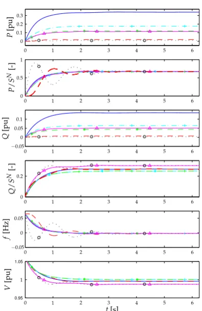
The simulation results in Fig. 2 show that all trajectories synchronize in less than 3 s. Condition (19) is satisfied, which indicates that the condition is robust – to a certain extent – to the presence of transfer and load conduc-tances. As predicted by Lemma 5.2, the active power is shared proportionally by the droop–controlled sources. The voltage amplitudes satisfy the typical requirement of 0.9 < Vs
i < 1.1 for Vis in pu and i∼n.¯ However, the
reactive power sharing among all units is not proportional. The observation that the stability condition (19) is, to a certain extent, robust to the presence of model uncertain-ties is reconfirmed in numerous further simulation scenar-ios with a large variety of different parameter settings.
7. CONCLUSIONS
0.95 1.05
P
[p
u
]
P
/
S
N
[-]
Q
[p
u
]
Q
/
S
N
[-]
f
[H
z]
V
[p
u
]
t[s] 0
0
0 0
0 0
0 0
0 0
0
1
1 1 1 1 1
1 1
2 2 2 2 2 2
3 3 3 3 3 3
4 4 4 4 4 4
5 5 5 5 5 5
6 6 6 6 6 6
−0.05 −0.05
0.05 0.05 0.1 0.1
0.2 0.2 0.3
[image:8.595.66.264.65.369.2]0.5
Fig. 2. Trajectories of the power outputsPi, Qi in pu, the
relative power outputs Pi/SiN, Qi/SNi , the internal
relative frequencies fi= (ωi−ωd)/(2π) in Hz and
the voltage amplitudesVi in RMS of the controllable
sources in the microgrid given in Fig. 1. The lines correspond to: battery 5b, i = 1 ’–’, FC 5c, i = 2 ’- -’, FC CHP 9b,i= 3 ’+-’, FC CHP 9c,i= 4 ’* -’, battery 10b,i= 5 ’△-’ and FC 10c,i= 6 ’o-’.
gains and setpoints of the voltage droop controllers, but does neither depend on the choices of the controller gains and setpoints of the frequency droop controllers nor on the low pass filter time constants. A design criterion on the controller gains and setpoints guaranteeing a desired steady–state active power distribution has been provided. The robustness of the stability condition with respect to model uncertainties, such as the presence of conductances, has been evaluated in a simulation example based on the CIGRE benchmark MV distribution network. The simula-tions show that the derived stability condition is satisfied and a desired steady–state active power distribution is achieved for a wide selection of different control gains, set-points, low pass filter time constants and initial conditions. Since droop control fails in general to achieve a desired reactive power distribution, future research concerns al-ternative, possibly distributed, solutions to this problem.
Appendix A. DEFINITION OF THE MATRICESD,L,˜ L,W ANDT(θS)
The matrix Dis given by
D:= diag
c
2m
kQm(V
s m)2
= diag
Vd
m+kQmQ
d m
kQm(V
s m)2
, m∼n.¯
(A.1) The entries of the matrices ˜L,L,WandT(θs) are given by
˜ lpp:=
n X
q=1
|Bpq|VpsV s q cos(δ
s
pq),˜lpq:=−|Bpq|VpsV s q cos(δ
s pq),
lii:= n X
q=1
|Biq|VisV s q cos(θ
s
iq), lik:=−|Bik|VisV s k cos(θ
s ik),
wii:= n X
q=1
|Biq|Vqssin(θ s
iq), wiq:=|Biq|Vissin(θ s iq),
tpp:=|Bpp|, tpq:=−|Bpq|cos(θspq), (A.2)
wherei∼n¯\ {n}, k∼n¯\ {n},as well asp∼n¯ andq∼n.¯ REFERENCES
Chandorkar, M., Divan, D., and Adapa, R. (1993). Control of parallel connected inverters in standalone AC supply systems. IEEE Trans. on Ind. Appl., 29(1), 136 –143. Coelho, E., Cortizo, P., and Garcia, P. (2002).
Small-signal stability for parallel-connected inverters in stand-alone AC supply systems. IEEE Trans. on Industry
Applications, 38(2), 533 –542.
Davy, R.J. and Hiskens, I.A. (1997). Lyapunov functions for multimachine power systems with dynamic loads.
IEEE Trans. on Circuits and Systems I, 44(9), 796–812.
Engler, A. (2005). Applicability of droops in low voltage grids.Int. Journal of Distr. Energy Resources, 1(1), 1–6. Guerrero, J., Loh, P., Chandorkar, M., and Lee, T. (2013). Advanced control architectures for intelligent microgrids – part I: Decentralized and hierarchical control. IEEE
Trans. on Industrial Electronics, 60(4), 1254–1262.
Kundur, P. (1994). Power system stability and control. McGraw-Hill.
Lasseter, R. (2002). Microgrids. InIEEE Power
Engineer-ing Society Winter MeetEngineer-ing, volume 1, 305 – 308.
Lopes, J., Moreira, C., and Madureira, A. (2006). Defin-ing control strategies for microgrids islanded operation.
IEEE Trans. on Power Systems, 21(2), 916 – 924.
Ortega, R., van der Schaft, A., Maschke, B., and Escobar, G. (2002). Interconnection and damping assignment passivity-based control of port-controlled Hamiltonian systems. Automatica, 38(4), 585–596.
Pogaku, N., Prodanovic, M., and Green, T. (2007). Mod-eling, analysis and testing of autonomous operation of an inverter-based microgrid. IEEE Trans. on Power
Electronics, 22(2), 613 –625.
Rudion, K., Orths, A., Styczynski, Z., and Strunz, K. (2006). Design of benchmark of medium voltage dis-tribution network for investigation of DG integration.
InIEEE PESGM, 6 pp.
Schiffer, J., Anta, A., Trung, T.D., Raisch, J., and Sezi, T. (2012). On power sharing and stability in autonomous inverter-based microgrids. In Proc. 51st IEEE CDC. Maui, HI, USA.
Schiffer, J., Goldin, D., Raisch, J., and Sezi, T. (2013). Synchronization of droop-controlled microgrids with dis-tributed rotational and electronic generation. InProc.
52nd IEEE CDC. Florence, Italy.
Schiffer, J., Ortega, R., Astolfi, A., Raisch, J., and Sezi, T. (2014). Conditions for stability of droop–controlled inverter–based microgrids. Automatica. Accepted. Simpson-Porco, J.W., D¨orfler, F., and Bullo, F. (2013a).
Synchronization and power sharing for droop-controlled inverters in islanded microgrids. Automatica, 49(9), 2603 – 2611.
Simpson-Porco, J.W., D¨orfler, F., and Bullo, F. (2013b). Voltage stabilization in microgrids using quadratic droop control. InProc. 52nd IEEE CDC. Florence, Italy. van der Schaft, A. (2000). L2-Gain and Passivity
Tech-niques in Nonlinear Control. Springer.