Probabilty hypothesis density filtering for real-time traffic state estimation and prediction

This is a repository copy of

Probabilty hypothesis density filtering for real-time traffic state

estimation and prediction

.

White Rose Research Online URL for this paper:

http://eprints.whiterose.ac.uk/82265/

Version: Submitted Version

Article:

Canaud, M., Mihaylova, L., Sau, J. et al. (1 more author) (2013) Probabilty hypothesis

density filtering for real-time traffic state estimation and prediction. Networks and

Heterogeneous Media (NHM), 8 (3). 825 - 842. ISSN 1556-1801

https://doi.org/10.3934/nhm.2013.8.825

[email protected] https://eprints.whiterose.ac.uk/

Reuse

Unless indicated otherwise, fulltext items are protected by copyright with all rights reserved. The copyright exception in section 29 of the Copyright, Designs and Patents Act 1988 allows the making of a single copy solely for the purpose of non-commercial research or private study within the limits of fair dealing. The publisher or other rights-holder may allow further reproduction and re-use of this version - refer to the White Rose Research Online record for this item. Where records identify the publisher as the copyright holder, users can verify any specific terms of use on the publisher’s website.

Takedown

If you consider content in White Rose Research Online to be in breach of UK law, please notify us by

VolumeX_{, Number}0X_{, XX}200X _pp.X–XX

PROBABILITY HYPOTHESIS DENSITY FILTERING FOR REAL-TIME TRAFFIC STATE ESTIMATION AND PREDICTION

Matthieu Canaud∗_{, Lyudmila Mihaylova}∗∗_{, Jacques Sau}∗ _{and Nour-Eddin El Faouzi}∗_♮

∗_{Universit´e de Lyon, F-69000, Lyon, France}

IFSTTAR, LICIT, F-69500, Bron, France ENTPE, LICIT, F-69518, Vaulx en Velin, France

∗∗_{School of Computing and Communications}

InfoLab21, South Drive, Lancaster University Lancaster LA1 4WA, United Kingdom

♮Smart Transport Research Center, Faculty of Build Environment and Engineering, Queensland University of Technology, Australia

Email: [email protected], [email protected], [email protected] Email: [email protected], Corresponding author

Abstract. The probability hypothesis density (PHD) methodology is widely used by the research community for the purposes of multiple object tracking. This problem consists in the recursive state estimation of several targets by using the information coming from an observation process. The purpose of this paper is to investigate the potential of the PHD filters for real-time traffic state estimation. This investigation is based on a Cell Transmission Model (CTM) coupled with the PHD filter. It brings a novel tool to the state estimation problem and allows to estimate the densities in traffic networks in the presence of measurement origin uncertainty, detection uncertainty and noises. In this work, we compare the PHD filter performance with a particle filter (PF), both taking into account the measurement origin uncertainty and show that they can provide high accuracy in a traffic setting and real-time computational costs. The PHD filtering framework opens new research avenues and has the abilities to solve challenging problems of vehicular networks.

1. Introduction. Sensor data fusion and advanced estimation methods can pro-vide information about special events and hence improve the traffic conditions in Intelligent Transportation Systems (ITS). Sussman [38] emphasizes the fact that the full benefits of these systems cannot be realized without the ability to pre-dict the short-term traffic conditions. Hence, the short-term prepre-diction of traffic states plays a key role in various ITS applications such as Advanced Traffic Man-agement Systems. In this context, the prediction of traffic flow variables such as traffic volume, travel speed or travel time for a short time horizon (typically 5 up to 30 minutes) is of paramount importance. However, the increasing complexity, non-linearity and presence of various uncertainties (both in the measured data and

2000Mathematics Subject Classification. Primary: 58F15, 58F17; Secondary: 53C35.

Key words and phrases. Traffic control, Particle filter, Probability Hypothesis Density filter, Traffic state estimation, Sequential Monte Carlo methods.

The first author is supported by COST TU0702 Action grant (STSM).

models) are important factors affecting the traffic state prediction. Consequently, prediction methods based on deterministic assumptions are incapable to meet the accuracy needed in ITS applications.

To overcome these limitations, many non-deterministic estimation methods have been investigated [1]. Multiple objects generate multiple measurements which orig-inate either from the targets or from the environment (which is the so-called clutter noise). In this scope, our research is focused on developing a stochastic traffic modeling framework that enables estimation (filtering and prediction) of some traf-fic states such as traftraf-fic flow with high accuracy. The purpose of this work is to investigate the potential of the Probability Hypothesis Density (PHD) filters for real-time traffic state estimation. The dynamic evolution is based on a Cell Trans-mission Model (CTM) coupled with the PHD filter as an estimation engine. The CTM is well known in traffic modeling, however the use of the PHD filter in traffic engineering is new and it offers the possibility to estimate traffic network densities. For the problem of multiple-object tracking, the PHD filter has been intensively studied and used in the literature [24]. This problem consists in the recursive state estimation of several targets based on the information coming from an observation process. However, the PHD filter has not been applied yet to traffic estimation problems (such as to the travel time for example) except for one paper [2] in which the PHD filter performance is studied jointly with a constant velocity model for estimation of trajectories of individual cars. Our work, in contrast to [2], develops a PHD filter for traffic networks, combines the CTM with the PHD filter and validates its performance over simulated data based on real data, collected in France.

Our paper is the first work which shows that the PHD methodology has a poten-tial to solve problems for vehicular traffic systems. The novelty of this work is that it formulates the traffic problem within the PHD framework, gives a solution in the presence of clutter and presents comparative results with a particle filter taking into account the clutter in the measurements. The PHD method is very appealing be-cause it avoids the need of data association and deals with the measurement origin uncertainty in an efficient way.

The paper is organized as follows. Section 2 formulates the objectives of this work, introduces the traffic modeling framework and the main considered filtering methodologies, i.e. the particle and PHD filters. Section 3 describes the macroscopic traffic model considered. Section 4 describes in details the PHD filtering method. An overview of the PHD method is given and the proposed PHD algorithm for traffic state estimation is described. Section 5 describes briefly the PF in the presence of measurement origin uncertainty. This PF is compared with the PHD filter. Section 6 presents the real-world test site and set up of the PHD filter. The analysis of the results and a comparison with the particle filter is then described. The last section 7 discusses extensions of this work and further research about the PHD filter for traffic state estimation under changeable weather conditions and also with data with high level of clutter noise. Appendix Apresents the derivation of the PF likelihood in the presence of measurement origin uncertainty.

2. Objectives.

state vector estimates along a part of the road, based on past measurements on the system.

In signal processing, Kalman filters (KFs) [21], including Extended Kalman Fil-ters [43] and Unscented Kalman Filters [20] have been widely used. Regarding traffic control applications, the high non-linearity of the dynamic systems has given raise to a wealth of alternative methods among which Sequential Monte Carlo methods, known also as Particle Filters [10,1] have become very popular. Extended Kalman Filters (EKFs) in combination with a stochastic traffic model have been applied in Wang et al. [43] in order to carry out the traffic state estimation. The proper choice of traffic parameter values is crucial in such applications, as highlighted in [43]. In order to address the proper choice of traffic parameters, in [44] the real-time traffic flow parameters and states are jointly estimated with an EKF. Another sequential filter which has recently received a lot of attention is the Ensemble Kalman Filter (EnKF) [46,47]. The method was originally proposed as a stochastic (Monte Carlo) alternative to the deterministic EKF.

Particle filters (PFs) have also shown their potential to solve the challenging traffic state estimation problems [27, 28]. In [3], [6], and [33] is demonstrated that particle filters can deal with the diverse meteorological traffic conditions. The promising results have demonstrated the accuracy of Sequential Monte Carlo meth-ods, which do not require any linearization. Moreover, the constant increase of the computational power has boosted their relevance to traffic state estimation. For instance, numerically efficient, parallel implementations of particle filters are pro-posed in [29]. However, new methodologies need to be explored, such as the one investigated in this paper i.e. the PHD filter and its highly attractive properties.

2.2. The Probability Hypothesis Density Filter. The PHD filter provides an elegant way to recursively estimate the number and the states of multiple targets given a set of observations. It works by propagating in time the first moment (called intensity function or PHD function) associated with the multi-target posterior [23]. Multi-target tracking is a common problem with many applications. The literature in this area is spread and the state-of-art and methodology are summarized well in [24,42]. Nevertheless, only one article is concerned with traffic modeling issues [2].

In [19] and [30] the authors highlight the fact that the PHD filter outperforms the standard approaches such as the KF or the Particle Filter (PF), especially in the way the measurement origin uncertainty is dealt with. The PHD filter is typically implemented either via the sequential Monte Carlo (SMC) method [39, 45] or by using finite Gaussian mixtures (GM) [40,41]. The GM method is attractive because it provides a closed-form algebraic solution to the PHD filtering equation, with the state estimate (and its covariance) easily accomplished. However, the GM method is based on somewhat restrictive assumptions that single-object transitional densities and likelihood functions are Gaussian, and that the probability of survival and the probability of detection are constant [24],[40]. The SMC method does not impose such restrictions and therefore provides a more general framework for the PHD filtering [35,48].

first implementations is introduced in [39]. Then some improvements have been proposed in [32] and [34].

Figure 1. The concept of PHD filtering, [24]

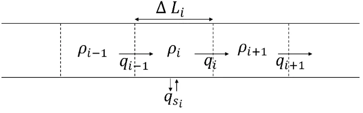
3. Macroscopic traffic model. The traffic model used is the Daganzo’s sending-receiving cell version of the Lighthill-Whitham-Richards (LWR) model [7], which is based on hydrodynamic analogy describing the behavior of the traffic flow. This model is classically written in a discrete version (as shown on Figure2) at a section level. The motorway section is divided intoncells of length ∆Li. The cell densities,

ρi for celli, and flows, qi for flow between cell i andi+ 1, are updated every ∆N

time interval. From the space discretization, a classical Godunov scheme is applied whose solution approximates the entropy solution [22].

Figure 2. Space discretization

The straightforward Godunov scheme consists of the two following equations:

ρi(k+ ∆N) =ρi(k) +_∆∆_LN

i qi−1(k)−qi(k)

, qi(k) = min Γi(k),Σi+1(k)

The first equation is the conservation equation. The second equation is the flow equation which consists of the demand-supply competitions, i.e. the resulting flow in celliat discrete timekwill be the minimum between celli+1 supply Σi+1(k) and

the cellidemand Γi(k). Note that the Stochastic Cell Transmission Model (SCTM)

developed by Sumalee et al., [36], extends the CTM to consider both supply and demand uncertainty. The numerical time step is taken as a sub-multiple of the observation time step fulfilling numerical conditions.

The state vector (of length 2n+ 1) to be estimated consists of the flows and densities in thencells of the section:

xk = ρ1(k), . . . , ρn(k), q0(k), . . . , qn(k)

T

, (2)

whereT _{denotes the transpose operator.}

The inputs uk of the system are the demand upstream and the supply

down-stream of the considered section. The state equation is then written as follows:

xk+1=f(xk, uk), (3)

where f is a complex and highly nonlinear function with no straightforward ana-lytical form.

For the traffic systems, the state equation (3) is commonly completed by a linear observation equation, which maps measurements, yk, and the state vector of the

system:

yk =Cxk, (4)

where C is a real matrix consisting of rows whose elements are all zero except for the element corresponding to the position of the sensor delivering a measurement. Note that this observation equation is not restricted to any constraint of linearity and could be choose nonlinear.

As there are uncertainties in both the measurements and the model, the complete traffic dynamical model is given by

xk=f(xk−1, uk−1) +wk,

yk =Cxk+vk, (5)

where wk andvk are zero mean Gaussian noises with respective variance matrices

Qk andRk.

4. PHD filtering.

4.1. General formulation. This section introduces the general formulation of the PHD filter for multiple targets. In this context target states and measurements are considered as random sets (random in values and also in number of values). From time step to time step, some of the targets may disappear. The surviving targets evolve to their new states and new targets may appear. Due to imperfections in the detector, some of the surviving and newborn objects may not be detected, whereas the observation setYk may include false alarm detections.

Suppose that at timekthere arenttarget states ˜x1,k, . . . ,x˜nt,keach taking value

in a state spaceχ ⊆Rn (n= dim x) and mk observations Yk ={y1,k, . . . , ymk,k}.

Within the PHD framework one can recursively estimate the state vector xk =

{x1˜ ,k, . . . ,x˜nt,k}of states of all nttargets given Y

of the PHD filter is to propagate a suitable density function D(x)abbr.= D(x|Y(k)₎ in the target stateχ.

The PHD is a density function but not a probability density function, such that, for any regionS⊆χ, the expected number of targets inS is given by

n(S) =

Z

S

D(s)dx, (6)

for a suitable density functionD(x).

Let’sD(·) be the PHD function andDk|k be the PHD function at timekbased

on the setY(k)_{of measurements till time instantk. The objective of the PHD filter} is the time propagation

Dk−1|k−1(x)→Dk|k−1(x)→Dk|k(x). (7)

Before presenting the predictor and corrector equations, we introduce some as-sumptions and notations. The PHD filter presumes some multi-target motion model. More precisely, target motions are statistically independent. Targets can disappear from the scene and new targets can appear independently of existing targets. These possibilities are described as follows.

• Motion of individual targets: fk+1|k(x|x′) is the single target Markov

transi-tion density.

• Probability of surviving: pS,k+1|k(x′) noted pS(x′) is the probability that a

target with statex′ _{at time stepk will survive in time stepk+ 1.}

• Appearance of completely new targets: bk+1|k(X) is the probability that new

targets with state setX will enter the scene at time stepk+ 1.

Note that in the general framework, new targets can be spawned by existing targets. In this case, we defined the spawning of new target by existing targets as bk+1|k(x|x′). However, in our context, this assumption could not be included

compared to the general PHD recursion [24] since it does not have any realistic sense.

The PHD filter also presumes the standard multi-target measurement model. More precisely, no target generates more than one measurement and each mea-surement is generated by no more than a single target, clutter meamea-surements are conditionally independent of the target state, missed detections, and a multi-object Poisson false alarm process. These assumptions can be summarized as follows:

• Single-target measurement generation: Lk(y|x) is the sensor likelihood

func-tion for observafunc-tiony at time stepkand statex.

• Probability of detection: pd,k+1|k(x′) noted pD(x′) is the probability that an

observation will be collected at time stepk+ 1 from a target with statex, if the sensor has statex′ _{at that time step.}

• False alarm density: At time stepk+ 1, the sensor collects an average number λ = λk+1(x) of Poisson-distributed false alarms, the spatial distribution of

which is governed by the probability densityc(y).

With these notations, we now describe the basic steps of the PHD filter, each in turn: initialization, prediction and correction.

1. PHD Filter initialization

2. PHD Filter predictor

At time stepk, starting fromDk|k, the predictive PHDDk+1|k can be

calcu-lated [23] in the following way:

Dk+1|k(x) = bk+1|k(x)

| {z }

birth targets +

Z

Fk+1|k(x|x′)Dk|k(x′)dx′, (8)

where the PHD “pseudo-Markov transition density” is Fk+1|k(x|x′) =pS(x′)fk+1|k(x|x′)

| {z }

persisting targets

+bk+1|k(x|x′)

| {z }

spawned target

, (9)

with the spawned target equal to zero in our study case. The predicted number of targets is therefore

Nk+1|k =

Z

Dk+1|k(x)dx. (10)

Then we have, under the non-restrictive assumption of no spawning,

Dk+1|k(x) =bk+1|k(x) +

Z

pS(x′)fk+1|k(x|x′)Dk|k(x′)dx′. (11)

3. PHD Filter corrector

From the previous step, one has the predicted PHDDk+1|k(x), given by (11).

At time step k+ 1, one collects a new observation set Yk+1 ={y1, . . . , ym}

and can calculate the data updated PHD Dk+1|k+1(x). The PHD corrector

step is [23]:

Dk+1|k+1(x) =Lk+1(y|x)Dk+1|k(x), (12)

where the “PHD pseudo-likelihood” function is defined by

Lk+1(y|x) = 1−pD(x) +pD(x)

X

y∈Y

Lk(y|x)

λc(y) +R pD(x′)Lk(y|x′)Dk+1(x′)dx′

(13)

Then we have,

Dk+1|k+1(x) = [1−pD(x)]Dk+1|k(x) +

X

y∈Y

pD(x)Lk(y|x)Dk+1|k(x)

λc(y) +R pD(x′)Lk(y|x′)Dk+1(x′)dx′

.

(14) 4.2. SMC-PHD algorithm for traffic state estimation. Due to the highly nonlinear traffic model, we choose the SMC implementation for the approximate propagation of the traffic PHD. At each time stepkthe PHDDk|k is approximate

by a set of particles and associated weights, {(xi, wi)} Np

i=1. The integral over this intensity is the estimated expected number of targets and it is not necessarily equal to one. The SMC-PHD algorithm is composed of three main steps: (i) a prediction step with the newborn generation and propagation via the traffic model; (ii) a correction step in which particle weights are updated through the likelihood function and the new measurements set; and (iii) a resampling step from the existing one with an update of the weights. More precisely, at time step k, the algorithm is as follow:

1. Step 1: Prediction Let{xi, wi}

Np

to avoid a large number of additional particles since the state space is high dimensional. Hence, the newborn particles set is drawn from the distribution

N(yk−1, Q), i.e. centered around the previous step measurement yk−1 with the measurement covarianceQ. The corresponding weights are equal to 1/Nb,

withNb the number of born particles.

Then, we sample particles xi at time step k from those of time step k−

1 according to the traffic model, weights being unchanged, and we define

{˜xi, wi} Np+Nb

i=1 as the predicted particle set containing the newborn and per-sisting particles.

2. Step 2: Correction

For the new particle set and new mk measurements, we compute the

likeli-hoodLk(yk|x) according to (˜ 13). Then the respective covariance matrices are

calculated for each estimated state ˆy by

˜ C(j) =

Np X

i=1 wi

h

(Cx˜i−yˆj) (Cx˜i−yˆj)T

i

, j= 1. . . mk. (15)

This matrix ˜Ccharacterizes the particle distribution of the state ˆy. Finally, we update the target intensity, given the new measurements through a correction of the individual weights. For every particle of set{x˜i, wi}

Np+Nb

i=1 :

ˆ wi =

mk X

j=1

wipD(˜xi)Lk(yj,k|x˜i)

˜

C(j) . (16)

3. Step 3: Resampling From the particle set{x˜i, wi}

Np+Nb

i=1 , randomly select a particle set of length Np and rescale the weights to get the new particle set for the next step. Note

that, any standard resampling technique for particle filtering can be used. The next section describes the PF framework and the PF likelihood expression when taking into account the clutter noise for traffic estimation.

5. A particle filter taking into account the clutter noise for traffic esti-mation. In the case of multiple targets, multiple measurements are generated and there is measurement origin uncertainty. Some of these measurements are not from the targets, but instead from clutter. In order to compare the developed PHD filter with a PF under the same conditions, the PF takes into account the clutter in the measurements too. This is done by calculating the likelihood of the PF as sug-gested in [13,14]. It is assumed that the number of measurements and the number of clutter points have a Poisson distribution.

The PF is a Monte Carlo approach which gives a numerical solution for the prediction

p(xk|y1:k−1) = Z

Rnx

p(xk|xk−1)p(xk−1|y1:k−1)dxk−1 (17)

and respectively for the measurement update equation

p(xk|y1:k) =

p(yk|xk)p(xk|y1:k−1)

p(yk|y1:k−1)

, (18)

pdf, p(xk|y1:k) is the posterior state pdf at time step k, p(yk|xk) is the likelihood

function andp(yk|y1:k−1) is a normalization factor.

The PF approximates the posterior state pdfp(xk|y1:k) by means of a collection of

Npparticles and their respective weights{x

(i)

k , w

(i)

k } Np

i=1. After the arrival of the new measurements the weights are updated according to the likelihood functionp(yk|xk).

The cloud of particles evolves with time and depending on the observations, so that the particles represent with sufficient accuracy the pdf of the state.

At each time step a set of sensor measurements is recorded. These measurements could come from either targets or clutter. The basic idea is to figure out how to assigns each measurement to the right target or identify it as a false alarm.

In the context of PF multiple-target tracking the data association problem can be resolved as proposed in [13] and [14]. Similarly to [13] we have derived the expression for the PF likelihood for the traffic estimation problem

p(Yk|x

(i)

k )∝ mk Y

j=1

λCpC(yjk) +λTpT(yjk|x

(i)

k )

, (19)

where λT is the mean value of the number of measurements originated from

the targets, λC is the mean value of the number of measurements corresponding

to clutter, with Yk being the set yjk, j = 1, . . . , mk of measurements at time

k, pT(yjk|x

(i)

k ) and pC(yjk) are respectively the target and clutter measurement

likelihood defined by a single Gaussian for target measurements and by a uniform distribution for the clutter [14]. Note that the pC is independent of the target.

Appendix A presents the derivation of the PF likelihood for the considered traffic estimation problem. The next section presents results showing the performance of the two algorithms.

6. Performance evaluation.

6.1. Site and collected data. The test site is the urban freeway in Eastern part of Lyon’s ring road (point A to D on figure3), which consists of three lanes between km point A and km point B (5.6km long), [4,33]. Traffic data were provided by the urban motorways’ operator CORALY and collected in 2007 from 8 loop sensors. The length of each cell is, respectively: 1080, 480, 1200, 840 750, 780 and 480 meters.

A rainy day’s upstream demand and downstream supply and balances of ramp movements was used. The profiles of these external actions on the motorway system come from the real data of highway flow measurements in March 2007, on one week-day (Tuesweek-day). The motorway section under consideration is the most frequently congested part. The upstream flow comprises the flow from North-West Lyon and the on-ramp from the Geneva freeway (point B). Therefore, the upstream demand presents high values on classical peak hours in the morning and at the end of the afternoon.

Figure 3. Test site section (B →C) divided into 7 cells and its detector configuration

6.2. Hypotheses, model and filter parameters. From previous works, e.g. [33], it is known that for this test site under rainy conditions (which is the case of the selected day), the fundamental diagram of the LWR model is well represented with the following parameters:

1. Critical density: ρc=100 [veh/km];

2. Maximum density: ρM=300 [veh/km];

3. Maximum flow: qM=138 [veh/min].

The respective variance matrices of the estimation algorithms are chosen as fol-lows. For the flow measurement uncertainty the standard deviation is σR=1.5

[veh/min] (consistent with the empirical analysis conducted on the raw data col-lected on this network). Hence, the measurement noise variance matrix is defined as a diagonal matrix: Rt=diag(σ2R). Regarding the uncertainty of the state

equa-tion, we assume that the model is as robust as the measurements, meaning that the standard deviation of the state vector flow part is the same as measurements one (σQ=1.5 [veh/min]). The density magnitudes are much smaller than those giving

the flow; therefore the standard deviation of the density part of the state vector is chosen to be:

σk =σQ×

ρc

qM

= 0.0011 [veh/m]. (20)

Thus, thenfirst diagonal elements of theQmatrix are equal toσ2

k whereas the

(n+ 1) last ones are equal to σ2

Q.

We choose the following parameters in the filters’ implementation: 1. Probability of detection: Pd=0.98;

2. Number of particles: Np=100;

3. Number of newborns: Nb=250;

4. Mean of clutter intensity (false alarm): λT=1.

The PHD value D0|0 is initialized with uniformly distributed particles which corresponds to lack of prior knowledge. Moreover, as the newborn object particles need to cover the entire state-space with reasonable density for the PHD filter, the birth density is driven by measurements following a uniform distribution as suggested in [32].

6.3. Performance evaluation. The developed PHD filter for real-time traffic state estimation is evaluated by a comparison with the PF with likelihood func-tion taking into account the clutter noise as derived in the Appendix A, similarly to [13,14]. The two filters are implemented under the same conditions (filter and model parameters). Finally, we compare the flow estimates obtained from both filters and for each sensor location.

Simulations have been conducted with a laptop having 4 GB RAM and an Intel i3-2330M 4.20GHz processor. The CPU times of the two algorithms implemented in Matlab are measured for the whole considered period. Both approaches give similar results, around 20 seconds for the whole time interval, which could be considered as a proof of their applicability in real time.

for both estimation methods (see Figure5). The Root Mean Square Error (RMSE)

RM SEi=

1 NsNt

Ns X

j=1

Nt X

k=1 ˆ

yi,j(k)−yj(k)

2

(21)

is used as a measure of the performance. The subscript i = PF or PHD, Ns is

the number of sensors, Nt is the number of time steps and ˆyi,j(k) the traffic flow

estimates for respective filteri, sensorj at timek.

Since with real data, the noises are unknown, the process has been conducted one simulated data with a determined level of noises. The difference ˆy−yshows the error in percentage and then we can see the performance for all filters with respect to the ground truth data. The model used to simulate data is the same as the one used in the filters in which the level of noises of the simulated data is defined by the diagonal ofQ.

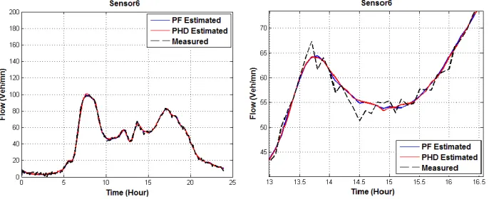
Figure 5. Actual versus estimated flows for cell 6 (left) and zoom (right). Dot-lines represent real measured flows and blue and red solid line are respectively PF and PHD estimates

As one can see, with only boundary conditions given to the filters, the accuracy of the state estimates provided by the PHD filter and PF is quite similar, and close to the actual measurements with a noticeable PF better accuracy. The respective RMSEs are: RM SEP F=1.63 [veh/min] andRM SEP HD=2.23 [veh/min].

However, the PHD estimates appear smoother than those given by the PF, which can be an interesting feature if one looks at the confidence interval of estimates. Hence, in our case, the PHD filter performed as well as the PF and the trend of the differences between RM SEP F and RM SEP HD is the same as it can be seen

from Figure5. Table1summarizes the results at each sensor location. One can see that the accuracy of the state estimates of the PHD and PF are comparable. It is important to note the overestimation of the PHD compared with the PF, mainly due to the smoother characteristics.

cell 1 cell 2 cell 3 cell 4 sensor sensor sensor sensor RM SEP F 1.32 1.76 1.84 1.85

RM SEP HD 1.18 2.14 2.45 2.78

cell 5 cell 6 cell 7 cell 8 sensor sensor sensor sensor RM SEP F 1.82 1.86 1.72 0.86

RM SEP HD 2.78 2.57 2.71 1.22

Table 1. RMSE, [veh/min] of the flow estimates with simulated data

The RMSE boxplot explicitly demonstrates a general lower value for PF estima-tion compared to the PHD filter. This last one is also more spread. Nevertheless, both mean values are small, which represents a close estimation of the ground truth. Regarding at CPU time boxplot, one can see a tight distribution and most of all real-time applications appear relevant since for the applied methods the mean values are almost equal to 20 seconds for the whole period of the study.

Figure 6. Boxplot of RMSE (left) and CPU Time (right)

7. Conclusions and perspectives. This paper develops a Probabilistic Hypoth-esis Density filter for traffic state estimation. The PHD filter is implemented based on a Sequential Monte Carlo algorithm. Its performance is evaluated over simu-lated data based on a real-world study case. The results obtained are compared with the PF, known for its ability in solving traffic state estimation problems as well as prediction.

is relevant in multi-target multi-source tracking. One can consider urban traffic and the estimation of other information such as travel time under various noise uncertainties.

The Cardinalized PHD filter framework [26] is an extension of the PHD filter and we aim at developing CPHD filters for the vehicular traffic problems. The Cardinalized PHD filter propagates not only the first moment but also the second order moment and estimates the number of targets. The Box Particle filter [15,16,

17,34] is another promising approach that can deal with various uncertainties and can be applied to vehicular traffic estimation, also in combination with the PHD filter. Both approaches can be useful in the attempt of defining some metrics of the travel time, for example metrics such as reliability or consistency.

In conclusion, this first work on PHD filtering for traffic estimation shows its rel-evancy. Based on the analogy with PF, the use of PHD filter for prediction appears suitable. However, some special features have to be investigated as the likelihood function, the calibration of some parameters while the assimilation process: clutter law and parameters like rate, resampling improvement, detection profile and so on. Nevertheless, this filter has a great interest and definitively need more consideration since it can be potentially useful for many traffic applications.

Our work opens doors to next investigations for traffic prediction which will be with cardinality PHD filters (including for joint state and parameter estimation) and other PHD techniques. This work can be extended to solve traffic filtering and prediction problems with different weather conditions.

Acknowledgments. This work is part of the COST action TU0702 research ac-tivities: “Real-time Monitoring, Surveillance and Control of Road Networks under Adverse Weather Conditions” [11]. The authors would like to thank CORALY (Lyons urban motorways managers) for providing them with data. We would like to acknowledge also the UK Engineering and Physical Sciences Research Council (EPSRC) for the support via the BTaRoT grant EP/K021516/1 and the European Commission Marie Curie programme “OPTIMUM” for the support provided to this study in the form of International Research Staff Exchange Scheme (IRSES) Cooperation Research Program - www.optimum-project.net.

REFERENCES

[1] M. Arulampalam, S. Maskell, N. Gordon and T. Clapp, A tutorial on particle filters for online nonlinear/non-Gaussian Bayesian tracking, IEEE Transactions on Signal Processing, 50_{, 174–188 (2002).}

[2] G. Battistelli, L. Chisci, S. Morrocchi, F. Papi, A. Benavoli, A. Di Lallo, A. Farina and A. Graziano,Traffic intensity estimation via PHD filtering, In Proc. 5th European Radar Conf., Amsterdam, The Netherlands, 340-343, (2008).

[3] A. Ben Aissa, J. Sau, N-E. El Faouzi and O. De Mouzon, Sequential Monte Carlo Traffic Estimation for Intelligent Transportation System: Motorway Travel Time Prediction Appli-cation, In Proc. of the 2nd ISTS, Lausanne, Switzerland (2006).

[4] R. Billot, N-E. El Faouzi, J. Sau and F. De Vuyst,Integrating the impact of rain into traffic management: online traffic state estimation using sequential Monte Carlo techniques, In Transportation Research Records (2010).

[5] Z. Chen, Bayesian filtering: From Kalman filters to particle filters, and beyond, Adaptive Systems Lab., Technical Report, McMaster University, ON, Canada (2003).

[7] C. Daganzo,The cell transmission model: A dynamic representation of highway traffic con-sistent with the hydrodynamic theory, Transportation Research B,28, 269–287 (1994). [8] A. Doucet,Monte Carlo methods for Bayesian estimation of hidden Markov models.

Appli-cation to radiation signals, PhD thesis, Universit Paris-Sud, Orsay (1997).

[9] A. Doucet, On sequential simulation-based methods for Bayesian filtering, Departement of Engineering, Technical report CUED/F-INFENG/TR.310, Cambridge University (1998). [10] A. Doucet, N. De Freitas and N. Gordon, Sequential Monte Carlo Methods in Practice,

Springer (2001).

[11] N-E. El Faouzi,Research Needs for Real Time Monitoring, Surveillance and Control of Road Networks under Adverse Weather Conditions, Research Agenda for the European Coopera-tion in the field of scientific and technical research (COST), (2007) - www.COST-TU0702.org. [12] O. Erdinc, P. Willett, and Y. Bar-Shalom, Probability hypothesis density filter for multi-target multisensor tracking, In Proc. of the 8th Int. Conf. on Information Fusion, 146-153, Philadelphia, PA, USA (2005).

[13] K. Gilholm, S. Godsill, S. Maskell and D. Salmond,Poisson models for extended target and group tracking, In Proc. SPIE: Signal and Data Processing of Small Targets 5913, 230-241, San. Diego, CA, USA (2005).

[14] K. Gilholm and D. Salmond,Spatial distribution model for tracking extended objects, In Proc. IEEE on Radar, Sonar and Navigation,152, 364 - 371, (2005).

[15] A. Gning, L. Mihaylova and F. Abdallah,Mixture of uniform probability density functions for non linear state estimation using interval analysis, In Proc. of the 13th Int. Conf. on Information Fusion, Edinburgh, UK (2010).

[16] A. Gning, B. Ristic and L. Mihaylova,A box particle filter for stochastic set-theoretic mea-surements with association uncertainty, In Proc. of the 14th Int. Conf. on Information on Fusion, Chicago, IL, USA (2011).

[17] A. Gning, B. Ristic and L. Mihaylova, Bernouilli particle/box particle filters for detection and tracking in the presence of triple uncertainty, IEEE Trans. Signal Processing,60_{, 2138} -2151, (2012).

[18] A. Hegyi, D. Girimonte, R. Babuska and B. De Schutter,A comparison of filter configurations for freeway traffic state estimation, In Proc. of the 2006 IEEE Intelligent Transportation Systems Conference (ITSC 2006), 1029 - 1034, Toronto, Canada (2006).

[19] R. Juang and P. Burlina,Comparative performance evaluation of GM-PHD filter in clutter, In Proc. of the 12t Internatiinal Conf. on Information Fusion, 1195 - 1202, (2009).

[20] S. Julier and J. Uhlmann, A new extension of the Kalman filter to nonlinear systems, In International Symposium on Aerospace/Defense Sensing, Simulation and Controls, 182–193, Orlando, FL, USA (1997).

[21] R. Kalman, A new approach to linear filtering and prediction problems, Journal of Basic Engineering,82, 35–45 (1960).

[22] J. Lebacque, The Godunov scheme and what it means for first order traffic flow models, In Proc. of the 13th nternaional symposium on transportation and traffic theory (ISTTT), 647-677, (1995).

[23] R. Mahler,Multitarget Bayes filtering via First-order Multitarget Moments, IEEE Transac-tions on Aerospace and Electronic Systems,39_{, 1152–1178 (2003).}

[24] R. Mahler,Statistical multisources multitarget information fusion, Artech House, 2007. [25] R. Mahler, PHD filters for nonstandard targets, I: Extended targets, In Proc. of the 12th

International Conference on Information Fusion, 914–921, Seattle, WA, USA (2009). [26] R. Mahler, B-T. Vo and B-N. Vo,CPHD Filtering With Unknown Clutter Rate and Detection

Profile, IEEE Transactions on Signal Processing,59_{, 3497–3513 (2011).}

[27] L. Mihaylova and R. Boel,A particle filter for freeway traffic estimation, In Proc. of the 43rd IEEE Conference on Decision and Control,2, 2106-2111, Atlantis, Paradise Island, Bahamas (2004).

[28] L. Mihaylova, R. Boel and A. Hegyi,Freeway Traffic Estimation within Recursive Bayesian Framework, Automatica,43(12), 290–300 (2007).

[29] L. Mihaylova, A. Hegyi, A. Gning and R. Boel, Parallelized Particle and Gaussian Sum Parti-cle Filters for Large Scale Traffic Systems,IEEE Transactions on Intelligent Transportation Systems. Special Issue on Emergent Cooperative Technologies in Intelligent Transp. Systems, 13(1), 36 - 48, (2012).

[31] B. Ristic, M. Arulampalam and N. Gordon,,Beyond the Kalman Filter: Particle Filters for Tracking Applications, Artech House, Boston (2004).

[32] B. Ristic, D. Clark and B. Vo,,Improved SMC implementation of the PHD filter, In Proc. of the 13th International Conference on Information Fusion, Edinburgh, UK (2010).

[33] J. Sau, N-E. El Faouzi and O. De Mouzon,Particle-filter traffic state estimation and sequen-tial test for real-time traffic sensor diagnosis, In Proc. of ISTS’08 Symposium, Queensland (2008).

[34] M. Schikora, A. Gning, L. Mihaylova, D. Cremers and W. Koch,Box-Particle PHD Filter for Multi-Target Tracking, IEEE Trans. on Aerospace and Electronic Systems, to appear (2013). [35] H. Sidenbladh,Multi-target particle filtering for the probability hypothesis density, In Proc.

6th Int’l Conf. on Information Fusion, Cairns, Australia (2003).

[36] A. Sumalee, R.X. Zhong, T.L. Pan, and W.Y. Szeto, Stochastic cell transmission model (SCTM): a stochastic dynamic traffic model for traffic state surveillance and assignment, Transportation Research Part B,45, 507–533 (2011).

[37] X. Sun, L. Munoz and R. Horowitz,Highway traffic state estimation using improved mixture Kalman filters for effective ramp metering control, In Proc. of th 42nd IEEE Conf. on Decision and Control, 6333-6338, Maui, Hawaii, USA (2003).

[38] J. Sussman,Introduction to Transportation Problems, Artech House, Norwood, Masachussets, 2000.

[39] B. Vo, S. Singh and A. Doucet,Sequential Monte Carlo methods for multi-target filtering with random finite sets, IEEE Trans. Aerospace and Electronic Systems,41, 1224–1245 (2005). [40] B. Vo and W. Ma,The Gaussian mixture probability hypothesis density filter, IEEE Trans.

Signal Processing,54, 4091–4104 (2006).

[41] B-T. Vo, B-N. Vo and A. Cantoni,Analytic implementations of the cardinalized probability hypothesis density filter, IEEE Trans. Signal. Processing,55_{, 3553–3567 (2007).}

[42] N.-N. Vo, B.-T. Vo, and D. Clark, Bayesian Multiple Target Tracking Using Random Finite Sets, Ch. 3 in Integrated Tracking, Classification, and Sensor Management: Theory and Applications, Eds. M. Mallick, V. Krishnamurthy, and B.-N. Vo, 75-125. John Wiley & Sons, 2012.

[43] Y. Wang, M. Papageorgiou and A. Messmer,Real-time freeway traffic state estimation based on extended Kalman filter: A case study, Transportation Science,41_{, 167–181 (2007).} [44] Y. Wang, M. Papageorgiou, A. Messmer, P. Coppola, A. Tzimitsi and A. Nuzzolo,An adaptive

freeway traffic state estimator, Automatica,45, 10-24 (2009).

[45] N. Whiteley, S. Singh and S. Godsill, Auxiliary particle implementation of the probability hypothesis density filter, IEEE Trans. on Aerospace and Electronic Systems, 46, 1437-1454 (2010).

[46] D. Work, S. Blandin, O-P. Tossavainen, B. Piccoli, and A. Bayen, A distributed highway velocity model for traffic state reconstruction, Applied Mathematics Research eXpress,2010, 1-35 (2010).

[47] D. Work, O.-P. Tossavainen, S. Blandin, A. M. Bayen, T. Iwuchukwu and K. Tracton, An ensemble Kalman filtering approach to highway traffic estimation using GPS enabled mobile devices, Proceedings of CDC, 5062-5068, (2008).

[48] T. Zajic and R. Mahler,Particle-systems implementation of the PHD multitarget tracking filter, In Proceedings of SPIE, Signal Processing, Sensor Fusion, and Target Recognition, XII, Vol. 5096, 291-299, Bellingham (2003).

Appendix A. Likelihood derivation of the Particle Filter. We shall start from expression (11) of the article of Gilhom and Salmond (GS) [14], adapting the notations to our ones. With no loss of generality we shall omit here the time in-dex k, the set of measurements at time k being denoted asY ={y1, y2, . . . , ym}.

The likelihood function is then written, separating explicitly the product part re-lated to φ(j) 6= 0(target measurements) from the one related to φ(j) = 0(clutter measurements):

p(Y|x)∝X

φ

(λT/λC)nT(φ) m

Y

j,φ(j)6=0

pT(yj|x) m

Y

j,φ(j)=0

The definition of φ (partitions of the set {1,2, ...., m}), nT(φ) (number of target

measurements) compatible with partitionφ,nC(φ) =m−nT(φ) (number of clutter

measurements) are the same as in [14].

In the previous expression, the first product involvesnT factors and the second

nC. The previous expression (22) is multiplied byλmC, leading to:

p(Y|x)∝X

φ m

Y

j,φ(j)6=0 aj

m

Y

j,φ(j)=0

bj (23)

with:

aj = λTpT(yj|x)

bj = λCpC(yj). (24)

We can use here the same procedures as the Appendix of the GS paper. We define all possible assignments φ as Φ0,Φ1. . . ,Φm, where Φi is the set of all mappings

that assignimeasurements to the target, i.e. those withnT(φ) =i. Relation (23)

can be rewritten in the form:

p(Y|x)∝

m

X

i=0



X

φ∈Φi

m

Y

j,φ(j)6=0 aj

m

Y

j,φ(j)=0 bj



. (25)

In the bracket of the previous expression (25), the first product involvesi factors and the secondm−i factors. The sum on Φi, which scans all the mappings with

i objects chosen among m ones, involves then m!/(i!(m−i)!) terms. The total number of terms in expression (25) is then 2m_.

Let us consider now the product:

A=

m

Y

j=1

(aj+bj) = m

Y

j=1

Aj (26)

The development of the previous product, can be ordered in the following way: first, for an integeri(0≤i≤m), we add all the possibilities of products ofifactorsajs

chosen among them Ajs andm−ifactorsbjs taken from the remainingm−i Ajs.

This gives exactly the sum on Φi of relation (25). Second, summing forifrom 0 to

m gives the likelihood expression of equation (25). The product giving A is then exactly the likelihood expression (25). We get then:

p(Y|x)∝

m

Y

j=1

(λCpC(yj) +λTpT(yj|x)) (27)

where we have used the definition (24) of theajs andbjs.

A meaningful physical interpretation of the previous expression can be easily given. The previous likelihood is the product of effective elementary likelihoods, each of them being a weighted mixture of clutter and target original ones. It is clearly seen how clutters can blur the result by the relative magnitude of the clutter term compared with the target one, for which it can be noted the contribution of the clutter creation rate versus the target creation rate.

E-mail address:[email protected]

E-mail address:[email protected]

E-mail address:[email protected]