On the assessment of passive devices for structural control via real-time dynamic substructuring

This is a repository copy of On the assessment of passive devices for structural control via real-time dynamic substructuring.

White Rose Research Online URL for this paper: http://eprints.whiterose.ac.uk/80971/

Version: Submitted Version

Article:

Londo no, J.M., Serino, G., Wagg, D.J. et al. (2 more authors) (Submitted: 2012) On the assessment of passive devices for structural control via real-time dynamic substructuring. Structural Control and Health Monitoring, 19 (8). 701 - 722. ISSN 1545-2255

https://doi.org/10.1002/stc.464

Reuse

Unless indicated otherwise, fulltext items are protected by copyright with all rights reserved. The copyright exception in section 29 of the Copyright, Designs and Patents Act 1988 allows the making of a single copy solely for the purpose of non-commercial research or private study within the limits of fair dealing. The publisher or other rights-holder may allow further reproduction and re-use of this version - refer to the White Rose Research Online record for this item. Where records identify the publisher as the copyright holder, users can verify any specific terms of use on the publisher’s website.

Takedown

If you consider content in White Rose Research Online to be in breach of UK law, please notify us by

On the assessment of passive devices for structural

control via Real–Time Dynamic Substructuring

Juli´an M. Londo˜noa,∗

, Giorgio Serinoa_{, David J. Wagg}b_{, Simon A. Neild}b_,

Adam J. Creweb

a

Department of Structural Engineering, University of Naples Federico II, 80125 Naples, Italy

b

Faculty of Engineering, University of Bristol, Queens Building, University Walk, Bristol BS8 1TR, UK

Abstract

In this work the applicability of a dynamic testing technique known as Real– Time Dynamic Substructuring (RTDS) for the assessment of passive control systems in seismic protection of buildings is analysed. RTDS is an efficient method for the assessment of dynamic and rate–dependent behavior of sys-tems subjected to dynamic excitation at real scale and in real scenarios. To guarantee the validity and accuracy of a RTDS simulation, a stability analysis of the substructured system should be completed. In this paper we present explicit analyses which provide a dynamic characterization of the delay–induced phenomena in RTDS tests when considering passive control systems with strong nonlinearities. We present a complete set of closed–form expression to describe the main phenomena due to the delay in terms of dy-namic stability in a RTDS simulation. Through an experimental study we confirm the existence of self–sustained oscillations. Those were caused by very small delays in the feedback loop, which unavoidably lead the system to instability as a result of the high frequency oscillations.

Keywords: Delayed systems, Piecewise smooth dynamical systems, Substructuring testing

∗_{Corresponding author}

Email addresses: [email protected](Juli´an M. Londo˜no),

1. Introduction

Reducing the response of buildings or bridges to strong earthquakes is of great concern for structural engineers in preventing large damage or col-lapse. The application of structural control technologies for protection of civil structures has been growing in interest over the last four decades, not only to reduce the response under extreme dynamic loads but also to in-crease the system reliability and provide human comfort during everyday environmental loads [1]. The response of structures under strong dynamic loads is highly unpredictable and then difficult to model, it becomes even more complex when designing infrastructures which include some kind of anti–vibration systems.

General nonlinear numerical models are non–suitable for describing the dynamic behavior of buildings incorporating energy dissipators because the main structure is supposed to remain elastic while the non–linearities are left to dissipators. In addition, the coexistence of elements with extremely

different stiffness parameters1 _{could lead to numerical instability and to a}

certain lack of accuracy. Seeking for better understanding of the behavior of complex structural systems under strong dynamical loading, different lab-oratory facilities and experimental methodologies have been developed for years (e.g. [2, 3]). However, the vast majority of those techniques suffer from technical and physical limitations that restrict their applicability for assess-ing real scenarios. Major problems are related to: (i) physical limitations for large scale structures such as bridges and buildings; and (ii) challenging experimental issues like the reproduction of hysteresis and rate–dependent phenomena (See e.g. [4, 5]).

We are interested in the experimental assessment of passive control sys-tems for seismic protection of buildings. We will exploit a state of the art of the dynamic testing technique known as Real–Time Dynamic Substruc-turing (RTDS) [6], for the assessment of passive systems in real scenarios. RTDS testing is an efficient method for the assessment of dynamic and rate– dependent behavior of systems subjected to dynamic excitation. It provides the capability to isolate and physically test critical components of a

struc-1_{Dissipators can be significantly more flexible than the main structure and the bracing}

ture whilst the remaining part of it is simulated numerically. Tests can be conduced at real scale and in real time to fully capture any rate dependency, while allowing for hundreds of repeatable tests [7].

On of the first reported RTDS was performed on a viscous damper located at the base of a multi–storey building [8]. Therein only the damper was tested physically while the building was modelled as a linear single degree of freedom (SDOF) system. A real–time test using a linear SDOF numerical substructure was also performed in [9], with the physical test specimen being a stiffness, damping or inertia element.

The concept of pseudodynamic testing has been successfully extended to real–time scales for testing nonlinear structures as in [10], and for testing velocity–dependent components as in [11] and [12]. As well, some experi-ments on RTDS have been carried out by using shaking table facilities. For instance, in [13] a large structural mass of the single DOF system is separated into two parts: the smaller part selected as the experimental substructure and the larger one (with attached spring and dashpot) as the numerical sub-structure to conduct a test in the shaking table. Similarly in [14], the upper part of a building is chosen as the experimental substructure and the lower part is considered as the numerical one to perform a RTDS test by using a shaking table facility. In [15] a substructure shaking table test is performed to reproduce large floor responses of high–rise buildings at full–scale.

An interesting result is also presented in [16], where a RTDS test of a he-licopter rotor blade coupled with a lag damper is conducted to produce a realistic representation of the dynamic characteristics of the overall blade system. In addition, RTDS test has also been used for testing semi–active control devices. Recently in [17] a test for three large–scale MR fluid dampers simulating the seismic response of a three–storey steel frame structure was presented. A technique called virtual coupling was used to ensure an appro-priate tradeoff between performance and stability.

In this paper we present two explicit analyses which provide a dynamic characterization of the delay–induced phenomena in RTDS tests when con-sidering passive control systems with strong nonlinearities. We present a complete set of closed–form expression to describe the main phenomena due to the delay in terms of dynamic stability in a RTDS simulation. We could identify not only the region where harmful self–sustained high frequency os-cillations arise but also the limit cycle induced. Through an experimental study on RTDS testing, we confirm the existence of such a self–sustained oscillations. These were caused by very small delays in the feedback loop, which unavoidably lead the system to instability as a result of high frequency oscillations.

This paper is organized as follows. Section 2 presents some fundamen-tals of RTDS testing; Section 4 shows the proposed compensation scheme base on adaptive filters; whilst section 4 is devoted to the explicit analyses where delay effects are described mathematically. The case study and some experimental results are presented in Section 5, whereas the final remarks and conclusion are discussed in Section 6.

2. Real–Time Dynamic Substructuring Testing

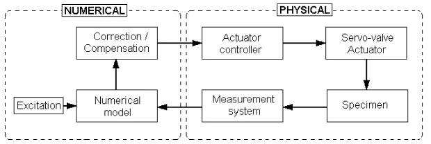
An RTDS simulation is a hybrid method involving a physically tested part and a numerically modelled part. The most critical part of the sys-tem is selected and extracted to be tested in the laboratory physically. The two substructures are complementary to form the complete emulated struc-ture. During RTDS simulations, the physical substructure interacts with a computational model (numerical substructure) by means of a feedback loop; both substructures send and receive data to each other, because they need to know the state of the other part to work out their own. Figure 1 shows a block diagram of a substructuring test. In a typical displacement controlled test, the displacements of the degrees of freedom of interest are calculated

using the numerical model and are passed to the delay compensator. The

corrected signal is in turn passed to the actuator controller. The controller

generates signals to drive theactuators which impose these displacements on

the specimen while the forces required to impose them are detected by the

measurement system and passed back to the numerical model. The transfer system is typically a single (electric or hydraulic) actuator with its controller, but may also be a more complex test facility like a shaking table.

ex-Figure 1: Block diagram of a substructured system.

change information in real time with minimum error between them. Each subsystem in the above scheme requires some time for performing its own task. As a consequence of this fact, the feedback signal arrives with some de-lay to the numerical model. Although such dede-lay comes from the cumulative time lags of each subsystem, the main contribution comes from the actuator. The success of real–time substructuring tests is then highly dependent on the

performance of the actuators2_{, whose imperfect dynamics can introduce both}

timing and amplitude errors into the signal. These can affect the accuracy of the performance of the test [18]. To overcome this, time delay compensation schemes have been commonly used to make corrections on the actuator com-mand signal. For instance, in [19] the use of simple polynomial curve fitting was investigated; therein stable and accurate results were achieved in a RTDS simulation by using a third–order polynomial. As well, the effectiveness of the extrapolation and interpolation procedures was evidenced in [20] through a series of substructuring tests applied to a multi degree of freedom (MDOF) structure. Also in [21] an adaptive forward prediction algorithm based on compensation by polynomial extrapolation was presents; the methodology is flexible, accurate and able to be applied to multi–actuator environments. Even if the compensation scheme is well suited and works properly, it becomes impossible to reduce the transport delay to zero. So that, the sensitivity of the whole substructured system to delays should be estimated.

2

3. Delay compensation by adaptive filters

Delay in command signals is a serious issue for dynamic systems which need to work in real time. It is essential for the stability and accuracy of a RTDS simulation to make corrections to the signals being transmitted between numerical and physical substructures, as otherwise errors may cu-mulate during the test and make it unreliable. Delay compensation is a well known technique with the most common strategy being delay compen-sation by extrapolation and Smith predictor [22]. It is a common practice to approximate the time delay on command signal as constant. Although this is not strictly correct, it can be considered a reasonable approximation at the relatively low frequencies normally encountered in Civil Engineering dynamics [23]. In this work we tried an alternative compensation scheme. The compensated command signal is generated by the prediction forward of the current command signal by using an adaptive filter. It is autonomously adjusted each time step by using the data available. This method provides a robust prediction criterion against noisy data. It proved to be both accurate and faster than common methodologies in prediction.

3.1. Forward prediction scheme

An adaptive filter can be thought of as a digital filter that performs signal processing and adapts its performance based on the input signal. The filter

coefficients, w, are adjusted to minimize the mean–square error between its

output, d(n), and that of an unknown system, y(n), (LMS algorithm). To

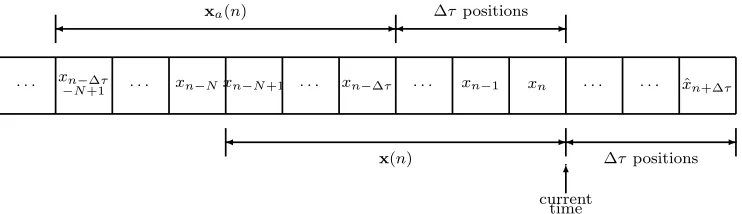
set up the filter for forward prediction, we take advantage of the available data at the current time step. The data are arranged into two buffers for

both adapting and predicting. Thus, the predicted point ˆx is estimated as a

linear function of previous samples as:

ˆ

x(n+ ∆τ) = xT(n)w(n) (1)

where x(n)=_{x(n), x(n₋1), x(n₋2), . . . , x(n₋N + 1)_}, x(_·) are the

dis-crete samples of the signal to be predicted, n the current time step, N is

the filter order and ∆τ is the number of time steps required to match the

time delay τ3_{. To update the filter coefficients, we evaluate the filter}

perfor-mance in predicting the last known point of the signal, that is x(n). So, we

considered the instant error e(n) as:

e(n) =d(n)−y(n) (2)

Herein the desired output y(n)=x(n), and the filter output is calculated by:

d(n) =xT_a(n)w(n) (3)

wherexa(n)={x(n−∆τ), x(n−∆τ −1), . . . , x(n−∆τ −N + 1)}is the data

buffer for adapting. The filter coefficients can be then updated by using

for-mula (4) where µ is the learning rate (0 < µ < 1). It was derived from

gradient based optimization considering the square error as the cost function (For details see [24, Ch.6]).

w(n+ 1) = (1−µ)w(n) + 2µe(n)xT(n) (4)

· · · xn₋∆τ

−N+1 · · · xn−Nxn₋N+1 · · · xn₋∆τ · · · xn₋1 xn · · · xˆn+∆τ

-

-x_{(n) ∆τpositions}

xa(n) ∆τpositions

6

current time

Figure 2: Data buffer for the prediction scheme.

This prediction scheme based on adaptive filters have proved a high gen-eralization capacity and tolerance to noisy data. Unlike common method-ologies, it is able to smooth out the effects of noise and experimental errors avoiding slight discontinuities in the predicted signal. A discussion of this and some comparative examples including common prediction methodologies can be found in [25].

4. Delay and stability

thus, the system could become unstable and develop oscillations exponen-tially increasing in amplitude as was shown by Wallace et al in [26]. In what follows, we present both a linear and nonlinear explicit analyses where delay effects are described mathematically.

4.1. Explicit stability analysis – Linear damper

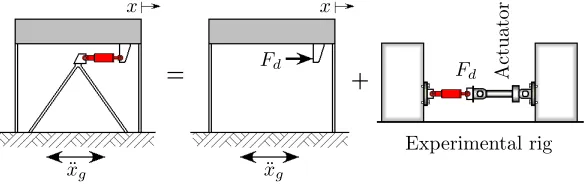
Let us consider a single degree of freedom system (SDOF) with an added linear viscous fluid damper as shown in Figure 3. We assume the damper as the critical component of the structural system. Consequently, the damper becomes the physical substructure and is extracted from the system to be tested in the lab at real scale. We also suppose a displacement–controlled real–time substructuring simulation, which means that the displacements

computed through the numerical model (SDOF system + damper force Fd)

are applied through an actuator to the specimen (the damper), and in turn, the damper resisting force is measured and fed back into the numerical sub-structure. To represent the substructured system under this configuration, a constant transport delay is included in the damper response.

Assuming that the damper reaction force is linear with respect to the

x

Fd

c k

m −mx¨g

x m

Damper

¨

xg

Figure 3: Single degree of freedom oscillator with an added damper.

x x

Fd _F

d

¨

xg x¨g

Ac

tu

at

or

Experimental rig

velocity, Fd=cdx˙, the system dynamics can then be written as:

mx¨(t) +cx˙(t) +kx(t) +cdx˙(t−τ) =−mx¨g(t) (5)

where m, is the mass of the system; c, is the intrinsical damping coefficient

of the system; k, is the stiffness of the system;t andτ, are respectively time

and the signal delay; cd, is the damping coefficient of the damper; ¨xg, is the

base excitation; and ¨x,x, x˙ , are respectively the system acceleration, velocity

and displacement.

Let us consider zero external excitation and an arbitrary initial condition. The system in (5) can be rewritten with non–dimensionalized parameters as:

d2_x dˆt2 + 2ζ

dx

dtˆ+x+p dx

dˆt tˆ−τˆ

= 0 (6)

where:

wn = r

k

m ; ζ =

c

2√mk ; ˆt =wnt ; τˆ=wnτ ; p=

cd

mwn

Following the standard practice, we assume solutions of the form x =Aeλˆt_.

Thus, the characteristic equation of the system can be written as:

λ2+ 2ζλ+ 1 +λpe−λτˆ _{= 0 (7)}

To determine the stability boundaries of the system, we can search for a set of points in the parameters space where the characteristic equation has one pair of pure imaginary roots, that is, just go through a Hopf bifurcation [27].

To find this curve, we substitute into the trial solution λ = iwˆ, for w > 0

and ˆw=w/wn. After applying this substitution, equation (7) becomes:

−wˆ2 + 2iζwˆ+ 1 +ipweˆ −iwˆˆτ _{= 0 (8)}

Applying the Euler’s formula from complex analysis and splitting up into real and imaginary parts, we get two real equations:

−wˆ2+pwˆsin( ˆwτˆ) + 1 = 0 (9)

2ζ+pcos( ˆwτˆ) = 0 (10)

Assuming ζ as known, we can use the last pair of equations to express the

parameters ˆτ and pas function of ˆw.

ˆ

w2₋₁

−2ζwˆ = tan( ˆwτˆ) ⇒ τˆ=

1 ˆ

warctan

1−wˆ2

2ζwˆ

+nπ

ˆ

w ; n = 1,2,3. . .

wheren corresponds to then-th lobe (parameterized by ˆw) from the right in

the stability diagrams in Figure 5 (n must be greater than 0, because ˆτ > 0).

The trigonometric terms in Equations (9) and (10) can be eliminated by squaring and adding them to yield:

p= 1

ˆ

w

p

( ˆw2₋₁₎2_{+ (2ζwˆ)}2 ₍₁₂₎

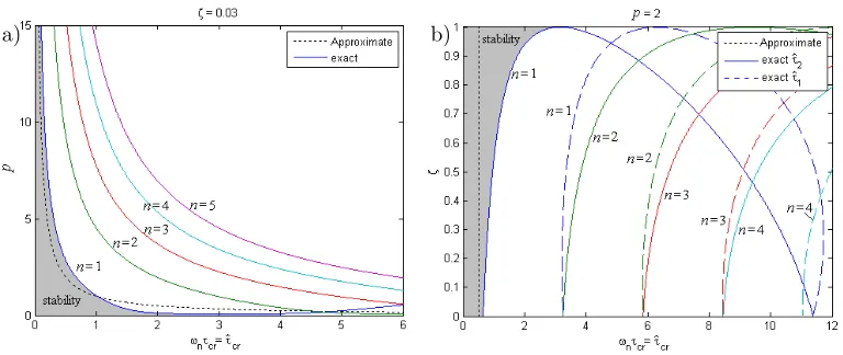
In Figure 5(a), we present the boundaries obtained for ˆτ and p by fixing ζ

at 0.03. These curves are parameterized by ˆw running from 0 to ∞ and n

from 1 to 5. Along these curves the system has a pair of purely imaginary eigenvalues delimiting the parameters space where the system is expected to be stable.

We can also rearrange equations (9) and (10) assuming p as known. Thus,

we obtain the critical delay ˆτ and ζ as parametric curves in ˆw:

ζ = 1

2 ˆw

p

(pwˆ)2_{−( ˆw}2₋₁₎2 ₍₁₃₎

ˆ

τ1 = 1 ˆ

warcsin

ˆ

w2−1

pwˆ

+ 2πn

ˆ

w (14)

ˆ

τ2 =₋1 ˆ

w

arcsin

ˆ

w2₋₁ pwˆ

+π

+2πn

ˆ

w (15)

where ˆwruns from 1₂(−p+pp2_{+ 4) to} 1

2(p+

p

p2_{+ 4), andn is any positive}

integer greater than zero. Figure 5(b) shows the stability region for fixed

p = 2 using the curves defined parametrically by equations (13), (14) and

(15). Considering the lightly damped systems commonly studied in civil

engineering applications (ζ < 0.1), the curve ˆτ2 with n = 1 can be used

as the practical stability boundary because encloses the others theoretical boundaries into the unstable region.

Any system lying in the stability region (grey zone) is well-behaved and so, the results from the substructuring test represent in a fitting manner the dynamics of the whole original system. It is worthy noticing that for a linear damper there exist always a stability region, i.e., we can establish a critical delay below which the stability in the RTDS simulation would be guarantee. Also note that for larger dampers the stability margin is narrow; this implies

that when testing large dampers (p greater), even a very short delay could

a) b)

Figure 5: Non–dimensionalized complex root solutions: a) Varying added damper capacity, and b) Varying structural damping.

4.2. Explicit stability analysis – Nonlinear damper

Let us consider an added nonlinear viscous fluid damper with constant delay in the single degree of freedom system shown in Figure 3. The delay differential equation (DDE) for that system can be written as:

mx¨+cx˙ +kx+cd|x˙(t−τ)|α·sign( ˙x(t−τ)) =−mx¨g (16)

where α is the non–linear exponent of the damper (0< α <1); _{| · |}represents

the absolute value of · ; and the other parameters as described before for

equation (5).

Again, let us consider zero external excitation, arbitrary initial conditions and some appropriate substitutions to get a formulation in terms of the following dimensionless parameters. Thus, after some algebra we have:

z′′

(ˆt) + 2ζz′

(ˆt) +z(ˆt) +pn|z

′

(ˆt₋ˆτ)_|α

·sign z′

(ˆt₋τˆ)

= 0 (17)

where:

ζ = c

2√mk; τˆ=wnτ; wn=

r

k

m; x=x0z; pn=

cd

mw

α−2

n |x0| α−1

The differentiating operator ′

indicates the derivative with respect to ˆt, and

Nonlinear dampers with lower exponent have more energy dissipation capacity than those with higher exponent. That is why nonlinear fluid devices

with lowαare very appreciated for real applications in structural engineering,

as they provide significantly higher forces at lower velocities compared to linear dampers and more energy dissipation capacity [28]. According with exhaustive numerical simulation, systems equipped with nonlinear damper at low damper’s velocity exponents have qualitatively equivalent dynamics. We call two systems equivalent if their phase spaces have the same dimension, the same number and type of invariant sets, in the same general position with respect to each other (See Fig 8). Hence, when analysing stability of

systems with added nonlinear dampers with lowα, let sayα≤0.20, we could

consider a dynamically equivalent model fixing α=0; that is, a model which

uses dry friction (Coulomb friction) instead of viscous nonlinear damping. This will not compromise the general result of the stability analysis.

Thus, we can rewrite the model to be analysed as:

z′′(ˆt) + 2ζz′(ˆt) +z(ˆt) +pssign z

′

(ˆt−τˆ)

= 0 (18)

where the damper force is represented bypssign(z

′

(ˆt−τˆ));ps =cd/(mx0w2n).

In turn, this model can be represented in terms of the equations of state by

substituting x1 =z and x2 =z′

to yield:

x′

1(ˆt) = x2(ˆt)

x′

2(ˆt) = −2ζx2(ˆt)−x1(ˆt)−pssign x2(ˆt−τˆ)

(19)

The idea is to use a simpler mathematical model, in such a way that the explicit analysis can be achieved in a closed–form. The advantage in this change lies in the fact that such a system can be modelled by a piecewise linear set of ODEs of the form:

Ψτˆ :x

′

=Ax+Bu (20)

where x _{∈ R}2 is the two–dimensional state vector; A and B are the system

matrices in controllable canonical form as presented in (21), and the switching

parameter u obeys the switching rule in equation (22).

A=

0 1

−1 −2ζ

; B =

0

−ps

(21)

u=

1.0

−1.0

if x2(ˆt₋τˆ)>0

if x2(ˆt−τˆ)<0

We term F1(x) the system vector field of Ψτˆ whenu= 1.0; F2(x) the vector

field of Ψτˆ when u = −1.0. In addition, we will label as φi(x0, t) the flow

generated by Fi (i= 1,2), such that:

d

dt(φi(x,ˆt)) = Fi(φi(x,ˆt)); φi(x0,0) =x0 (23)

Note that the system’s evolution in time is uniquely determined once we

have defined the values of x1, x2, and u. Thus, in the three–dimensional

space (x1, x2, u), we can visualise the state space as two parallel half–planes,

partially overlapping wherever u can have two different values for the same

pair (x1, x2).

4.2.1. Delay by changing the switching rule

The main idea behind the use of piecewise smooth dynamical systems is to reap the benefits of including, in a very easy way, the effects of the delay in the system dynamics. Thus, after some proper transformations, we can study the stability of an equivalent non–delayed system, rather than focusing on a complex delayed system (Further information in [29]).

Without loss of generality, we will focus our attention on trajectories

gen-erated by the vector field F1 along its valid domain. The flow φ1 can be

obtained by solving (20) with u=1.0 giving:

φ1(x0,ˆt) =

a1eλ1ˆt_+a2eλ2ˆt−_p

s

a1λ1eλ1tˆ_+a2λ2eλ2ˆt

(24)

wherex0 = (x10, x20) is the initial condition,λ1,2are the eigenvalues of matrix

A and:

a1 =Cλ(x20−(x10+ps)λ2) ; a2 =Cλ(−x20+ (x10+ps)λ1) ; Cλ =

1

λ1₋λ2

The above expressions allows us to calculate the trajectory of the system in

(18) on the (x1, x2)–plane from any initial condition underF1. Similarly, the

flow φ2 can be obtained by solving (20) with u=−1.

Now consider the dynamics of system (20), note that the delay ˆτ is only

explicit in the switching rule. Let us suppose ˆτ = 0 and label the boundaries

where x2 changes sign as:

Σ+₁₂ := {x_∈R2 :x1 >−ps, x2 = 0}

Σ−

Note that Σ+₁₂ is the subset where the switching condition is satisfied for

changing from F1 to F2, whilst Σ−₁₂ is the subset where is satisfied for going

back from F2 toF1. Henceforth, they will be referred as switching sets.

To introduce the effects of the delay in the system dynamics, observe

that if a trajectory crosses one of the switching sets Σ+₁₂ or Σ−₁₂, because of

the delay, the actual switching from one system configuration to the other

will occur after some time defined by ˆτ. Indeed, switchings occur on the

delayed switching sets Στˆ+

12 and Στˆ

−

12 which are images of Σ+12 and Σ

−

12 under

the system flow φi for some time delay. Specifically we have,

Σˆτ+

12 := {φ1(x,τˆ), x∈Σ+12}

Σˆτ12−:= {φ2(x,τˆ), x∈Σ

−

12}

(26)

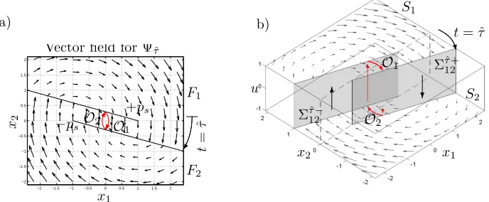
The original switching sets rotate clockwise around the corresponding point

−2 −1.5 −1 −0.5 0 0.5 1 1.5 2 −2

−1.5 −1 −0.5 0 0.5 1 1.5 2

x1

x2

Vector field for Ψτˆ

a)

F1

F2

−ps

+ps

t

=

ˆ

τ

O2

O1

ˆ

τ

b)

x2 x1

u

Στˆ+ 12

Στˆ−

12

S1

S2

? 6

Wt= ˆτ

O2

O1

Figure 6: Vector fields of the piecewise linear system Ψτˆ in (20) for ˆτ = 0.4,ζ = 0.03,

ps= 1.0: a) (x1, x2)–plane; b) three–dimensional space (x1, x2, u).

(0,-psu) as shown in Figure 6. The position of Σˆτ12+ in the (x1, x2)–plane can

be easily determined by computingφ1 for any initial condition falling on Σ+₁₂

and t= ˆτ. Similar procedure can be done for Στ₁₂ˆ−by consideringφ2 and Σ−₁₂.

Therefore, instead of analysing the delayed model, we can replace the system in (20) by a non–delayed system which includes the dynamic effects of the de-lay by moving the original switching sets towards the corresponding dede-layed switching sets. Thus, we can rewrite the delayed system (20) as follows:

Ψ0 :x′ =Ax+Bu; u7→

1.0

−1.0

if x_∈Στˆ−

12

if x_∈Στˆ+

12

where the above switching rule establishes that, parameter u switch to 1.0

(or −1.0) only when the respective condition (27) is satisfied, that is to say,

when the trajectory hits Σˆτ12− (or Στˆ

−

12), and will remain fixed at this value

until condition (27) is again satisfied. This effect of the delay on the switch-ing rule, was firstly envisaged when studyswitch-ing the dynamics of a delayed relay feedback system [29]. In that work, the authors demonstrated that the dy-namics of the delayed system remain qualitatively the same as those of a

system with properly constructed switching sets. This is true for all ˆτ ≤ π,

what is expected for well–controlled experiments. For larger delays, the dy-namics become much more complicated and will not be considered here.

Two main unstable phenomena have been observed for the system with an added delayed nonlinear damper. We found that even the smallest de-lay causes self–sustaining oscillations in the system’s response, such kind of oscillation is well–known as limit cycle. The larger the delay, the longer the limit cycle. This limit cycle is characterized for oscillations at high fre-quency, much higher than the natural frequency of the system. In addition, there exists a region in the neighborhood of the limit cycle, where the system behaviour is altered drastically. When the states of the system get into this area (See Figure 8), the amplitude and frequency of the oscillations change suddenly. These oscillations tend to match the limit cycle; however, if delay is very small, such convergence is very slow in terms of displacements. This critical region is characterised for high frequency oscillations and only occurs

for small delays. When ˆτ becomes larger, the system goes rapidly to the

limit cycle without any other important vibratory phenomenon in between. In previous works, the authors have investigated analytically the exis-tence of both the limit cycle and the critical region of oscillations at high frequencies. In [30] a comprehensive analytical study is presented. From that document, we extract here just the main concerning results which cor-responds to closed-form expressions for describing the phenomena pointed out before.

The limit cycle exists and is symmetric since the following conditions are verified.

• No intersection exists between the delayed switching sets, i.e.,

Σˆτ12+∩Στˆ

−

12 =∅ (28)

with respect to the origin, i.e.,

φ1(x

∗

,ˆt∗

) = ₋x∗

for some x∗ _∈Στˆ−

12 (29)

φ2(−x∗,ˆt∗) = x∗

for some −x∗ _∈Στ12ˆ+ (30)

Due to the fact that even a small delay causes no intersection between the

switching sets Στˆ+

12 and Στˆ

−

12, any delay implies the existence of a limit cycle.

The explicit expression for calculating the evolution time required by an

oscillation under the limit cycle _O, that is the period of the limit cycle, can

be written as:

ˆ

T∗

= 2

λ1 ln

x∗

1(mΣ−λ2) +bΣ+psλ2

−x∗

1(mΣ−λ2)−bΣ +psλ2

(31)

where x∗ = (x∗

1, x

∗

2) is the point on the (x1,x2)–plane where the limit cycle

presents the maximum velocity. This point coincides with the state of the

system for which, under the limit cycle, the expression pssign x2(ˆt−τˆ)

changes sign. To find x1, we present also an equation which is implicit

function of x∗

1 and can be solved numerically (For further details see [30]).

x∗

1(mΣ −λ1) +bΣ+psλ1

−x∗

1(mΣ −λ1)−bΣ+psλ1

=

x∗

1(mΣ −λ2) +bΣ+psλ2

−x∗

1(mΣ −λ2)−bΣ+psλ2

λ 2 λ₁

(32)

where, in turn

mΣ =

φ12(xps,τˆ) φ11(xps,τˆ) +ps

; bΣ =−psmΣ (33)

and xps = (ps,0). The second–order subscript indicates the element position

inφ1 calculated for a flow underF1 with an evolution time equal to the delay

ˆ

τ.

Note that all the other variables in formulas (32) and (33) are known and easily derivable from the problem parameters through the expression pre-sented before. The maximum velocity developed under the limit cycle can be then calculated from:

x∗

2 =mΣx

∗

1+bΣ (34)

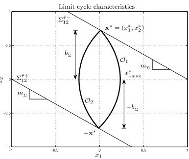
In the same way, the critical zone characterised by high frequency oscillations

can be defined by using four point in the (x1, x2)–plane, which enclose that

region. These point are (-ps,0), (x⋆1,x⋆2), (ps,0), (-x⋆1,-x⋆2), where:

x⋆

1 =

−bΣ(mΣ+ 2ζ)−ps

mΣ(mΣ + 2ζ) + 1

−1 −0.5 0 0.5 1 −1

−0.5 0 0.5 1

!"#$%

#&'($&*&+,-x1 x2

Σˆτ₋

12

Σˆτ+ 12

mΣ

mΣ x∗_{= (x}∗

1, x∗2)

−x∗

−bΣ bΣ

x∗

1max

O1

O2

Figure 7: Names of the characteristics in the limit cycle.

x⋆2 =mΣx

⋆

1+bΣ (36)

If the so-called high frequency zone exits, the condition (37) must be satis-fied, otherwise the system just goes rapidly to the limit cycle defined above without any other phenomenon arising.

−x⋆1 > x

∗

1 (37)

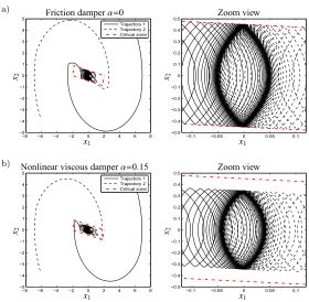
Figure 8 shows the phase planes of two arbitrary trajectories of the

sys-tem (27). We considered a SDOF syssys-tem with properties: mass m=1000Kg,

stiffness k=5×105_{N/m and damping ratioζ=3%. Also, we supposed a}

non-linear viscous fluid damper added to the system with exponent α=0.15 and

a nonlinear coefficient cd=50kN(sec/m)0.15. Figure 8a shows the trajectories

for a SDOF system with an added delayed friction damper (α=0 andps=2.0);

whilst Figure 8b shows the trajectories considering a SDOF system with the

added delayed nonlinear fluid viscous damper (α=0.15 and pn=2.03). We

also included in both cases the high frequency region which was delimited by

using the point x⋆_=(x⋆

1, x⋆2)=(-1.86, 0.87). Note how the trajectories of both

−8 −6 −4 −2 0 2 4 6 8 −5 −4 −3 −2 −1 0 1 2 3 4 5 Trajectory 1 Trajectory 2 Critical zone

−0.1 −0.05 0 0.05 0.1 −0.5 −0.4 −0.3 −0.2 −0.1 0 0.1 0.2 0.3 0.4 0.5 x₁ x₁ x2 x2

Friction damperα₌0 Zoom view

a)

−8 −6 −4 −2 0 2 4 6 8 −5 −4 −3 −2 −1 0 1 2 3 4 5 Trajectory 1 Trajectory 2 Critical zone

−0.1 −0.05 0 0.05 0.1 −0.5 −0.4 −0.3 −0.2 −0.1 0 0.1 0.2 0.3 0.4 0.5 x₁ x₁ x2 x2 Zoom view

Nonlinear viscous damperα₌0.15

b)

Figure 8: Phase plane of two arbitrary trajectories from numeric simulations for ζ=0.03 and ˆτ=0.224. a) Solution of the system in (18) for ps=2.0; b) Solution of the system in

(17) for α=0.15 and pn=2.03 .

be used to reach a reliable dynamic characterization of the SDOF system with a delayed nonlinear viscous fluid damper in a RTDS configuration. For the example, for the above parameters we have:

Peak limit cycle velocity, ˙x∗

=x∗

2x0wn = 0.505m/sec.

Peak damper force under the limit cycle, F∗

dmax = 50(0.505)

0.15 _{= 45.13kN.}

Period of oscillation under the limit cycle, T∗

= ˆT∗

/wn= 0.039sec.

These values can be compared against the data extracted from the numerical simulations. Note that the feedback signal in the RTDS configuration is the damper force and that is estimated with good accuracy.

Peak limit cycle velocity, 0.39m/sec.

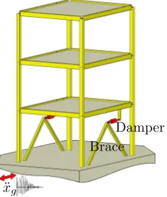
5. Case study

We considered a passive control system installed on a symmetric 3–storey one–bay steel framed building as shown in Figure 9. Two nonlinear viscous fluid dampers are placed on rigid braces at the first floor on opposite build-ing’s sides. We only considered one–directional base excitation along the axis where the dampers are placed. In order to set up the RTDS test, the

¨

xg

Damper Brace

Figure 9: Sketch of the passive controlled system analysed.

system is split up into two subsystems, keeping the dampers as the physi-cal substructure while the remains of the structure is modelled numeriphysi-cally. Also, in consequence of the symmetry from both the structural configura-tion and load, a RTDS which takes into account just one damper is enough to emulate properly the system, as long as due care is taken in the sub-systems’ interaction interface. Namely, the force fed back to the numerical substructure was twice the measured force from the physical substructure. A simplified lumped–mass model of the skeletal structure has been employed as the numerical substructure. We consider such a simple model because it is the fastest numerical substructure we can get. Once the delay issues are overcome, we can try more complete, complex and of course slower to com-pute numerical models. The dampers are included as a single external force applied to the first mass. It is updated in accordance with the measurements from the damper during the simulation.

The classical expression for describing this model is given by the ordinary

differential equation (ODE) in formula (38) where: M, K, C represent the

structural mass, stiffness and damping matrices; ¨xg(t) indicates the base

structural responses namely: displacement, velocity and acceleration,

respec-tively. The coefficients of the damping matrixChave been derived from those

of M and K imposing a mass and stiffness proportional damping (Rayleigh

damping) with modal damping ration equal to 3%.

MX¨(t) +CX˙(t) +KX(t) = −Mx¨g(t) +LU(t) (38)

being:

L=





0 0

−1 0 0 ₋1



, M= 



5430.2 0 0 0 5430.2 0 0 0 5430.2



 (Kg)

C=





9.817 −2.878 −0.625

−2.878 9.192 ₋3.508

−0.625 ₋3.504 6.313



×103(Nsec_m)

K=





12.091 ₋6.046 0

−6.046 12.091 −6.046 0 ₋6.046 6.046



×106 (_mN)

The dampers used in these tests (See Fig. 10) are characterized by a peak

force up to 50KN, stroke _±25mm and peak velocity about 0,3m/sec.

Figure 10: Non–linear viscous damper used in the tests.

Their constitutive force–velocity law may be described by means of

equa-tion (39) where ˙xd represents the relative velocity between the ends of the

damper in meters per second; cα is the nonlinear damping coefficient equal

to 60kN(sec

m)

0.15 _{and α is the velocity exponent equal 0.15.}

FD =cα|x˙d|αsign( ˙xd) (kN) (39)

5.1. Delay estimation and prediction.

Once the experimental rig was set up (see Figure 14), several tests were accomplished in order to measure the delay due to the actuator dynamics. The delay between the actual command signal (target displacement to be tracked for the actuator) and the current displacement signal (measured dis-placement) was estimated by using two different methodologies. Namely, (i)

zero crossing, in which the delay is estimated as the average of all of the

instantaneous delays measured when the time history crosses zero; andcross

correlation function which is a measure of similarity between two signals as a function of a time–lag applied to one of them, so it provides a overall delay estimation at the time–lag where the two signals are maximally corre-lated. Figure 11 shows the test time history, the synchronization plot and the force–displacement cycles when the command signal is a 2Hz sine wave with amplitude of 15mm. The delays estimated for several tests (using harmonic signal) are presented in Table 1.

2 2.5 3 3.5 4 4.5 5

−20 −10 0 10 20

Actual Displ (mm) Measured Displ (mm)

−20 −10 0 10 20

−20 −10 0 10 20

−20 −10 0 10 20

−50 0 50

D

is

p

la

ce

m

en

t

(m

m

)

Time (sec)

Sine wave test 2Hz at±15mm

Measured disp (mm)

M

ea

su

re

d

d

is

p

(m

m

)

Actual disp (mm) M

ea

su

re

d

fo

rc

e

(k

N

)

Figure 11: Sine wave test 2Hz at _±15mm: time history, synchronization plot and force-displacement cycles.

In light of the frequency range evaluated, the delays were estimated en-circling 15msec. Some sinusoidal sweep test were evaluated too. A wave

at _±10mm which speeds from 0.5Hz up to 4.0Hz in 5sec and goes back to

Amplitude Freq. Delay (msec)

(mm) (Hz) (X–corr) (zero–X)

1.0 -14 -18.90

5.0 -16 -15.27

10.0 0.5 -15 -13.76

15.0 -16 -16.83

20.0 -13 -14.19

1.0 -16 -15.02

5.0 -15 -15.01

10.0 1.0 -15 -14.52

15.0 -15 -14.91

20.0 -15 -15.23

1.0 -16 -14.01

5.0 -15 -14.49

10.0 2.0 -15 -14.99

15.0 -16 -15.98

20.0 -18 -19.63

5.0 -16 -15.75

10.0 3.0 -16 -16.32

15.0 -20 -20.47

(X-corr) Cross correlation function ; (zero-X) Zero crossing

Table 1: Delays estimated for sinusoidal wave form tests.

2 2.5 3 3.5 4 4.5 5 5.5 6 6.5

−10 −5 0 5

10 Actual Displ (mm)

Measured Displ (mm)

−10 −5 0 5 10

−10 −5 0 5 10

−10 −5 0 5 10

−50 0 50 D is p (m m ) Time (sec)

Sine sweep test at±_10mm

Measured disp (mm)

M ea su re d d is p (m m )

Actual disp (mm)

M ea su re d (k N ) a)

2 2.5 3 3.5 4 4.5 5 5.5 6 6.5

−0.01 0 0.01

2 2.5 3 3.5 4 4.5 5 5.5 6 6.5

−0.018 −0.016 −0.014

−18.50 −18 −17.5 −17 −16.5 −16 −15.5 −15 −14.5

5 10 Time (sec) D is p (m

) Time history

D el ay (s ec ) Delay (msec) H is to g ra m b)

Figure 12: a) Sine sweep test from 0.5Hz to 4.0Hz at_±10mm: time history, synchronization plot and force-displacement cycles. b) Delay estimation by zero crossing of the sinusoidal sweep test.

there exist different delays for the load and unload branches (which is more evident for higher frequencies), it may be due to the connection loose (back-lash behaviour) which incorporates an additional damper reaction delay.

In order to test the time delay compensation scheme based on adaptive filters, a predictor was set up to estimate the command signal 15msec for-ward. Some noise was added to the command signals to be predicted (SNR ratio=30dB). Figure 13 shows the tests run at University of Bristol after us-ing the time delay compensation scheme proposed. The coherence plot shows the scheme is able to compensate for delay even if noise is added. Also from

1.5 2 2.5 3 3.5 4 4.5

−20 −10 0 10 20

Actual Displ (mm) Predicted (mm) Measured Displ (mm)

−20 −10 0 10 20

−20 −10 0 10 20

−20 −10 0 10 20

−50 0 50 D is p (m m ) Time (sec)

Sine wave test 2Hz at±_15mm

Measured dis (mm)

M ea su re d d is (m m )

Actual disp (mm)

M ea su re d (k N ) a)

1.5 2 2.5 3 3.5 4 4.5 5 5.5

−10 −5 0 5 10

Actual Displ (mm) Predicted (mm) Measured Displ (mm)

−10 −5 0 5 10

−10 −5 0 5 10

−10 −5 0 5 10

−50 0 50 D is p (m m ) Time (sec)

Sine sweep test at±_10mm

Measured disp (mm)

M ea su re d d is p (m m )

Actual disp (mm)

M ea su re d (k N ) b)

Figure 13: Performance after using time compensation scheme. a) Sine wave test 2Hz at

±15mm. b) Sine sweep test

the sine sweep test (See Figure 13b) we can assert that the adaptive scheme which predicts forward a constant delay (average delay) is well suited even if the delay is not constant along the signal.

5.2. Experimental results on RTDS

For the following tests both software and experimental rig were carefully

set up to emulate the structural system described above. A cMatlab/simulink

Figure 14: Experimental rig set–up of substructured model.

a full numerical substructuring simulation (i.e. where the physical substruc-ture is replaced by a numerical approximation) and change it progressively to a full hybrid substructuring simulation. The first test was accomplished feeding back the numerical approximation of the damper’s force. Figure 15 shows results from this test including a zoom of the time history, the syn-chronization plot and the estimation of the delay. Therein and from now

on, the parameter so–called substructuring ratio will indicate how much of

the actual measured force is used to feedback the numerical substructure, in accordance with:

Ff b= (1−SR)·Fn+SR·Fm (40)

where SR is the substructuring ration; Ff b is the effective feedback force,

Fn is the damper force numerical approximation and Fm is the measured

damper force. Thus SR= 1 states that the simulation is running in full

3 4 5 6 7 8 9 0 50 100 −20 −10 0 10 20

Actual Displ (mm) Measured Displ (mm) Damper Displ (mm)

−15 −10 −5 0 5 10 15

−20 −10 0 10 20

6 6.2 6.4 6.6 6.8 7

−20 −10 0 10 20

Actual Measured Damper

Harmonic load – Delay = -0.0014; xcorr=0

Time (sec) Time (sec) 1 s tfl o o r d is p (m m ) 1 s tfl o o r d is p (m m ) M ea su re d d is p (m m )

Actual disp (mm)

S

R

(%

)

Figure 15: Full numerical substructuring test considering periodic load.

4 6 8 10 12 14 16

0 50 100 −20 −10 0 10 20

−20 −10 0 10 20

−20 −10 0 10 20

9 9.2 9.4 9.6 9.8 10

−20 −10 0 10 20

Actual Measured Damper

Actual Displ (mm) Measured Displ (mm) Harmonic load – Delay = -0.0011; xcorr=-0.001

Time (sec) Time (sec) 1 s tfl o o r d is p (m m ) 1 s tfl o o r d is p (m m ) M ea su re d d is p (m m )

Actual disp (mm)

S

R

(%

)

simulation (above 17sec). Despite the backlash phenomenon having been considered in the numerical damper model, the delay seems to be increased when passing from the numerical to the full hybrid real–time substructuring test. As well, an important difference between the delay measured on the load and unload branches still holds.

In the following tests, seismic accelerations were applied to the numerical substructure as the external excitation. Again, the first tests were carried out by considering a full–numerical feedback of the damper force into the

nu-merical substructure. Figures shows the result by considering SR=0.5. The

synchronization plot shows good delay compensation. However, when

run-ning the full hybrid real–time substructuring test (SR=1.0), the instability

arises since very earlier stages (See Figure 18a).

16 18 20 22 24 26 28 30 32

0 50 100 −20 −10 0 10

20 Actual Displ (mm)

Measured Displ (mm) Damper Displ (mm)

−20 −10 0 10 20

−20 −10 0 10 20

22.6 22.8 23 23.2 23.4

−20 −10 0 10 20

Actual Measured Damper

EQ187 (SR=50%) – Delay = -0.0021; xcorr=0

Time (sec) Time (sec) 1 s tfl o o r d is p (m m ) 1 s tfl o o r d is p (m m ) M ea su re d d is p (m m )

Actual disp (mm)

S

R

(%

)

Figure 17: Substructuring test with earthquake 0187. SR= 0.5

16 17 18 19 20 21 22 23 0 50 100 −10 0 10

20 Actual Displ (mm)

Measured Displ (mm) Damper Displ (mm)

−10 −5 0 5 10

−15 −10 −5 0 5 10 15

19.4 19.6 19.8 20 20.2 20.4

−40 −20 0 20 40

EQ187 (SR=100%) – Delay = -0.0027; xcorr=-0.004

Time (sec) Time (sec) 1 s tfl o o r d is p (m m ) M ea su re d d is p (m m )

Actual disp (mm)

S R (% ) M ea su re d fo rc e (k N )

23.50 24 24.5 25 25.5 26 26.5 27 27.5 28 28.5 29

50 100 −10 0 10 20

Actual Displ (mm) Measured Displ (mm) Damper Displ (mm)

−20 −10 0 10 20

−20 −10 0 10 20

26.6 26.8 27 27.2 27.4 27.6

−50 0 50 Time (sec) Time (sec) 1 s tfl o o r d is p (m m ) M ea su re d d is p (m m )

Actual disp (mm)

S R (% ) M ea su re d fo rc e (k N )

EQ535 (SR=100%) – Delay = -0.001; xcorr=-0.002

Figure 18: Real–time substructuring substructuring test. a) Earthquake 0187 SR= 1.0. b) Earthquake 0535, force comparison

character-istics of such a stiff nonlinear damper (close to friction damper), causing a continuous switching between the extreme maximum loads for the damper (both of opposite signs) which leads the hybrid test to instability. As well, as it was found from the explicit analysis presented above, the self–sustained oscillations come at small displacements under a certain velocity range. For some tests, the simulation became unstable even when the external load had vanished, that is, when the system was supposed to be arrested as conse-quence of no external load being applied to the system. A main practical issue concerning to stability was the backlash phenomenon. This lost motion due to clearance between the transfer system and the specimen increased the delay effect. Backlash may severely affect the stability conditions in a real time dynamic substructuring simulation when testing systems which are exceptionally sensible to delay.

6. Conclusions

More realistic tests of seismic protection devices allow better understand-ing of the overall controlled system dynamics and enable the engineer to improve its performance. Real–Time Dynamic Substructuring Test has enor-mous potential in assessing protection systems for earthquake engineering, as it allows testing components of the structure at full–scale under realistic extreme loading conditions. So, we can separate just the structural control device from the system, bring it to the lab and test it physically, taking into account its dynamic interaction with the hosting structure. We could not only assess the response of the control device under different load condition, but also it is possible to change the hosting structure itself and evaluate, for instance, the most well–behaved structural configuration for a particular seismic protection device. So, several structural systems could be evaluated under a wide range of load conditions by using the same experimental rig set up. Nonetheless, to guarantee the success of a RTDS simulation, a very efficient time delay compensation scheme would not be enough, as a careful stability analysis is required to determine how sensitive the substructured system is to delays in the feedback loop.

to describe the main delay–induced phenomena exhibited by the system. We could identify not only the region where self–sustained high frequency oscil-lations arise but also the limit cycle induced by the delay.

To get the above expressions, we substituted the original non–linear vis-cous damping model by a dry friction model which is equivalent dynami-cally. Some complex phenomena exhibits by the original system can not be represented any more. From numerical simulations, we identified a sliding phenomenon coming just before the high frequency oscillations start. Such phenomenon do not cause any important trouble in terms of dynamic stabil-ity in a RTDS simulation. Readers interested in analysing such phenomenon could try a piecewise dynamical system by using a Fillipov’s systems ap-proach, which can reproduce that behaviour.

Another interesting practical issue is the backlash phenomenon when test-ing strong nonlinear devices via RTDS test. When a perfect connection be-tween the transfer system and the specimen is not assured, this lost motion can increase the delay effect. Backlash may severely affect the stability con-ditions in a Real Time Dynamic Substructuring simulation when testing sys-tems which are exceptionally sensible to delay. So that, if the system proves to be highly sensitive to delay, backlash becomes crucial in the simulation. The dampers tested have a strong nonlinearity with respect to the veloc-ity. Many others dissipation devices for seismic hazard mitigation present a similar force–velocity bond, so our results could be extended to different systems in engineering which are supplemented with devices exhibiting such a behaviour.

References

[1] S. J. Dyke, Current directions in structural control in the US, in: Pro-ceedings of the 9th World Seminar on Seismic Isolation, Energy Dissi-pation and Active Vibration Control of Structures, Kobe, Japan, 2005.

[2] A. V. Pinto, P. Pegon, G. Magonette, G. Tsionis, Pseudo–dynamic test-ing of bridges ustest-ing non–linear substructurtest-ing, Earthquake Engineertest-ing and Structural Dynamics 33 (2004) 1125–1146.

[4] P. B. Shing, S. A. Mahin, Experimental error propagation in pseudo-dynamic testing, Report UCB/EERC-83/12, Earthquake Engineering Research Center–University of California, Berkeley, CA (1983).

[5] J. Zhao, C. French, C. Shield, T. Posbergh, Considerations for the de-velopment of real–time dynamic testing using servo-hydraulic actuation, Earthquake Engineering and Structural Dynamics 32 (2003) 1773–1794.

[6] O. S. Bursi, D. J. Wagg, (Eds.), Modern Testing Techniques for Struc-tural Systems Dynamics and Control, no. 502 in CISM International Centre for Mechanical Sciences, Springer, 2008.

[7] P. J. Gawthrop, M. I. Wallace, S. A. Neild, D. J. Wagg, Robust real– time substructuring techniques for under–damped systems, Structural Control and Health Monitoring 14 (2007) 591–608, published online 19 May 2006 in Wiley InterScience.

[8] M. Nakashima, H. Kato, E. Takaoka, Development of real–time pseudo dynamic testing, Earthquake Engineering and Structural Dynamics 21 (1992) 79–92, john Wiley & Sons, Ltd.

[9] A. P. Darby, A. Blakeborough, M. S. Williams, Real–time substructure tests using hydraulic actuator, J. Engrg. Mech 125 (10) (1999) 1133– 1139.

[10] P. B. Shing, M. Nakashima, O. S. Bursi, Application of pseudodynamic test method to structural research, Earthquake Spectra 12 (1) (1996) 29–56.

[11] G. Magonette, P. Pegon, F. Molina, P. Buchet, Development of fast continuous pseudodynamic substructuring tests, in: Proc. of Second World Conference on Structural Control, Kyoto, Japan, 1998.

[12] R. Y. Jung, P. B. Shing, Performance evaluation of a real–time pseudo-dynamic test system, Earthquake Engineering and Structural Dynamics 35 (2006) 789–810, published online 10 February 2006 in Wiley Inter-Science.

Engineering and Structural Dynamics 34 (2005) 1171–1192, published online 3 March 2005 in Wiley InterScience.

[14] S. K. Lee, E. C. Park, K. W. Min, J. H. Park, Real–time substructuring technique for the shaking table test of upper substructures, Engineering Structures 29 (2007) 2219–2232.

[15] X. Ji, K. Kajiwara, T. Nagae, R. Enokida, M. Nakashima, A sub-structure shaking table test for reproduction of earthquake responses of high–rise buildings, Earthquake Engineering and Structural Dynam-ics 38 (2009) 1381–1399.

[16] M. I. Wallace, D. J. Wagg, S. A. Neild, P. Bunniss, N. A. Lieven, A. J. Crewe, Testing coupled rotor blade–lag damper vibration using real-time dynamic substructuring, Journal of Sound and Vibration 307 (2007) 737–754.

[17] R. Christenson, Y. Z. Lin, A. Emmons, B. Bass, Large–scale experimen-tal verification of semiactive control through real–time hybrid simula-tion, Structural Engineering 134 (4) (2008) 522–534.

[18] A. P. Darby, M. S. Williams, A. Blakeborough, Stability and delay com-pensation for real–time substructure testing, J. Engrg. Mech 128 (12) (2002) 1276–1284.

[19] T. Horiuchi, M. Inoue, T. Konno, Y. Namita, Real–time hybrid exper-imental system with actuator delay compensation and its application to a piping system with energy absorber, Earthquake Engineering and Structural Dynamics 28 (10) (1999) 1121–1141.

[20] M. Nakashima, N. Masaoka, Real–time on-line test for MDOF systems, Earthquake Engineering and Structural Dynamics 28 (1999) 393–420.

[21] M. I. Wallace, D. J. Wagg, S. A. Neild, An adaptive polynomial based forward prediction algorithm for multi–actuator real–time dynamic sub-structuring, in: Proc. of the Royal Society Series A, no. 461, 2005, pp. 3807–3826.

[23] P. A. Bonnet, M. S. Williams, A. Blakeborough, Compensation of ac-tuator dynamics in real–time hybrid tests, in: P. E. Publishing (Ed.), Proceedings of the Institution of Mechanical Engineers. Part I: Journal of Systems and Control Engineering, Vol. 221, 2007, pp. 251–264.

[24] J. S. Jang, C. T. Sun, E. Mizutani, Neuro–Fuzzy and Soft Computing: A Computational Approach to Learning and Machine Intelligence, us ed Edition, Prentice Hall, USA, 1997.

[25] J. M. Londo˜no, G. Serino, Using computational intelligence strategies in

delay compensation for real-time systems, in: Proceedings of the Fourth European Conference of Structural Control, Vol. 2, St.Petersburg, Rus-sia, 2008, pp. 1250–1258, ISBN: 978-5-904045-10-4.

[26] M. I. Wallace, J. Sieber, S. A. Neild, D. J. Wagg, B. Krauskopf, Stabil-ity analysis of real–time dynamic substructuring using delay differential equation models, Earthquake Engineering and Structural Dynamics 34 (2005) 1817–1832.

[27] T. Kalm´ar-Nagy, G. St´ep´an, F. Moon, Subcritical hopf bifurcation in the delay equation model for machine tool vibrations, Nonlinear Dynamics 26 (2001) 121–142, kluwer Academic Publishers.

[28] T. T. Soong, Active structural control: theory and practice, John Wiley & Sons, 1990.

[29] A. Colombo, M. di Bernardo, S. J. Hogan, P. Kowalczyk, Complex dy-namics in a hysteretic relay feedback system with delay, Nonlinear Sci-ence 17 (2007) 85–108.

[30] J. M. L. no, Stability of delayed systems in structural control applica-tions, PhD thesis, Department of Structural Engineering – University of Naples Federico II, Naples, Italy (November 2009).

[31] M. Spizzuoco, G. Serino, J. M. Londo˜no, Design and experimental