Spatial and temporal water quality changes during a large scale dredging operation

Full text

(1)ResearchOnline@JCU. This file is part of the following reference:. Stark, Clair (2016) Spatial and temporal water quality changes during a large scale dredging operation. PhD thesis, James Cook University.. Access to this file is available from:. http://researchonline.jcu.edu.au/50022/ The author has certified to JCU that they have made a reasonable effort to gain permission and acknowledge the owner of any third party copyright material included in this document. If you believe that this is not the case, please contact [email protected] and quote http://researchonline.jcu.edu.au/50022/.

(2) Spatial and temporal water quality changes during a large scale dredging operation. Thesis submitted by Clair Stark BSc (Hons) in December 2016. for the degree of Doctor of Philosophy in the College of Science and Engineering James Cook University Supervisors: Prof. Peter Ridd, Dr. Ross Jones, Dr. James Whinney, Prof. Ron White. i.

(3) Acknowledgments This PhD would not have been possible without the support of my parents, Al and Disy. You have not only housed me and fed me, but have provided ongoing emotional support and advice throughout my undergraduate and PhD. You have weathered my stress levels and listened to my whinging. Thank you! Also thank you to my wonderful siblings for their continued support.. A special thanks to my primary supervisor, Professor Peter Ridd, who I imagine is the best supervisor anyone has ever had. Thank you for your patience and understanding and always putting your students first. Your feedback was always thorough, fast and with the continued development of your students in mind. I have learnt a lot, not only about scientific research, but personally from knowing you I have seen your excellent work ethic, professional communication, and teaching.. I would also like to thank the Western Australian Marine Science Institution for giving me the opportunity to work on this project.. ii.

(4) Statement on the contribution of others This thesis was conducted in collaboration with the Western Australian Marine Science Institution’s (WAMSI) Dredging Science Node (DSN) under Theme 4: Coral Reefs, and included the following contributions of others:. Data analysis: JCU nephelometer sensor data was quality controlled and error corrected by the JCU Marine Geophysics Lab and Dr. Rebecca Fisher at WAMSI. Water quality data at Barrow Island and Hay Point was collected by sensors from the JCU Marine Geophysics Lab.. Contributions to co-authored publications and reports: Two WAMSI DSN reports and 4 journal articles have resulted from the work in this thesis, as follows: WAMSI DSN reports:. •. Fisher R, Stark C, Ridd P, Jones R (2014). Project 4.2. Effects of dredging and dredging related activities on water quality: Phase 1 - spatial and temporal patterns (published).. •. Stark C, Whinney J, Ridd P, Jones R (submitted 2016). Project 4.4. Estimating sediment deposition fields around dredging projects.. Journal publications:. Stark C, Ridd P, Fisher R, Jones R (in preparation). Dredging spatial impacts on light attenuation Stark C, Whinney J, Ridd P, Jones R (in preparation). Estimating sediment deposition fields around dredging projects. Fisher R, Stark C, Ridd P, Jones R (2015). Spatial patterns in water quality changes during dredging in tropical environments. PLoS One.. iii.

(5) Jones RJ, Fisher R, Stark C, Ridd P V (2015). Temporal Patterns in Seawater Quality from Dredging in Tropical Environments. PLoS One.. iv.

(6) Abstract Dredging poses an environmental risk by increasing suspended sediment which has a range of effects on sensitive benthic communities, particularly coral reefs. Understanding spatial and temporal sediment related dredging impacts is essential to improve environmental impact assessment (EIA), monitoring and management of dredge operations. Despite the scale of global dredging projects, our understanding of the impacts is limited due to a lack of sufficiently large water quality datasets, the site specific nature of water quality changes during dredging, and the complex response of corals to the various associated suspended sediment pressures (i.e. reduced light, increased sediment deposition). Of particular importance during the EIA phase, and while monitoring dredging impacts, is understanding the distance to dredge effects i.e. how far the dredge related sediment impacts extend to more accurately predict environmental impacts and provide greater protection to coral reefs during dredging operations.. The distance to dredge effects on water quality conditions (i.e. the spatial impacts of dredging) was investigated at Barrow Island, Western Australia, to determine how dredging affects turbidity, submarine light and sediment deposition conditions. Analysis was made possible using the largest water quality dataset ever collected prior to and during a large scale dredging operation. Water quality conditions prior to and during 18 months of dredging at Barrow Island, Western Australia, as well as the distance to dredge effects, were analysed to determine the impacts of dredging on turbidity, submarine light and sediment deposition. A high proportion of water quality sites (10/29) were located within 1.5 km south of dredging, v.

(7) allowing a high resolution of spatial dredging impact analysis close to the dredge zone. During dredging, water quality impacts were primarily confined to sites within 2 – 5 km south of the dredge zone, gradually decreasing to ambient levels at sites north of the dredge zone and sites > 10 km south. Turbidity maximums, means and standard deviations were up to 4 – 6 x higher, median light attenuation coefficients 1.5 x higher, median deposition levels up to 7 x higher and median overburden (dredge related turbidity, calculated using a simple statistical turbidity model which estimates natural turbidity during dredging) were 3 – 4 x higher at sites within 2 – 5 km south of dredging. Sites north of the dredge zone (extending up to 30 km north), sites > 10 km south of the dredge zone (extending up to 30 km south), and 2 dredge disposal perimeter sites were unaffected by dredging. There was also a strong relationship between light attenuation and turbidity at almost all of the 25 Barrow Island sites used to study light levels; 24 of the 25 sites had R2 > 0.5 and 17 had R2 ≥ 0.50.. Turbidity conditions at Barrow Island were also characterised by using a range of different temporal analysis, including running mean and spectral analysis. By applying running means using increasing window sizes (from 1 hour to 30 days) separately to the baseline and dredge periods, it was revealed that dredging increases both the intensity and the duration of turbidity, with monthly, daily and hourly turbidity conditions higher at sites within 2 km of dredging; monthly averages were up to 25 NTU (compared to ~ 10 NTU at reference sites), daily averages up to 200 NTU (compared to maximum ~ 30 NTU at reference sites) and hourly averages up to 400 NTU (compared to maximum 100 NTU at reference sites). Spectral analysis also revealed the occurrence of horizontal advection during dredging at sites within 2 km of dredging. vi.

(8) The use of a simple, statistical turbidity model to estimate natural turbidity (due to the natural resuspension processes of waves and tides) during dredging, and as a possible turbidity and deposition threshold exceedance monitoring tool, was investigated. The model is designed to be simple – an alternative method to the more complex three dimensional hydrodynamic models which require numerous inputs – and as such has expected limitations. Despite these limitations, the purpose of the model in this study is to decouple the natural turbidity and dredge induced turbidity, and possibly as an exceedance threshold tool. Model performance was tested in 2 different hydrodynamic settings – a clear water environment (Barrow Island) during a dredge operation and a turbid, energetic environment (Hay Point, Queensland) during a baseline water quality monitoring study. The model was successful at estimating daily turbidity at a few of the Hay Point and Barrow Island sites, with R2 > 0.5 between modelled and measured turbidity at 83% of sites during the model test phase at Hay Point (although model skill scores were > 0.5 at only 1 site during the test phase), but only 38 % of sites had R2 > 0.5 at Barrow Island and , but improvements could be made to both the input data and possibly more sophisticated parameter estimation tools (such as Bayesian analysis).. The impact of dredging on submarine light levels was also investigated. Light attenuation coefficients (k) were analysed in lieu of measured PAR values due to non-uniform sensor depths across the water quality sites (depths ranged from ~ 4 to 14 m), which introduces a depth dependence to the distance to dredge analysis. Median light attenuation coefficients at sites closest to the main dredge zone (within 2 – 5 km) were between 0.4 – 0.55 m-1 compared to all other sites which had levels 0.35 – 0.4 m-1. As well as calculating k (using the vii.

(9) Beer-Lambert Law) for the spatial analysis, the strong relationship between midday turbidity and k (R2 > 0.5 at 96 % of sites and ≥ 0.7 at 68 %) was used to derive regression models of light attenuation from measured (midday) turbidity. The use of a double exponential method, which is an extension of the Beer Lambert Law developed by Paulson and Simpson (1977), was also investigated for estimating the light attenuation coefficients but was unsuitable for the Barrow Island study sites.. viii.

(10) Contents Acknowledgments .................................................................................................................................................. ii Statement on the contribution of others .............................................................................................................. iii Abstract .................................................................................................................................................................. v Contents ................................................................................................................................................................ ix List of Figures ......................................................................................................................................................... xi List of Tables .........................................................................................................................................................xiv Introduction ...................................................................................................................................... 1 1.1. Background ........................................................................................................................................... 1. 1.2. Motivation ............................................................................................................................................. 2. 1.3. Knowledge gaps .................................................................................................................................... 3. 1.4. Aims and objectives .............................................................................................................................. 7. 1.5. Document Organisation ...................................................................................................................... 18 Sites and data ................................................................................................................................. 20. 2.1. Study sites ........................................................................................................................................... 20. 2.2. Data ..................................................................................................................................................... 24 2.2.1 Turbidity and deposition measurement and calibration ...............................................................................24 2.2.2 Photosynthetically active radiation and water pressure ................................................................................25 Temporal and spatial impacts of dredging on turbidity ................................................................. 27. 3.1. Synopsis............................................................................................................................................... 27. 3.2. Methods .............................................................................................................................................. 28. 3.3. 3.2.1 Running mean temporal analysis .........................................................................................................................28 3.2.2 Spectral analysis.........................................................................................................................................................29 3.2.3 Time averaged wavelet power ..............................................................................................................................31 3.2.4 Turbidity model ..........................................................................................................................................................32 Results ................................................................................................................................................. 37. 3.4. 3.3.1 Turbidity at Barrow Island ......................................................................................................................................37 3.3.2 Turbidity at Hay Point ..............................................................................................................................................42 3.3.3 Turbidity model ..........................................................................................................................................................44 3.3.4 Running mean analysis ............................................................................................................................................59 Discussion ............................................................................................................................................ 77 3.4.1 Barrow Island turbidity conditions ........................................................................................................................77 3.4.2 Running mean analysis ............................................................................................................................................78 3.4.3 Turbidity model ..........................................................................................................................................................81 Light attenuation during dredging: spatial variations in PAR ......................................................... 85. 4.1. Synopsis............................................................................................................................................... 85. 4.2. Methods .............................................................................................................................................. 86. 4.3. 4.2.1 Light attenuation coefficient ...................................................................................................................................86 4.2.2 Depth dependence of light absorption ...............................................................................................................89 4.2.3 Double exponential method ...................................................................................................................................90 Results ................................................................................................................................................. 92 4.3.1 4.3.2 4.3.3 4.3.4. Relationship between k and turbidity..................................................................................................................92 Particle Size Distribution effects on light attenuation coefficients .............................................................97 Depth dependence of k...........................................................................................................................................98 Double exponential Paulson Simpson method.............................................................................................. 101 ix.

(11) 4.4. 4.3.5 Spatial dredging impacts on k and turbidity .................................................................................................. 103 Discussion .......................................................................................................................................... 104 Dredge deposition zone detection using in-situ data and turbidity model overburden .............. 111. 5.1. Synopsis............................................................................................................................................. 111. 5.2. Methods ............................................................................................................................................ 112. 5.3. 5.2.1 Overburden (from turbidity model) .................................................................................................................. 112 5.2.2 Daily surface sediment density (SSD) .............................................................................................................. 113 Results ............................................................................................................................................... 114. 5.4. 5.3.1 Surface sediment density ..................................................................................................................................... 114 5.3.2 Overburden ............................................................................................................................................................... 119 5.3.3 Surface sediment density and overburden ..................................................................................................... 122 Discussion .......................................................................................................................................... 126 Conclusion..................................................................................................................................... 130. 6.1. Summary of work .............................................................................................................................. 130. 6.2. Recommendations and future work ................................................................................................. 134 References .................................................................................................................................... 136. x.

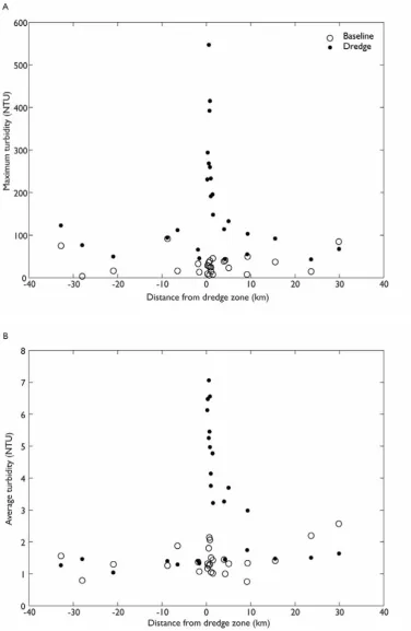
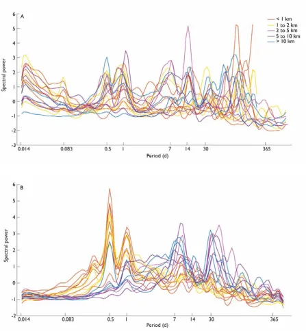
(12) List of Figures Figure 2-1 Location map showing the Barrow Island water quality sites (A - C) on the eastern side of the island and the Hay Point sites (D). 21 Figure 3-1 Measured turbidity (raw, at 10 minute intervals) time series during the entire monitoring period at Barrow Island 39 Figure 3-2 Maximum (A) and average (B) turbidity during the baseline (white dots) and dredge (black dots) periods, plotted by distance of the site from the dredge zone.. 40. Figure 3-3 Measured turbidity (raw, at 10 minute intervals) time series during the baseline period (July 2014 to August 2015) at Hay Point water quality sites 43 Figure 3-4 Hay Point project. Turbidity model and model terms at 3 representative sites. 48. Figure 3-5 A-E Barrow Island Project. Turbidity model and model terms at 6 representative sites. 55. Figure 3-6 Relationship between daily averaged RMS pressure fluctuation measurements and daily averaged turbidity at three representative Hay Point sites 57 Figure 3-7 Relationship between daily averaged RMS pressure fluctuation measurements and daily averaged turbidity at three representative Barrow Island sites 58 Figure 3-8 E Turbidity running mean percentile analysis using increasing window sizes (from 1 hour to 30 days) comparing the baseline (dotted lines) and dredge periods (solid lines) at representative Barrow Island site 64 Figure 3-9 Percentiles of turbidity running means (vertical axis) calculated using (A) 1 hour running mean window size and (B) 1 day running mean window size, plotted according to the site distance from the dredge zone during the baseline period (dots) and dredge period (circles). 66 Figure 3-10 Percentiles of turbidity running means (vertical axis) calculated using increasing window sizes (1 hour to 30 days) plotted according to the site distance from the dredge zone 67 Figure 3-11 Normalised turbidity global (time-averaged) spectral power curves across all sites for the baseline period (A) and dredge period (B). 69 Figure 3-12 Normalised wave global (time-averaged) spectral power curves across all sites for the baseline period (A) and dredge period (B).. 71. Figure 3-13 Normalised water height global (time-averaged) spectral power curves across all sites for the baseline period (A) and dredge period (B).. 72. Figure 3-14 Normalised wind global (time-averaged) spectral power curves at Barrow Island airport showing the zonal (blue) and meridional (red) directions during the baseline period (solid line) and dredge period (broken line). 73 Figure 3-15 Turbidity spectral analysis for the Barrow Island project, showing reference sites C) DUG and D) SBS. 76 Figure 4-1 Relationship between midday light attenuation coefficients (k) and turbidity (black dots) at two sites close to dredging. 94. xi.

(13) Figure 4-2 (A) Terrestrial PAR, (B) benthic PAR, (C) turbidity and (D) midday k values at MOFA (see Figure 2-1 for site locations) from September to December 2010. 96 Figure 4-3 (A) Time series of midday (10:00−14:00 h) turbidity (primary vertical axis) and light attenuation coefficients (k, secondary vertical axis) at MOFA (located ~ 500 m south of dredge zone), (B) scatter plot of turbidity and k at MOFA, (C) time series of midday (10:00−14:00 h) turbidity (primary vertical axis) and light attenuation coefficients (k, secondary vertical axis) at reference site REFS, and (D) scatter plot of turbidity and k at REFS (~25 km south of dredge zone). See Figure 2-1 for site locations. 97 Figure 4-4 Scatter plot showing the relationship between midday turbidity and light attenuation coefficients for the aggregated data during dredging, separated into near field (MOF and LNG sites < 1.4 km south of dredging, blue dots) and far field sites (all other sites, red asterix). The inset shows the zoomed region between turbidity = 0 - 4 NTU and k = 0 - 0.5 m-1 as they are difficult to compare in the main figure. Sites have been grouped to investigate whether a particle size dependency exists in the light attenuation coefficients. 98 Figure 4-5 Relationship between turbidity and the light attenuation coefficient (k) at four sites close to dredging 99 Figure 4-6 Clear water light attenuation coefficient (k0, k when turbidity = 0 NTU) plotted against the average of the dredge period midday logger depths (z) at each site. 100 Figure 4-7 Relationship between observed Iz at depth z and modelled 𝐼𝐼 using the three regression methods: linear / power comparisons are blue dots, rational function method are red dots and the Paulson Simpson double exponential method are orange dots at sites A) LNG0 and B) LNG2 during the dredge period. 103 Figure 4-8 Median midday (A) k (depth corrected) and (B) turbidity plotted according to the distance of the site from the dredge zone 104 Figure 5-1 An example of the sawtooth pattern occurring in the SSD data during significant sediment accumulation events.. 114. Figure 5-2 Average daily SSD (mg cm-2) during the baseline period (white circles) and dredge period (black circles) during the Barrow Island project plotted according to the distance of the sites from the dredge zone 115 Figure 5-3 SSD data at MOFA demonstrating the rapid removal of accumulated sediment during a two hour accumulation period 118 Figure 5-4 (A) Turbidity (black line) and deposition (orange line) at site MOFC from 19-20 August 2010, demonstrating the sawtooth pattern in the deposition data resulting from sediment accumulation and wiper action, and (B) the wavelet transform of the sawtooth pattern in deposition data, showing higher energy (yellow bands) in the 2,1 and half hour periods. 118 Figure 5-5 Daily average overburden (NTU) during the baseline period (white circles) and dredge period (black circles) during the Barrow Island project plotted according to the distance (km, see Figure 2-1) of the sites from the dredge zone 120 Figure 5-6 Overburden and daily averaged surface sediment density comparing all overburden values (black circles) and only days when overburden > 5 NTU (orange circles) at sites DUG (A) and DSGS (B). The relationship improved significantly at both sites when comparing overburden and SSD only on days when overburden > 5 123 NTU, from R2 = 0 (typical of all sites) to R2 = 0.5 at DUG and R2 = 0.7 at DSGS. Figure 5-7 Daily averaged SSD (solid line) and daily overburden (broken line) at site DUG (A, 9.3 km south of the dredge zone) and MOF1 (B, 0.8 km of dredge zone and on the perimeter of the spoil disposal ground) during the dredge period. 124 Figure 5-8 Daily overburden (A) and daily averaged sediment surface density (B) at Barrow Island sites from December 2007 to December 2011 plotted according to the distance of site from the dredge zone. Negative xii.

(14) values are north of the dredge zone (which is at origin) and positive values are south. The black dotted line separates the baseline period (December 2007 to 19 May 2010) and dredge period (19 May 2010 to December 2011). 125. xiii.

(15) List of Tables Table 2-1 Barrow Island water quality monitoring site details, including site distance from dredge zone, average logger depth, baseline monitoring length and dredge period monitoring length. 23 Table 2-2 Hay Point monitoring site details, including average logger depth and monitoring length in days.. 24. Table 3-1 Summary table showing maximum (raw and daily averaged), mean and standard deviation turbidity during the baseline (train and test periods) and dredging periods 41 Table 3-2 Summary table showing maximum (raw and daily averaged), mean and standard deviation turbidity at Hay Point sites during the baseline (train and test) period, and R2 values between the measured and modelled turbidity 44 Table 3-3 Turbidity model performance at Hay Point sites based on the R2 and skills score between modelled and measured turbidity 49 Table 3-4 Turbidity model performance at Barrow Island sites based on the R2 and skills scores between modelled and measured turbidity. 56. Table 3-5 R2 and root mean square error (RMSE) between RMS pressure fluctuations (estimates of seafloor wave motion) and turbidity measurements. 58. Table 3-6 R2 and root mean square error between RMS pressure fluctuations (quasi-estimates of wave motion at the seafloor) and turbidity measurements at Barrow Island 59 Table 4-1 Dredge period average PAR, median and maximum midday light attenuation coefficients (k) and turbidity, k in clear water (k0), and the number of days the midday averaged turbidity exceeded 50 NTU at all study sites and aggregated across all Barrow Island sites 94 Table 4-2 Relationship between midday light attenuation coefficients (k) and turbidity at Barrow Island Table 4-3 R2 and RMSE between modelled 𝐼𝐼 and measured Iz. 95 102. Table 5-1 Summary table showing mean, median and maximum SSD during the baseline and dredging periods listed according to site distances (km) from north to south of the dredge zone. 116 Table 5-2 Summary table showing mean and maximum overburden (i.e. difference between measured and modelled turbidity in NTU) during the dredge period 121. xiv.

(16) Introduction 1.1. Background. Dredging is necessary to create or expand ports and harbours and deepen shipping channels but the altered water quality conditions can be harmful to the environment, particularly sensitive benthic habitats such as coral reefs (Rogers 1990, Foster et al. 2010, Erftemeijer et al. 2012), due to increased sediment related impacts. Despite the large number of dredging projects in Australia and around the world, and concerns about associated environmental impacts, our knowledge of water quality changes during dredging and impacts to coral reefs is limited. Fortunately we now have access to the largest (spatial and temporal) water quality dataset ever collected prior to and during a large scale (~ 7 Mm3) capital dredging project at Barrow Island, Western Australia, allowing a comprehensive study into water quality changes (specifically light and deposition) during dredging, as well as development of new dredge impact analysis techniques (i.e. turbidity model) to understand the environmental impact of dredging. The main focus of this thesis will be to look at aspects of this dataset to temporally compare turbidity, light attenuation and sediment deposition prior to and during dredging, and to spatially compare these conditions to describe the distance to dredge effects at increasing distance from the dredge zone.. Due to the recent resources boom, there have been numerous large scale capital dredging projects, particularly along the Queensland coast and on Western Australia’s North West Shelf (NWS) (see McCook et al. 2015 for details). In the 2014-15 financial year, Australia’s resources minerals and petroleum sector was worth ~ $100 billion, and 86 % of Australia’s LNG exports were from the NWS. 1.

(17) (DSD 2016). The potential environmental threat of dredging has attracted contentious public interest, mostly due to our limited understanding of how dredging alters sediment related processes such as turbidity, benthic light availability and sediment deposition, and the associated environmental impacts, particularly to coral reefs. Understanding these impacts is important for managing marine ecosystems in the short- and long- term, and at regional (Fabricius et al. 2014) and local scales (Sofonia & Unsworth 2010, Fabricius et al. 2014, Chartrand et al. 2016). Knowledge gaps lead not only to public scrutiny, which can influence government decisions, but can also cause unnecessary environmental damage, operational delays and greater cost to proponents during dredging operations (due to inaccurate thresholds), as well as costly and lengthy environmental approvals process.. 1.2. Motivation. The ability to forecast the environmental impact of dredging is an important component of modelling at the EIA stage, or when dredging is underway, and is based upon the ability to understand how pressure fields (such as light reduction and elevated deposition) relate to suspended sediment concentrations (SSCs), and how these propagate in the environment. This information can be used to describe the relationship between coral health and dredging water quality pressures. Being able to predict the scale of potential impacts from dredging near coral reefs is important for dredging management, and establishing an evidence-based footprint is increasingly becoming important for public perception of the nature and scale of dredging projects (Fisher et al. 2015, Spearman 2015).. 2.

(18) Dredging proponents are required to manage projects under a spatially defined zonation scheme (EPA 2011), and limited understanding about dredging impacts can lead to inaccurate water quality thresholds, possibly resulting in unnecessary damage, operational delays and great expense to proponents. Water quality thresholds are often set conservatively (for example based on the 80th percentile of typical ambient conditions, ANZECC 1994) rather than based on evidence of environmental tolerance levels (EPA 2011). If thresholds are set too high corals may be regularly exposed to potentially stressful conditions, possibly leading to mortality. Inaccurate thresholds can also delay dredging operations and be costly for proponents; setting thresholds well below tolerance limits can prompt increased monitoring and reporting frequency (for example fortnightly, see Chevron Australia Pty Ltd 2011a), and, in the worst case scenario, can suspend dredging operations.. 1.3. Knowledge gaps. The most significant knowledge gap related to dredging impacts is the spatial extent of dredge effects. Our understanding of the distance to dredge effects is necessary for impact prediction during the EIA process, and for optimal design of dredging operation location and water quality monitoring site locations. There are a number of reasons for our limited understanding of dredging impacts. For one, there are few large (temporal and spatial) in-situ water quality datasets collected during dredging available; it is challenging placing water quality sensors close to a dredge, and data collected by industry aren’t always publicly available (Condie et al. 2006). Furthermore, water quality changes during dredging are site specific, dependent on local hydrodynamic conditions. Therefore improved understanding requires comprehensive studies on a variety of dredging projects with adequate water quality monitoring site locations. Also, (although not addressed in this 3.

(19) thesis but rather driving the need for this study) further complexities exist because coral response to water quality changes are site- and species- specific, and there are multiple cause-effect pathways which can affect corals (is reduced light or increased deposition the greatest threat?).. Complex sediment pressure and coral response relationships further challenge our understanding and management of dredging impacts. The temporary release of sediment into the water column during dredging can have a range of environmental effects on sensitive communities such as coral reefs (Marszalek 1981, Rogers 1990, Foster et al. 2010, McCook et al. 2015). The two primary causes of stress or mortality to corals during dredging are reduced light and deposition (Erftemeijer et al. 2012, Jones et al. 2016). Light (specifically photosynthetically active radiation (PAR), 400 – 700 nm) is essential for benthic primary production and light reduction, which occurs during dredging due to increased turbidity and deposition (Stoddart 1969, Kirk 1977a, Cloern 1987, Anthony & Fabricius 2000, Gattuso et al. 2006, Saulquin et al. 2013), inhibits the primary energy source for corals (Hallock & Schlager 1986, Te 1997, Anthony & Fabricius 2000, Anthony et al. 2004, Gattuso et al. 2006, Gilmour et al. 2006, Storlazzi et al. 2015). Sustained and frequent PAR reductions have well-known effects on the functioning and distribution of marine ecosystems (Kinzie 1973, Chalker 1981, Chalker et al. 1984, Graus et al. 1989, Rogers 1990, Erftemeijer et al. 2012). Deposition of the re-suspended sediment is also a well-known hazard, requiring benthic organisms to expend energy self-cleaning or become progressively smothered in sediments, which can clog their breathing and feeding apparatus. Smothering is sometimes observed in dredging projects close to reefs (Dodge & Vaisnys 1977, Bak 1978) and the reduction in gas (solute) exchange, under some circumstances, quickly lead to local tissue mortality and lesion formation (Weber et al. 2012). Deposition during calm conditions 4.

(20) can be immediate and in-situ, as the lack of resuspension hydrodynamics – wind, waves and tidal currents – are insufficient to maintain the sediment in suspension (Masselink et al. 2011). Another factor limiting our understanding of dredging impacts is the site specific nature of water quality conditions. Local bathymetric profiles and hydrodynamics determine natural water quality conditions and influence the direction and behaviour of dredge plumes which can lead to different spatial results for different dredging operations. For example, a study using satellite images of suspended sediments has suggested the dredging plume at Barrow Island travelled as far as 30 km south (Evans et al. 2012), while others have claimed, in scientific journals and the media that, using numerical simulations, very fine buoyant particles such as coal dust can travel as far as from the coast to the outer Great Barrier Reef (Burns 2014). These statements further emphasise the need for large, high spatial and temporal resolution in-situ water quality data to more accurately study the environmental impacts of dredging.. Coral response to dredging is also complex, as it is site- and species- specific. Different corals exhibit different morphological responses to sediment related pressures or different light environments (due to different depths), and these responses can also be developed differently according to the ambient water quality conditions (Falkowski et al. 1984). Cooper et al. (2008) suggest that chronic (long term) turbidity levels > 3 and > 5 NTU result in sub-lethal and severe stress to corals, and Flores et al (2012) found similar results from lab experiments with total mortality occurring after 12 weeks of exposure to 30 & 100 mg L-1 (which approximately converts to 30 – 200 NTU for the Barrow. 5.

(21) Island data based on the provided conversion values) depending on the species. In contrast, Browne reported little to no mortality to corals exposed to pulsed moderate turbidity (~ 50 mg L-1) in the lab for up to 1 month. Furthermore, the response of corals to changes in water quality can be location specific; the same species can become adapted to naturally clearer water or more turbid environments (Newell et al. 1998).. Although corals can survive from naturally elevated sediment-related disturbances caused by storms and cyclones (Shinn 1976, Woodley et al. 1981, Riddle 1988, Carter et al. 2009, Connell 1997), dredging can increase SSC to unnatural levels for prolonged periods, restricting recovery time between events (Gilmour et al. 2006, Jones, Fisher, et al. 2015). Natural resuspension can increase SSC to levels as high as occurs during dredging (Gagan et al. 1990, Green 1995, Orpin et al. 1999, McKinnon et al. 2003, Gilmour et al. 2006, Guillén et al. 2006, Carter et al. 2009), and, although there have been reports of coral reef destruction (depending on the severity of the storm and habitat depth) (Harmelin-Vivien & Laboute 1986, Done 1992, Dollar & Tribble 1993, Tomascik et al. 1994), such events are usually short lived (Dollar & Tribble 1993, Onuf 1994, Anthony et al. 2004) and the ecosystems are typically adapted to these conditions and can even benefit from the removal of sediment during storms. Resuspension due to dredging, however, may occur for longer, more frequently and during calm conditions. Previous studies show dredge related water quality changes were confined to an area close to dredge zones; in Cleveland Bay, deposition rates were 10 x higher at sites within 500 m of dredging than at sites 1.5 km away (Kettle et al. 2001) and, in Mermaid Sound (Dampier Archipelago on Western Australia’s NWS), Stoddart and Anstee (2004) reported. 6.

(22) average turbidity levels decreased from 3.75 NTU at sites within 1 km of dredging to 1.24 NTU at far field sites. The consequences of our lack of understanding of dredging impacts are significant. The health of the Great Barrier Reef (GBR) and our oceans are important to the Australian public, but we are also reliant on the resources sector and large minerals and mining exports, which requires ship movements and suitable ports for export. Recently there has been increased public scrutiny about the impacts of dredging on coral reefs due to the expansion of a number of Queensland ports (e.g. Abbot Point and Gladstone Harbour) and associated dredging operations. Multiple pressures from the public and environmental lobby groups about the impacts of dredging and dredge spoil disposal have resulted in government intervention, particularly related to the Abbot Point and Gladstone Harbour dredging programs despite inconclusive evidence from multiple scientific organisations (including research by the Queensland Department of Environment and Heritage Protection, Queensland Department of Agriculture, Fisheries and Forestry, CSIRO, and the University of Tasmania) that dredging or dredge spoil disposal directly impacts local ecosystems (Environment and Communications References Committee 2014). This public scrutiny and lack of evidence into the impacts of dredging highlights the need for large water quality studies during dredging operations and comparisons to local ambient water quality conditions.. 1.4. Aims and objectives. Using the largest water quality dataset ever collected prior to and during a large scale capital dredging project, this thesis aims to describe the distance to dredge effects on sediment related pressures. Although this data was not studied while the dredging operation was underway due to. 7.

(23) limited time and resources, many aspects of the data are described here to better understand the temporal and especially the spatial impacts of dredging on water quality conditions. The aims of this thesis are briefly outlined here and each aim is expanded below: 1. To broadly describe (spatially and temporally) turbidity changes during dredging at Barrow Island to better understand dredging related sediment pressures. Temporal analysis involves comparing baseline (pre-dredge) turbidity to dredge turbidity, and spatial analysis compares turbidity conditions at increasing distances from the dredge zone. 2. More specific temporal investigation of turbidity used a running mean analysis with increasing running mean window sizes to investigate turbidity extremes over increasing time frames. 3. Spectral methods were also used to study the temporal behaviour of turbidity. A wavelet analysis technique identified natural periodic resuspension drivers (i.e. semi-diurnal tides, daily sea breeze etc.), and comparison between the baseline and dredge periods investigated the impacts of dredging on these. 4. A simple empirical turbidity model was developed to estimate natural turbidity conditions from seafloor pressure measurements (estimates of the influence of waves and tides on the seafloor). The model is designed to be a simple alternative to the complex three dimensional hydrodynamic models typically used for suspended sediment estimates which require vast measurements across a large spatial area (which are often not available), and can provide an simple estimate of dredge induced turbidity as a first response threshold exceedance tool and can contribute to research into dredge impacts on coral reefs. 8.

(24) 5. The impacts of dredging on underwater light conditions was also temporally and spatially analysed. Light attenuation coefficients were investigated in lieu of PAR measurements to study the distance to dredge impacts on submarine light levels. 6. Sediment deposition conditions prior to and during dredging, and at increasing distance from the dredge zone, were also studied using in-situ sediment surface density measurements and overburden calculations from the turbidity model. The ability of the overburden to be used during future dredging operations to monitor dredge related deposition was also investigated by comparing overburden to SSD measurements.. To better understand the impacts of dredging, this thesis explores distance to dredge effects on sediment-related processes during dredging, and investigates the use of a simple, statistical turbidity model to estimate natural turbidity during dredging so that turbidity levels caused solely by dredging can be estimated and used to further study the impacts of dredge sediment pressures on coral health. The spatial and temporal impacts on turbidity, light attenuation and sediment deposition conditions are investigated by comparing baseline (pre-dredge) conditions to dredge conditions, and spatially the distance to dredge effects are explored by comparing conditions at increasing distances from the main dredge zone. The model was developed and optimised in two different hydrodynamic settings (Barrow Island and Hay Point) to assess performance in different environments. Use of the model to estimate dredge related deposition was also investigated.. 9.

(25) Temporal and spatial analysis of turbidity conditions were analysed at Barrow Island prior to and during dredging to characterise the ambient water quality conditions and better understand dredging impacts on these. Baseline turbidity levels were compared to dredging conditions, and, for both monitoring periods, turbidity levels compared at increasing distance from the dredge zone to investigate the distance to dredge effects. Common statistical methods were used (e.g. mean, median and standard deviation) as well as an running mean analysis and spectral analysis.. Running mean temporal analysis (with increasing running mean window sizes) was adopted to investigate turbidity characteristics and extremes over a range of time frames, due to the complex response of corals to changes in their environment (e.g. corals may be able to withstand acute changes but may suffer under prolonged or frequent baseline exceedance). Spectral analysis was also performed on turbidity, wind, wave and water height (tidal) data to better understand natural resuspension drivers and the impact of dredging on these. Spectral analysis can reveal the natural turbidity conditions in a region: i.e. are the daily resuspension events due to sea breezes or diurnal tides, and do the semi-diurnal and spring / neap tides influence resuspension? Comparing the baseline spectral results to those during dredging can also provide insight into the impact dredging has on natural resuspension events.. A simple empirical turbidity model was developed to predict natural turbidity events from seafloor pressure measurements induced by waves and tides (Larcombe et al. 1995, Jing & Ridd 1996, Ogston et al. 2004, Presto et al. 2006, Condie & Andrewartha 2008, Fettweis et al. 2010, Verspecht &. 10.

(26) Pattiaratchi 2010, Erftemeijer et al. 2012). Seafloor pressure measurements provided model predictor variables – estimates of the influence of waves, water height, tidal range and tidal currents on sediment resuspension. Sediment suspension occurs due to high frequency wave orbital velocities and wind and tidal current velocities occurring in the bottom boundary layer immediately above the seafloor, which induce a shear stress on seafloor sediment that results in sediment suspension once a critical threshold is exceeded (Grant & Madsen 1986). Typically, complex three dimensional hydrodynamic and wave models are used to estimate sediment suspension and sediment transport, however these models require vast inputs which are often unavailable (either not collected or privately owned) and expensive to collect, particularly during dredging operations which are already very expensive operations. Therefore, a simple empirical model using only seafloor pressure measurements (estimates of the influence of waves and tides on the seafloor) was tested as an inexpensive alternative. Although wave orbital velocities were unable to be measured using pressure measurements due to the low sampling frequency, and therefore high resolution estimates of natural turbidity conditions are likely not possible, lower resolution (daily) estimates of natural turbidity conditions were attempted.. Model predictors were calibrated to baseline turbidity measurements and model performance was validated using out-of-sample baseline data i.e. a future section of the baseline time-series which was not used to train the model input variables to the measured turbidity. The model was applied in two different hydrodynamic settings – the clear waters of Barrow Island and the highly turbid environment of Hay Point, North Queensland. A feature of the model is its simplicity; it only requires collection of at least two variables – seafloor turbidity and water pressure – and the model provides 11.

(27) a simple method to decouple natural and dredge related turbidity events. As turbidity measured during dredging is a combination of both natural and dredged turbidity, coupling makes it difficult to assess if threshold exceedance or environmental damage is caused by dredging or due to natural disturbance (for example Onuf 1994). The difference between the measured (dredged + natural) and modelled (natural) turbidity provides an estimate of turbidity caused solely by dredging – called overburden from herein – offering improved insights into dredging impacts.. Further understanding of dredging impacts were achieved by studying changes to submarine light conditions prior to and during dredging, and analysing the relationship between light and turbidity conditions. Light attenuation was used to describe the light environment in this thesis, assuming that light decay in coastal waters can be approximated (at least to a first order) by the attenuation coefficients calculated using the Beer Lambert Law (Gallegos 2001). Attenuation coefficients were used in lieu of PAR or daily light integrals (DLI), due to the non-uniform water quality sensor depths (ranging from 3.5 – 14 m) and due to their inherent exclusion of atmospherically derived interference in the submarine light levels (i.e. because the attenuation coefficient is only concerned with irradiance decay from the surface to depth z it is unaffected by attenuation due to cloud cover). In contrast, PARs or DLIs provide simply a measure of the light at depth z, and, although sufficient to demonstrate benthic light conditions, do not specify the source of the light decay therefore possibly obscure dredging impact analysis.. 12.

(28) Light is attenuated in the water column through scattering and absorption by water (Kirk 1977b) and water contents. In coastal waters, absorption is mostly by water molecules and scattering by suspended sediments (Kirk 1977b, Cloern 1987, Mobley 2001, Margvelashvili et al. 2006, Lawson et al. 2007, Saulquin et al. 2013). Coastal water attenuation coefficients typically range from 0.1 – 6 m-1 (Kirk 1977b, Baker & Lavelle 1984, Anthony et al. 2004, Piniak & Storlazzi 2008, Devlin et al. 2008, Saulquin et al. 2013), while on the NWS (Cape Lambert) coefficients were between 0.1 and 3.5 m-1 (In-Situ Marine Optics 2011) and in Queensland between 0.3 and 1 m-1 (Anthony et al. 2004). Inland waters have much higher attenuation coefficients – up to 15 m-1 (Devlin et al. 2008), due to the high absorption and scattering properties of yellow substances, or gilvin (Kirk 1977b, Bowers et al. 2000). In contrast, in the clear, deep open ocean waters, phytoplankton are relatively important in absorbing and scattering light (Smith & Baker 1978, Cloern 1987, Saulquin et al. 2013). Previous studies in Cleveland Bay have found light attenuation to be strongly related to suspended sediments, with 74 – 79 % variance in light attributed to SSCs (Anthony et al. 2004). The scattering of light by suspended particles not only reduces benthic light availability by diffracting light away from the benthos, but the consequent extended path length increases the probability that light will be absorbed by water molecules (Kirk 1985).. Dredging can dramatically decrease submarine light levels. Chartrand et al. (2008) reported light levels reduced to near darkness for most of the dredging program at Hay Point, measured using two light sensors approximately 16 km apart on the edges (southern and western) of the dredge plume impact area (although it is unclear the depth of the light sensors). Bak (1978) found that surface. 13.

(29) irradiance had reduced from 30 % to 1 % at a depth of 12 – 13 m, and Onuf (1994) estimated attenuation coefficients increased from 1 – 1.35 m-1 before dredging to 1.5 – 2.1 m-1 after.. Attenuation of light due to absorption by water molecules is wavelength dependent, and therefore depth dependent (Sverdrup 1953, Kinzie 1973, Kirk 1977b, Saulquin et al. 2013, Storlazzi et al. 2015). Longer wavelengths (the red part of the spectrum) are absorbed more strongly than the shorter waves (Kirk 1977b, Saulquin et al. 2013, Storlazzi et al. 2015), and are therefore rapidly absorbed in the surface layers. This increases the absorption attenuation rate and depletes red light in the upper layers, leaving the less easily absorbed shorter wavelength light (blue-green) in the underlying layers. Consequently, the attenuation rate is higher in the surface layers, introducing a depth dependence to the attenuation coefficient (Kinzie 1973, figure 4 in Jewson et al. 1984, Schanz 1985). Paulson and Simpson (1977) provide an alternative double exponential function derived from the Beer Lambert Law to allow for this depth dependence. The Beer Lambert Law was converted into the double exponential function which includes a term for higher attenuation near the surface (upper 5 m according to the authors) and a separate term for the lower attenuation rate of the remaining blue-green light at depths > 10 m: (1). 𝐼𝐼 ⁄𝐼𝐼0 = 𝑅𝑅𝑒𝑒 𝑧𝑧⁄𝜁𝜁1 + (1 − 𝑅𝑅)𝑒𝑒 𝑧𝑧⁄𝜁𝜁2. The first term on the right hand side (RHS) represents the higher attenuation in the upper layers and the second term represents the lower attenuation rate in the deeper layers. Values for R and. ζ2 were obtained by a least squares fit of 𝐼𝐼 ⁄𝐼𝐼0 = (1 − 𝑅𝑅)𝑒𝑒 𝑧𝑧⁄𝜁𝜁2 to observed light levels at depths > 10 m, then a second least squares fit of equation 1 was applied to observed light levels < 6 m to get. 14.

(30) a value for ζ1. In addition to using the original Beer Lambert Law in this study to investigate light attenuation during dredging, the alternative Paulson and Simpson method was also investigated (see Chapter 4).. Previous studies have suggested that sediment particle size distribution can also influence light scattering (Jonasz & Fournier 2007, Kirk 2010). Storlazzi (2015) and Te (1997) both found higher attenuation coefficients for smaller grain size (e.g. mud compared to sand for Storlazzi, and terrigenous vs carbonate silt for Te). As dredging can alter sediment particle size distribution (PSD) by increasing the proportion of fine particles close to the dredge zone (Jones et al. 2016), differences in attenuation coefficient ranges were compared at sites close to dredging to further reference sites.. Excess suspended sediment during dredging can also lead to increased deposition as the sediment falls out of suspension, depositing on the benthos and corals. Sediment accumulation on corals can be as harmful, if not more, to corals as other suspended sediment related impacts such as reduced light (Jones et al. 2016). Deposition during dredging is more likely to be immediate and less dispersed than during natural deposition events (i.e. storms and cyclones) as the lack of resuspension hydrodynamics – wind, waves and tidal currents – are insufficient to maintain the sediment in suspension (Masselink et al. 2011). Furthermore, in the absence of high waves or strong currents the deposited material will likely remain on sensitive benthic communities.. 15.

(31) In this study, several dredge related deposition analysis methods were investigated, including deposition sensor data and use of the turbidity model overburden. Model overburden (calculated by subtracting daily modelled from measured turbidity) estimates excess turbidity caused by dredging, and could also predict dredge related deposition. This is based on the assumption that excess turbidity above natural levels – particularly in calm conditions – is likely to result in immediate in-situ deposition due to the absence of resuspension hydrodynamics – high wind, wave and tidal activity (Green 1995, Larcombe & Woolfe 1999, Pearce et al. 2003, Storlazzi et al. 2004, Orpin et al. 2004, Condie & Andrewartha 2008, Fettweis et al. 2010). These turbulent conditions are necessary to maintain sediment in suspension and to disperse sediment from the source. Without them, excess turbidity is likely to immediately deposit and remain at the deposition site until sufficient wave activity can remove it (Spearman 2015, Jones et al. 2016).. The work in this thesis is also presented in 2 reports (1 submitted, 1 published) for the Western Australian Marine Science Institution’s Dredging Science Node, 1 report for the North Queensland Bulk Ports Corporation (NQBP) (published), and 4 journal articles (2 published, 2 in preparation). Further details on which reports and papers the contents of this thesis appear in, as well as my contribution to each, are provided here: WAMSI DSN reports:. •. Fisher R, Stark C, Ridd P, Jones R (2014). Project 4.2. Effects of dredging and dredging related activities on water quality: Phase 1 - spatial and temporal patterns (published). o The running mean varying temporal analysis, spectral analysis and light attenuation analysis in this report were produced by myself and are included in this thesis in Chapter 3 (running mean and spectral analysis) and Chapter 4 (light attenuation. 16.

(32) analysis). The running mean analysis is also included in the journal article Jones et al. (2015) listed below. •. Stark C, Whinney J, Ridd P, Jones R (submitted 2016). Project 4.4. Estimating sediment deposition fields around dredging projects. o Analysis and results of the turbidity model at Barrow Island presented in the report appears in Chapter 3 of this thesis, and model overburden and in-situ deposition analysis and results are used to describe a dredge deposition zone in Chapter 5. This report will be submitted for publication as a journal article, listed below.. NQBP report:. •. Waltham, N., McKenna, S., York, P., Devlin, M., Campbell, S., Rasheed, M., Da Silva, E., Petus, C., Ridd, P., 2015, ‘Port of Mackay and Hay Point Ambient Marine Water Quality Monitoring Program (July 2014 to July 2015)’, Centre for Tropical Water and Aquatic Ecosystem Research (TropWATER) Publication 15/16, James Cook University, Townsville, 96 pp. •. Waltham, N., McKenna, S., York, P., Devlin, M., Campbell, S., Stark, C., Rasheed, M., Da Silva, E., Petus, C., Ridd, P., (submitted), ‘Port of Mackay and Hay Point Ambient Marine Water Quality Monitoring Program (July 2015 to July 2016)’, Centre for Tropical Water and Aquatic Ecosystem Research (TropWATER) o The turbidity model analysis and results at Hay Point from Chapter 3 of this thesis are presented in these reports. Journal publications:. •. Stark C, Ridd P, Fisher R, Jones R (in preparation). Dredging spatial impacts on light attenuation o Chapter 4 of this thesis will be submitted as a journal article and is in preparation.. •. Stark C, Whinney J, Ridd P, Jones R (in preparation). Estimating sediment deposition fields around dredging projects. o Chapter 5 of this thesis will be submitted as a journal article and is in preparation.. •. Fisher R, Stark C, Ridd P, Jones R (2015). Spatial patterns in water quality changes during dredging in tropical environments. PLoS One. 17.

(33) o My contribution to this paper included construction and analysis of raw turbidity across all Barrow Island sites for the baseline and dredge periods (Figure 6) which also appears in this thesis as Figure 3-1.. •. Jones RJ, Fisher R, Stark C, Ridd P V (2015). Temporal Patterns in Seawater Quality from Dredging in Tropical Environments. PLoS One. o My contribution to this paper included the running mean varying temporal analysis which appears in this thesis in Chapter 3 section 3.3.4.. 1.5. Document Organisation. Chapter 1 summaries the rationale and context for this work and discusses the research objectives and scope of thesis.. Chapter 2 presents information about the study sites and data collection instruments (data analysis methods for chapters 3 – 5 are included in each chapter).. Chapter 3 presents spatial and temporal analysis of turbidity conditions prior to (baseline period) and during dredging at Barrow Island and briefly describes turbidity conditions at Hay Point, North Queensland (where water quality sites were used to further analyse model performance). Temporal analyses includes running mean analysis using increasing running mean window sizes to investigate extreme conditions and the temporal range of dredging effects, and spectral analysis was applied to turbidity, wind, wave and water height data to investigate periodic events and identify resuspension driving mechanisms, and whether dredging impacted natural resuspension events.. 18.

(34) The turbidity model applied to the Barrow Island and Hay Point water quality sites is also presented in this chapter.. Chapter 4 presents analysis of underwater light conditions during dredging. This study is unique in that the depth dependence of the light attenuation coefficient was removed to improve the spatial accuracy of dredging impacts on submarine light levels. To investigate the relationship between dredging impacts and light, light attenuation coefficients were compared to turbidity levels.. Chapter 5 investigates the effects of dredging on deposition accumulation. In-situ sediment accumulation data as well as overburden (estimated excess turbidity from dredging) calculated from the turbidity model were analysed to identify a dredge deposition zone and to investigate the use of a simple turbidity model for monitoring dredge threshold exceedance.. Chapter 6 presents the conclusion of the research and recommendations for possible future work. Key findings are presented in this chapter.. 19.

(35) Sites and data 2.1. Study sites. The primary data used during this thesis is globally the largest water quality dataset every collected during a dredging operation. Dredging for construction of the materials offloading facility (MOF) and LNG jetty of the new Gorgon LNG plant at Barrow Island, Western Australia – the “largest single resource. development. in. Australia’s. history”. (see. https://www.chevronaustralia.com/our-. businesses/gorgon) – lasted for 18 months from 19 May 2010 – 31 November 2011. Prior to and. during dredging, water quality and water pressure measurements were collected at up to 29 sites along a 60 km north / south transect for up to 4 years. A high density of water quality sites were positioned close to the dredge area (10 of the 29 sites), and two water quality sites were placed on the perimeter of the dredge spoil disposal ground which is located ~ 5 km from the main dredge zone (see Figure 2-1). Baseline monitoring began as early as December 2007 at some sites.. Barrow Island is located approximately 120 km from the Pilbara in Western Australia. On the eastern side of the island (the location of the dredging project and water quality monitoring sites) it is considered a clear water environment (Hubbert et al. 2005) with naturally low ambient SSC levels typically < 5 mg L-1 (Jones, Ricardo, et al. 2015). Hydrodynamics in the Barrow Island region are generally driven by strong currents and a moderate tidal range, and are also influenced by wind and wave action (DEC 2007). The shallow bathymetry (≤ 20 m), coral reefs and shoals between the island and mainland produce complex flows (Hubbert et al. 2005). Tidal currents, moving from offshore in a cross-shelf direction (which are oriented east-west around Barrow Island, Condie & Andrewartha 2008), diffract around the north and south of the island and converge on the eastern side between 20.

(36) the Lowendal Shelf and Dugong Reef (abbreviated to DUG in Figure 2-1) (Hubbert et al. 2005). Some of the water quality monitoring sites are protected on the lee of the island from offshore waves (Pearce et al. 2003, DEC 2007), adding to the complex flows and clear waters. There are fringing sub-tidal coral reefs around Barrow Island – estimated by the former Department of Environment and Conservation (now Department of Environment and Regulation) at ~ 150 hard coral species within the Barrow Island and Montebello nature reserves in 2007 (DEC 2007).. Figure 2-1 Location map showing the Barrow Island water quality sites (A - C) on the eastern side of the island and the Hay Point sites (D). Map A shows all water quality sites along the 60 km north / south transect. There are two main dredging areas with MOF and LNG water quality sites (map C), and a dredge spoil disposal ground approximately 5 km from the main dredging zone with sites LONE and DSGS on the perimeter. Map C also shows the depth contours of the higher resolution sites close to the materials offloading facility (MOF) and LNG access jetty. Map B shows the location of Barrow Island relative to the north western Australian Coast. Map D shows the Hay Point water quality sites (see Waltham et al. (2015) for further Hay Point site location details).. A second dataset was also used during this study to test and validate the turbidity model. Baseline water quality monitoring was conducted at Hay Point, Queensland, to ensure minimal 21.

(37) environmental impact during future routine maintenance dredging. Data was collected at 6 sites for 2 years from 05 July 2014 – 25 July 2015 and provided by the North Queensland Bulk Ports Corporation (Waltham et al. 2015). Note that the monitoring period for the Waltham et al. (2015) report only included the first year of data.. The Port of Hay Point, located ~ 40 km south of Mackay, is one of the largest global coal export facilities, transporting 115 million tonnes in 2014 / 2015 (NQBP 2015). Hay Point and Mackay are much more energetic, turbid environments than Barrow Island (Waltham et al. 2015), with significantly higher wave heights than other Queensland regions (Orpin et al. 1999, Chartrand et al. 2008, Macdonald et al. 2013, Waltham et al. 2015) where resuspension can occur at sites > 20 m depth (Orpin et al. 1999). Wind was predominantly from the S-SE during the study period (Waltham et al. 2015). Hay Point has fringing coral reefs, sparse seagrass and algal communities (Macdonald et al. 2013).. Water quality site details for both studies are provided in Table 2-1 (Barrow Island) and Table 2-2 (Hay Point), including average logger depth and deployment monitoring lengths in days. Barrow Island details also include distance of sites from the main dredge zone (see Table 2-1 for location of dredge zone) and the dredge period monitoring length.. 22.

(38) Table 2-1 Barrow Island water quality monitoring site details, including site distance from dredge zone, average logger depth, baseline monitoring length and dredge period monitoring length.. Monitoring length (d) Dredge. Distance from dredge zone (km). Average logger depth (m). 32.8 28 21 8.8 6.5 1.9 1.6 1.6. 7 7.5 7.8 4 2.1 3 7 4.5. 597 88 130 675 185 611 214 2. 484 356 346 364 377 447 436 459. 0.2 0.3 0.5 0.7 0.6 0.7 0.8 1 1 1.4 1.5 4 5 9.2 15 24 30. 8.6 11.8 8.9 10.2 4.9 6.9 6.3 7.5 6.8 10.7 4.8 6.3 4.6 5.9 3.8 5 4.8. 427 112 583 91 138 118 635 117 575 244 559 574 253 766 543 137 561. 468 475 471 486 459 449 489 506 501 475 457 483 436 457 404 364 440. Dredge spoil disposal ground* LONE 4.2 DSGS 9.2. 9.9 13.2. 592 120. 473 373. Sites Northern sites AHC REFN ELS ANT DIW LOW LOW1 LOW3 Southern sites LNG0 LNGA LNG1 LNGB MOFA MOFC MOF1 MOFB LNG2 LNGC MOF3 LNG3 TR DUG BAT REFS SBS. * Distance to spoil ground = 0.1 km. 23. Baseline.

(39) Table 2-2 Hay Point monitoring site details, including average logger depth and monitoring length in days.. Sites. Average logger depth (m). Monitoring length (d). 10.1 6.8 8.6 11.9 9.3 6.4. 296 384 378 386 387 386. Hay Reef Freshwater Point Keswick Island Round Top Island Slade Islet Victor Island. *No dredging occurred during the Hay Point monitoring, the spoil ground site is purely for baseline analysis. 2.2. Data. Both Barrow Island and Hay Point monitoring used the James Cook University Marine Geophysics Lab water quality monitoring sensors. These sensors have also been used for water quality studies for the Port of Townsville (GHD 2009a) and Western Basin dredging in Gladstone Port (GHD 2009b). Turbidity, PAR, sediment deposition and water pressure were measured every 10 minutes with sensors mounted to a logger placed on the seafloor. Sensors sit approximately 40 cm above the bed, and all sensors have mechanical antifoul wipers attached, which activate every 2 hours to prevent biofouling, allowing much longer deployments without the need for regular cleaning (Ridd & Larcombe 1994, Chevron Australia Pty Ltd 2011b, Waltham et al. 2015).. 2.2.1. Turbidity and deposition measurement and calibration. Turbidity and sediment deposition are both measured using optical backscatter sensors, which transmit infra-red light and detects the intensity of light scattered at 180° to the transmission sensor. Typically, OBS measure nephelometric turbidity units (NTU) with detectors oriented at 90° from the transmitter, however the JCU detectors are oriented at 180° to enable cleaning of the sensor plate (Waltham et al. 2015) the wiper.. 24.

(40) The turbidity sensor (in units of NTU) faces horizontally and therefore measure light scattering due to water column turbidity while the deposition sensor (also in units of NTU) faces vertically and measure the amount of sediment depositing on the sensor (Ridd et al. 2001, Thomas et al. 2003). From these two measurements, surface sediment density (SSD, in mg cm-2) are calculated and calibrated. First the water column turbidity reading (from the horizontal facing OBS) is subtracted from the deposition sensor reading (vertical facing OBS) to calculate sediment accumulation (i.e. without the water column turbidity). Then these raw OBS calculations are converted to SSD by multiplying by a site-specific calibration factor to convert to SSD in mg cm-2. The calibration factor is derived from the relationship between NTU and SSD, which is determined by calibrating the turbidity measurements with SSD measurements. In a vertical fall tower approximately 3 m high, an OBS is placed alongside a standard mass balance at the bottom of the tower. The tower is filled with water, and sediment from the site is released into the tower. Simultaneous measurements from the OBS and mass balance are recorded, and the slope of the resulting sediment density / turbidity curve provides the calibration factor to convert deposition OBS readings in NTU to SSD readings in mg cm-2.. 2.2.2. Photosynthetically active radiation and water pressure. PAR were measured using an upwards facing light sensor measuring in units of µE m-2 s-1, and water pressure fluctuations were measured using an absolute pressure sensor, which were converted to water depth in metres. The ten minute water depth measurements consisted of 1 second readings for 10 seconds, which were also used to calculate wave height. The root mean square pressure. 25.

(41) fluctuation (RMS), which measures the variance in water height from the mean, provides an estimate of wave affects at the seafloor:. 𝑛𝑛. 1 𝑋𝑋𝑟𝑟𝑟𝑟𝑟𝑟 (𝑡𝑡) = � �(𝑥𝑥𝑖𝑖 − 𝑥𝑥̅ )2 𝑛𝑛. (2). 𝑖𝑖=1. where Xrms(t) is the RMS pressure fluctuation at time t, n is the number of samples (ten), xi is the ith pressure sample, and 𝑥𝑥̅ is the mean of the ten pressure samples.. Terrestrial PAR data, used as the surface light to calculate the light attenuation coefficients, was collected on Barrow Island (339974E, 7701581N) every 15 minutes from April 2010 to February 2012 during the dredging period only (Chevron Australia Pty Ltd 2011c).. Wind data, used as a model input variable and for spectral analysis at Barrow Island, was recorded every 3 hours at Barrow Island airport and provided by the Bureau of Meteorology (Station ID: 005094, Bureau of Meteorology 2014).. 26.

(42) Temporal and spatial impacts of dredging on turbidity 3.1. Synopsis. To better understand environmental dredging impacts and to improve monitoring accuracy of future dredging operations, this chapter sought to describe the turbidity environment during a large scale capital dredging operation, to determine the spatial extent of dredging effects, and to compare dredging conditions to baseline (ambient) conditions.. A variety of temporal analyses were used, including running means using increasing running mean window sizes, to analyse extreme turbidity events and temporal changes in turbidity levels over a range of timeframes, as well as spectral analysis (using a wavelet method) – to understand the behaviour of natural turbidity drivers (daily seabreeze, semi-diurnal and spring / neap tides), and to determine whether dredging had an impact on these. A turbidity model was developed to estimate natural turbidity conditions.. A simple, statistical turbidity model was also developed to predict natural turbidity events, and its performance investigated in two different hydrodynamic settings – the clear waters of Barrow Island and the more turbid environment of Hay Point, North Queensland. The turbidity model provides a simple method to monitor dredge induced turbidity threshold exceedance during. 27.

(43) dredging operations, by decoupling the natural and dredge related turbidity levels. The use of the model to also monitor dredge related deposition is investigated in 5.3.2 Overburden.. 3.2. Methods. 3.2.1. Running mean temporal analysis. The temporal behaviour of turbidity events over increasing intervals were analysed to characterise the duration of heightened turbidity levels during dredging. The running means of the raw turbidity data were calculated at each site using increasing running mean window sizes (from 1 hour to 30 days): 𝑁𝑁𝑇𝑇. 1 𝑥𝑥̅ 𝑇𝑇 (𝑡𝑡) = � 𝑥𝑥𝑖𝑖 (𝑡𝑡) 𝑁𝑁𝑇𝑇. (3). 𝑖𝑖=1. where 𝑥𝑥̅ 𝑇𝑇 (𝑡𝑡) is the mean value calculated over the previous T hours of the data from time t-T to time t hours, and xi(t) are the NT data points up to and including time t. To avoid false averages and. percentile estimates, no 𝑥𝑥̅ 𝑇𝑇 value was recorded if more than 20% of the data points for any particular running mean period were missing.. The different running mean window sizes are used to describe turbidity conditions over a range of temporal scales. Running mean window sizes ranged from 1 hour to 30 days, and windows were increased using either a 1 hour increment for window sizes from 1 – 24 hours or a 1 day increment for larger window sizes from 1 – 30 days. For example, the first running mean applied to the turbidity data used a 1 hour window size (i.e. 6 of the 10 minute interval data points were used for each. 28.

(44) running average), then the window size was increased to 2 hours (i.e. 12 data points were used for each running average), up to 24 hours. The next running mean window size incremented to 2 days, then daily up to 30 days. Each running mean value was recorded as the mid-point of the window; for example between 10 am and 11 am, the one hour mean was recorded as 10:30 am. These running means were calculated separately for the baseline and dredge periods for comparison.. The percentiles of each running mean window were then calculated over all running mean temporal scales to characterise the duration of turbidity events, from 1 hour to 30 days. Percentile values chosen were maximum, 99th, 95th and 80th and were calculated for each turbidity average (i.e. the 4 percentiles were calculated for the 1 hour averages, then for the 2 hour averages etc. up to the 30 day averages).. 3.2.2. Spectral analysis. Temporal periodicities of turbidity, wind, wave and water height data were analysed at each site and compared between study sites to investigate the dominant periodic turbidity cycles, their driving mechanisms (tides, waves) and determine any differences between the baseline and dredge periods.. The wavelet transform method was developed by Torrence and Compo (1995), and bias correction developed by Liu et al. (2007) (detailed below). The wavelet transform detects periodic events. 29.

No results found