Spatial Patterns in Water Quality Changes
during Dredging in Tropical Environments
Rebecca Fisher1,2,3*, Clair Stark2,4, Peter Ridd2,4, Ross Jones1,2,3
1Australian Institute of Marine Science, Perth, Western Australia, Australia,2Western Australian Marine Science Institution, Perth, Western Australia, Australia,3Oceans Institute, University of Western Australia, Perth, Western Australia, Australia,4School of Engineering and Physical Sciences, James Cook University, Townsville, Queensland, Australia
Abstract
Dredging poses a potential risk to tropical ecosystems, especially in turbidity-sensitive envi-ronments such as coral reefs, filter feeding communities and seagrasses. There is little detailed observational time-series data on the spatial effects of dredging on turbidity and light and defining likely footprints is a fundamental task for impact prediction, the EIA pro-cess, and for designing monitoring projects when dredging is underway. It is also important for public perception of risks associated with dredging. Using an extensive collection ofin situwater quality data (73 sites) from three recent large scale capital dredging programs in Australia, and which included extensive pre-dredging baseline data, we describe relation-ships with distance from dredging for a range of water quality metrics. Using a criterion to define a zone of potential impact of where the water quality value exceeds the 80th percen-tile of the baseline value for turbidity-based metrics or the 20thpercentile for the light based metrics, effects were observed predominantly up to three km from dredging, but in one instance up to nearly 20 km. This upper (~20 km) limit was unusual and caused by a local oceanographic feature of consistent unidirectional flow during the project. Water quality log-gers were located along the principal axis of this flow (from 200 m to 30 km) and provided the opportunity to develop a matrix of exposure based on running means calculated across multiple time periods (from hours to one month) and distance from the dredging, and sum-marized across a broad range of percentile values. This information can be used to more formally develop water quality thresholds for benthic organisms, such as corals, filter-feed-ers (e.g. sponges) and seagrasses in future laboratory- and field-based studies using environmentally realistic and relevant exposure scenarios, that may be used to further refine distance based analyses of impact, potentially further reducing the size of the dredging footprint.
a11111
OPEN ACCESS
Citation:Fisher R, Stark C, Ridd P, Jones R (2015) Spatial Patterns in Water Quality Changes during Dredging in Tropical Environments. PLoS ONE 10 (12): e0143309. doi:10.1371/journal.pone.0143309
Editor:Silvia Mazzuca, Università della Calabria, ITALY
Received:June 30, 2015
Accepted:November 3, 2015
Published:December 2, 2015
Copyright:© 2015 Fisher et al. This is an open access article distributed under the terms of the
Creative Commons Attribution License, which permits unrestricted use, distribution, and reproduction in any medium, provided the original author and source are credited.
Data Availability Statement:There are very detailed tables and Figures in the manuscript and in the supporting information files containing all the relevant data. A metadata record is available from the Australian Institute of Marine Science at:http://data. aims.gov.au/metadataviewer/faces/view.xhtml?uuid = a884e0ab-1a82-4871-8f39-18c20ab4c9fb.
Introduction
Dredging and dredge material (spoil) disposal releases sediments into the water column, creat-ing turbid plumes that can drift onto nearby marine habitats [1]. The elevated suspended sedi-ment concentrations and the eventual settlesedi-ment of the sedisedi-ments can have a range of negative effects on benthic filter and suspension feeding organisms [1–7]. By altering the characteristics of underwater light, the increased turbidity can also have marked effects on primary producers. This is of particular significance for habitat-forming groups such as corals and seagrasses, as their loss would also result in loss of the habitat-associated biodiversity [8,9]. There are many examples of dredging programs that have had widespread environmental effects on these com-munities [10–13] and dredging programs usually require active management when underway to minimize environmental harm [14–18].
Despite the well-known effects of dredging there have been surprisingly few peer reviewed studies of water quality conditions associated with dredging in tropical environments. Pub-lished studies include [19–21] and a number of publically available technical reports and higher level summaries of individual projects [15,22,23]. Suspended sediment concentrations in the hoppers of trailing suction hopper dredges (TSHDs, considered the workhorse of the dredging fleet (see [24])), can reach tens of grams L-1, but typically undergo an initial rapid 10–100 fold dilution when overflowing to the receiving water [25–29]. Suspended sediments in the associ-ated plumes decrease with both time [28,30,31] and distance from dredging, as lateral disper-sion, mixing with ambient water and settling at the seabed occurs (see for example [26,29,32]).
The lateral movement of dredging plumes, and diminution in space and time, is especially important for impact prediction purposes and the Environmental Impact Assessment (EIA) process. Environmental policy for dredging, in Australia at least, is based on this principle, with dredging proponents required to manage projects according to a spatially-based zonation scheme identifying areas which could be exposed to plumes (referred to as a‘zone of influence’) and where effects (i.e. mortality) of underlying communities could occur [17,33]. Although highly site and project specific, some dredging plumes can travel up to 70 km [34] and a basic task is to quantify the intensity, frequency and duration of pressure fields (see [35] for a defini-tion of the term pressure field) with respect to distance from the dredging activities and ulti-mately understand any possible effects on the local ecology.
In addition to the EIA process, establishing an evidence-based footprint of the scale of potential impacts is becoming increasingly important for public perception [29]. Effects on water quality associated with the operations of TSHDs in the UK marine aggregate industry has recently been reviewed, and effects typically occurred from a few hundred metres to up three km from the point of dredging [29]. This three km limit is useful as a broad limit of potential impact, but TSHDs in the aggregate industry are generally smaller than those used in maintenance and capital dredging for channel widening and deepening, and tend to produce less fines because of the coarser nature of the material being dredged.
Recently several large water quality data sets have become available from a sequence of major capital dredging campaigns in the Pilbara region of tropical Western Australia (WA [18]). Three of the larger projects involved dredging and subsequent marine disposal of ~34 Mm3or ~60 Mt tonnes of sediment (using a conversion factor of 1.7 g/cm3see [36]). For com-parative purposes the UK marine aggregate industry extracts on average 20 Mt tonnes of sedi-ment annually. The Australian state and federal regulatory conditions for the Australian projects (see Ministerial approval statements MS757, MS800, MS840 searchable on the WA EPA website) required detailed baseline, surveillance and compliance water quality and biolog-ical monitoring programs (for a discussion of these terms see [35]). The water quality monitor-ing included measurements of turbidity and light levels on sub-hourly time scales at multiple also enabled by data provided by Woodside Energy
Ltd, Rio Tinto Iron Ore and Chevron. The commercial investors and data providers had no role in the data analysis, data interpretation, the decision to publish or in the preparation of the manuscript.
reference and potential impact sites. Measurements were also made at different distances from the dredging, over extended periods (>1 year) and in many cases included extended pre-dredg-ing baseline periods. This has provided water quality data where the detailed effects of dredgpre-dredg-ing can be assessed with respect to distance from the turbidity-generating events as well as allowing the changes to be placed within the context of natural background turbidity events associated with wind and waves [37–40].
Analyses of the temporal characteristics of the water quality from the Pilbara datasets close to the dredging have already highlighted the variable nature of the plumes with fluctuations of turbidity of 2–3 orders of magnitude over the course of a day [21]. Dredging was found to change the overall probability distribution of turbidity values, increasing the frequency of extreme values and altering the intensity, duration and frequency of the turbidity events over background levels. There were marked changes in photosynthetically active radiation (PAR) in the shallow reef environment associated with the turbidity, including frequent daytime‘ twi-light’periods and occasionally periods of complete darkness. However, a more common fea-ture was extended periods (i.e. days to weeks) of low light. The choice of summary statistics used (mean versus median etc), as well as the temporal scale examined (hours, days, weeks etc) was found to be very important for interpreting the data. Upper percentile values (e.g. 99th, 95th) of water quality parameters were highly elevated over short periods, but converged to val-ues only slightly above baseline states over longer periods (weeks to months).
In this study we further analyse the Pilbara datasets using similar statistical summary tech-niques, but this time examine the spatial characteristics of the data. The information has pro-vided a first order approximation of the distance where any dredging related effects become indistinguishable from natural variation. The information has also provided a matrix of data that can be used to design future manipulative experiments on the effects of dredging pressure on tropical marine organisms using environmentally realistic/relevant exposure scenarios.
Methods
Study sites
All necessary permits for deploying the instrumentation were sought from the relevant state authority, the Western Australia Department of Environment and Conservation. The field studies did not involve endangered or protected species. Water quality data was collected at 32 sites for the Burrup Peninsula Project, 26 sites during the Barrow Island project, and 15 sites during the Cape Lambert project (Fig 1). Full details for each site sampled, including total base-line and dredge period sampling days, water depth (where available) and distances of the moni-toring sites from the main dredging activities are listed inS1 Tableand [21]. All three projects had sites spanning distances of up to ~30 km from the location of dredging activities.
While the three projects were relatively near to each other, spanning a total distance of
<250 km, they did occur in slightly different marine settings and therefore represent a range of coral reef environments; with Barrow Island representing an offshore‘clear water’ environ-ment, Cape Lambert an exposed nearshore cape or headland, and Burrup Peninsula an enclosed inshore turbid reef environment. Sediment characteristics varied somewhat among the three projects, although all three were generally characterised by unconsolidated carbonate sediments, ranging in grain size from gravel to fine silts [21]. Both the Cape Lambert and Bur-rup Peninsula projects tended to have finer sediments grain sizes at inshore sites closer to the dredging areas.
Fig 1. Water quality monitoring sites for three capital dredging projects in the Pilbara region (Western Australia).Shown are sites for the Barrow Island, Burrup Peninsula and Cape Lambert dredging projects (see Ministerial approval statements MS757, MS800, MS840 searchable on the WA EPA website). Polygons in red show the primary location(s) of dredging activity, including: the materials offloading facility (MOF) and the LNG jetty access channel and turning basin for (A) the Barrow Island project (B) the Cape Lambert project and (C) the Burrup Peninsula project. Maps were constructed in R using the package rgdal [41] based on the GA 2004 coastline dataset [42], and arranged using gridBase [43], with additional edits carried out using Adobe Illustrator [44].
resolution (10 or 30 min, depending on the logger type and project) or aggregated to a daily mean or percentile value as required for the various analyses. Light data at the finest temporal resolution were fitted using a Generalised Additive Model (GAM) for each day separately using the mgcv package [45] in R [46]. Days for which insufficient light data were available throughout the full light cycle were removed and not included in the analysis. Each fitted daily model was then used to estimate photosynthetically active radiation (400–750 nm, PAR) values for every second throughout the daylight period, based on monthly sunset and sunrise times. The sum of the per second quantum flux measurements were then added together to calculate the daily light integral (DLI) as mol photons m-2.
Turbidity (NTU) and light (PAR as DLI) data were summarised using a range of methods that represent different water quality hazard metrics that might have a negative impact on sur-rounding benthic communities such as coral reefs. For all three dredging projects we examined a range of turbidity metrics, including: mean, median, 80thpercentile, 95thpercentile and maxi-mum daily turbidity values, and running 7 and 14 day mean, median and 80thpercentile tur-bidity values. Running mean and percentile values were calculated using the runmean and runquantile functions from the caTools package in R [47]. In addition, several light based met-rics were examined for the Barrow Island project where sufficient light data were available across both dredging and baseline periods, including: mean DLI, 7 and 14 day running mean DLI; the mean portion of the day<5, 10, 15 and 20μmol photons m-2s-1(equivalent to 0.2, 0.4, 0.6 and 0.8 mol photons m-2assuming 12 h per day of light at those irradiance levels); and the total number of days (per year)<1, 12 and 46μmol photons m-2s-1(equivalent to ~ 0, 0.5 and 2 DLI). Running means (or percentiles) of the 10 or 30 min turbidity data were calculated using the 7 and 14 day running time periods by converting the data series for each site into an S3 time series object using the zoo function from the zoo library [48] then applying the run-mean or runquantile function from the caTools library [47].
Spatial patterns in turbidity & light
level was also prohibited by the large amount of data and available computing power. Quarterly summaries were based on a 95thpercentile (i.e. the near worst case scenario during that quarter at that site). This upper percentile value was used in preference to a median, as this better iden-tifies times and sites when and where high turbidity events occurred, as median values can miss important turbidity events associated with dredging (see [21]). Quarterly summaries were only used where at least three weeks of valid data were available.
For all turbidity based metrics, only distance from dredging was included as a continuous variable in the models. For the light based metrics depth was included as an additional continu-ous variable to account for the effects of attenuation through the water column [53,54]. Where depth was included in the best model (see below), the relationships with distance were plotted after effectively removing any depth effects. Continuous variables (distance and depth) were fitted as smoothers using cubic regression splines via the gamm4 function in the package gamm4 [49]. To ensure monotonic relationships with distance and depth (when included), and to more generally avoid over-fitting smoothers, the k parameter (basis dimension, see [45]) in the smoother argument was set at 4. Both site and yearly quarter were included as inde-pendent random effects.
The factors considered included a treatment effect (during baseline/during dredging) and two spatial directional variables (N/S and E/W) representing either North or South, or East ver-sus West of the primary dredging activity. Two-way interactions between each of the direc-tional variables and the baseline versus dredging treatment variables were also included, such that an effect during dredging for only one direction could be accommodated. The factor vari-ables were included as an offset term (moving the overall relationship up or down), or as a‘by’ argument to the gam smooths (see [45]), representing an interaction between the distance from dredge effect and each factor (a different smooth is fitted for each level of the factor). The full (most complex model fitted) included the three way interaction between distance, dredging treatment and either one of the directional variables, and was thus:
RsðDepÞ þsðDiÞDrNS þ DrNS þ Dr þ NSþ ð1jSiteÞ þ ð1jquarterÞ
Where:Rrepresents the particular response metric being examined (light or turbidity based); s (Dep) represents the smoothing function applied to depth (only included for light based met-rics); s(Di) represents the smoothing function applied to distance from dredging; NS represents thefixed factor delineating North versus South of the dredging location (inter-changeable with EW, which delineates East from West of the dredging location); (1|Site) signifies inclusion of a random site effect; and (1|quarter) signifies inclusion of a random quarterly effect. Due to lim-ited baseline data at some sites for the Burrup Peninsula project, the full three way interaction was not included, with all baseline combined and only the during dredging data delineated into spatial levels.
A full subsets analysis approach was used, where all possible models are compared (includ-ing an intercept only‘null’model) using the model selection statistic AICc [55], with the model having fewest parameters within 2 AICc units of that with the lowest AICc value selected as the
‘best’or most parsimonious model [56].
effect were calculated separately for each level of any factors identified as important in the most likely model (e.g. north versus south), and used to compare the relative distances at which the effects of dredging are observed.
Detailed plume analysis at Barrow Island
The dredge plume at Barrow Island was unusual in that it moved predominantly in a south-ward direction [60]. With a large number of water quality monitoring sites regularly spaced along the principal axis of flow, and at increasing distance from a fairly focal point of dredging, this provided an ideal opportunity to examine the spatial structure of dredge plumes in much finer detail. High resolution satellite imagery during the baseline period (23rdNovember 2008) and during dredging (24 July 2010 & 29 August 2010) were also analysed to examine the rela-tionship between visually apparent plumes and real time water quality. Images from were sourced either from the Japan Aerospace Exploration Agency (JAXA) Advanced Land Observ-ing Satellite (ALOS) Advanced Visible and Near Infrared Radiometer (AVNIR-2) and the Landsat 5 Thermal Mapper. In addition, we examined the cumulative probability function of turbidity (NTU) and light (DLI) and how these change with distance from dredging using the series of sites south of the primary dredging activity at Barrow Island.
Results
Broad-scale patterns of distance decay
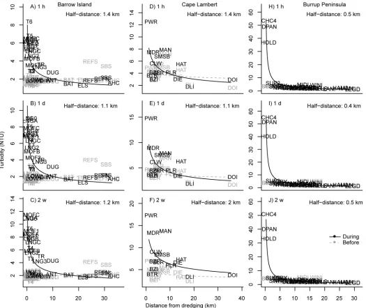
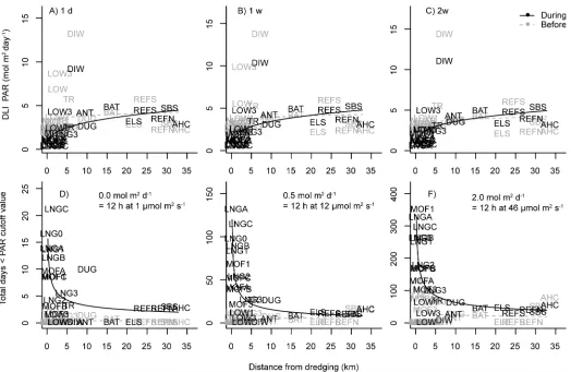
Scatterplots of a range of turbidity (all projects) and light based metrics (Barrow Island only) of water quality clearly indicated a strong power-decay effect with distance from dredging for all three projects, which was absent during the baseline phase (Figs2&3). Distances from dredg-ing effects were apparent in the 80thpercentile values observed across sites during the dredging phase for a range of temporal scales, from 1 h to 2 week running mean turbidity values, with no such spatial patterns apparent prior to dredging (Fig 2). The 80thpercentiles values for tur-bidity decayed rapidly with increasing distance from dredging across all studies, with half-dis-tance values (the dishalf-dis-tances at which turbidity values fell to half of those observed at 200 m of dredging) from just over 1 km for the Barrow Island project (Fig 2A, 2B and 2C), 400 m for Burrup Peninsula project (Fig 2D and 2E) and up to 2 km for the Cape Lambert project (Fig 2H, 2I and 2J). Similar relationships with distance from dredging were also observed for light related water quality metrics at Barrow Island, with DLI values increasing rapidly with increas-ing distance (Fig 3A, 3B and 3C), and the number of observed days at various darkness-cut off levels declining rapidly with distance (Fig 3D, 3E and 3F). Near dredging some sites can experi-ence over 20 days per year where the DLI is near 0 mol photos m-2, over 120 days per year where DLI values are less than 0.5 mol photos m-2and upwards of 340 days per year where DLI levels are less than 2 mol photos m-2(Fig 3).
distances of up to only 2.1 km for the Northern sites at Barrow Island, whereas the Southern sites appeared to show evidence of an effect of distances of up to 20 km (Fig 4,Table 1,S1 File).
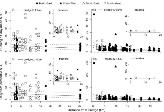
[image:8.612.38.563.76.518.2]Distances from dredging relationships were much weaker for the Cape Lambert and Burrup Peninsula projects (Fig 5,Table 2,S1 File). For the Cape Lambert project, R2values were excep-tionally low (<16% of the variance explained across all metrics) and the best fit models tended to delineate patterns in space rather than an effect of distance to dredging (Fig 5,Table 2A). Baseline data was sparse for the Burrup Peninsula project, as was data at sites very close to the primary dredging activity (S1 Table). What data there is available indicates a potential East/ West interaction during the dredging period, with highly elevated turbidity close to the dredge
Fig 2. Distance decay relationships based on turbidity (80thpercentile NTU) across the three different dredging programs (Barrow Island, Cape Lambert and Burrup Peninsula).Shown are decay relationships based on the 80thpercentile value for each site for the hourly (panels A, D, H), daily (panels B, E, I) and fortnightly (panels C, F, J) running means. Half distance values represent that distance at which each turbidity metric decays to half of the predicted value at 200 m from the dredging activity.
activity for the Western sites, although this relationship is driven by a single point (CHC4, early in 2008). Estimated distances of impact for Burrup Peninsula ranged from 2.1 to 6.0 km, depending on the metric examined (Fig 5,Table 2).
Detailed plume analysis at Barrow Island
The predominantly southerly movement of the dredge plume during the dredging project at Barrow Island, as well as the overall temporal variability in plume extent, can be seen through the sequential time series of the turbidity data across the sites from the north of Barrow Island (the AHC, REFN, ELS, ANT, and LOW sites), through the region of high dredging activity (the MOF and LNG sites) and down through the southern sites (the TR, DUG, BAT, REFS and SBS sites;Fig 6). The time series shows some periods where the turbidity is relatively widespread across many sites, extending to both northern and southern control sites. This is likely to be associated with storm events such as the one occurring in late February associated with tropical cyclone Carlos. At other times the turbidity events are highly contracted, impacting only those sites close to the dredging, and are clearly the result of dredging plumes (Fig 6)
[image:9.612.38.562.74.415.2]The satellite imagery shows that during the dredging period there were clearly visible plumes which generally travelled in a southerly direction, (Fig 7B & 7C). In the July 2010
Fig 3. Distance decay relationships based on light for the Barrow Island dredging program.Shown are distance relationships based on the 20th
percentile of the daily light integral (DLI) value for 1 day (A), 1 week (B) and 2 week running means (C); and the total number of days in near-darkness (normalised to 1 year) for DLI threshold values of ~0 mol m-2photons (D), 0.5 mol m-2photons (E) and 2.0 mol m-2photons (F).
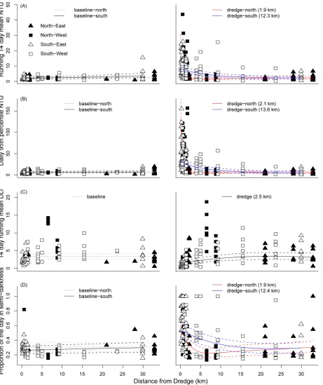
Fig 4. Distance decay relationships for four representative water quality metrics during the Barrow Island project.Shown are: (A) Daily 95th percentile of turbidity, (B) running 14 day mean turbidity, (C) running 14 day mean DLI and (D) proportion of the day below 0.2 DLI. Fitted curves represent fitted best fit Generalised Additive Mixed Models±95% confidence. Baseline and dredge periods were fitted as a two way interaction with distance from dredge, or as a three way interaction as appropriate (North/South or East/West of the location of the primary dredging activity, seemethodsfor further details). Values in parentheses indicate the distance at which the fitted curve falls below the 80thpercentile of the baseline value (i.e. the dredging effect becomes negligible). Data points represent quarterly 95thpercentile values for each site and period (baseline or dredge).
image, the plume was relatively widespread and well mixed, with clear evidence of high sus-pended sediment concentrations near the primary dredging activity as well as at sites as far away as DUG (~9 km, with mean of 9.4 NTU), followed by LNG3 (mean of 7.1 NTU) and LNG1 (mean of 4.3 NTU;Fig 7B & 7E). In the August 2010 image the plume was highly spa-tially complex, and despite being readily apparent on satellite imagery, resulted in only mar-ginal increases in turbidity across the sites (Fig 7F).
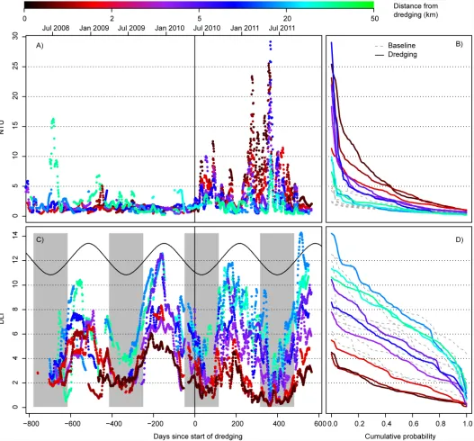
The relatively systematic decline in water quality impacts from dredging across these south-ern sites at Barrow Island can be seen clearly in daily time series data for both turbidity and light across the southern transect of sites at Barrow Island; with very high peaks in turbidity (Fig 8A) and associated declines in light evident throughout the dredging period (Fig 8B). There was a clear shift across this southern transect in terms of the cumulative probability dis-tribution curves for both turbidity (Fig 8C) and light (Fig 8D), with dredging causing a positive shift in turbidity (Fig 8C) and a negative shift in light (Fig 8D) across the full range of
probabilities.
[image:11.612.38.577.156.425.2]The high turbidity during the dredging period resulted in sites close to the dredging activity having DLI levels of<2 mol photons m-2for up to 80% of the time, with values of less than 4 mol photons m-2being relatively commonplace (Fig 8D). There is a clear seasonal pattern in light levels following annual changes in daylight hours, with the low light conditions associated with high turbidity being most pronounced during the already lower light winter months (Fig 8C). Importantly, even for a strongly directionally biased plume such as that seen in the Barrow
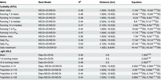
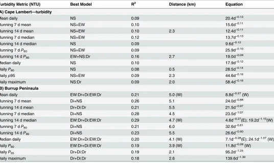
Table 1. Distance from the dredging activity relationships for the Barrow Island project.Shown are results for 11 turbidity (NTU) and 6 light based water quality metrics. The notation ofP80andP95represents the 80thand 95thpercentiles. Shown are the‘best’model as selected by AICc (seemethodsfor
more details), R2values, along with estimated distance of effects and power decay functions (Equation; in the form a*d-b, where d is distance from the primary dredging activity), divided into spatial components (N-S—North or South, E—W–East or West) where required according to the best model. The distance of effect values represent the distance at which the fitted curve falls below the 80thpercentile of the baseline value (i.e. the dredging effect becomes negligible).
Notation for the‘best’model are as follows: NS—a North versus South factor; EW—an East versus West fixed factor; Dr—a factor delineating the pre-dredge versus during dredging; Di—a continuous predictor representing the distance from dredging; Dep—a continuous predictor representing the depth of sites;“:” indicates an interaction among the predictors.
Metric Best Model R2 Distance (km) Equation
Turbidity (NTU)
Mean daily NS:Dr+Di:NS:Dr 0.46 1.9(N); 15.6(S) 11.8d−1.42(N); 12.6d−0.22(S)
Running 7 d mean NS:Dr+Di:NS:Dr 0.48 1.9(N); 15.9(S) 10.3d−1.54(N); 10.8d−0.23(S)
Running 14 d mean NS:Dr+Di:NS:Dr 0.48 1.9(N); 13.2(S) 8.2d−1.32(N); 8.6d−0.23(S)
Running 7 d median NS:Dr+Di:NS:Dr 0.44 2.0(N); 12.4(S) 8.6−1.47(N); 9.1d−0.26(S)
Running 14 d median NS:Dr+Di:NS:Dr 0.47 2.1(N); 10.5(S) 5.8d−0.88(N); 6.9d−0.26(S)
Running 7 dP80 NS:Dr+Di:NS:Dr 0.44 1.8(N); 16.5(S) 15.0d−1.64(N); 15.6d−0.22(S)
Running 14 dP80 NS:Dr+Di:NS:Dr 0.47 1.9(N); 13.3(S) 11.7d−1.39(N); 12.5d−0.25(S)
Median daily NS:Dr+Di:NS:Dr 0.36 1.6(N); 19.6(S) 7.3d−1.64(N); 9.0d−0.12(S)
DailyP80 NS:Dr+Di:NS:Dr 0.46 1.8(N); 15.5(S) 17.3d−1.70(N); 19.1d−0.24(S)
DailyP95 NS:Dr+Di:NS:Dr 0.53 2.1(N); 13.6(S) 37.4d−1.12(N); 33.2d−0.35(S)
Daily maximum EW:Dr+Di:EW:Dr 0.55 1.9(E); 8.8(W) 44.4d−0.52(E); 63.3d−0.54(W)
Light (DLI)
Mean Dep+Dr+Di:Dr 0.40 4.6 1.35d0.28
7 d running mean Dep+Dr+Di:Dr 0.48 3.3 2.02d0.26
14 d running mean Dep+Dr+Di:Dr 0.49 2.6 2.35d0.25
Island project, the effects of dredging appear to decline relatively rapidly with distance, with impacts becoming minimal at distances of around 5 km, and completely indistinguishable from baseline at distances of ~15–20 km (Fig 8).
Discussion
[image:12.612.38.563.73.430.2]This is one of the first published studies to examine in detail the spatial impacts of large scale capital dredging operations in a tropical, coral reef setting. Overall there was strong evidence of a relationship with distance from dredging with all the water quality metrics examined, particu-larly for the dredging program at Barrow Island. The impacts of dredging followed a steep power-law decay relationship, with sites near dredging experiencing much greater changes to water quality than the more distant ones, supporting the use of spatial zoning to manage dredg-ing projects [17,33]. The study has also provided valuable information of water quality condi-tions during large scale capital dredging operacondi-tions, allowing the design of future studies on the
Fig 5. Distance decay relationships for the Cape lambert and Burrup Peninsula dredging projects.Shown are the running 14 day mean turbidity (NTU, A) and daily 95thpercentile of turbidity (B) at Cape Lambert, and the running 14 day mean turbidity (C) and daily 95thpercentile of turbidity (D) at Burrup Peninsula. Fitted curves represent fitted best fit Generalised Additive Mixed Models±95% confidence bounds. Baseline and dredge periods were fitted as a two way interaction with distance from dredge, or as a three way interaction as appropriate (North/South or East/West of the location of the primary dredging activity, seemethodsfor further details). Values in parentheses indicate the distance at which the fitted curve falls below the 80thpercentile of the baseline
value (i.e. the dredging effect becomes negligible).
effects of turbidity on tropical species using environmental relevant or realistic exposure sce-narios (see [61]).
[image:13.612.40.576.155.475.2]How far dredging plumes can travel has important implications for the EIA process and compliance water quality and biological monitoring programs. Recently Evans et al. (2012) visually interpreted MODIS images to map the dredge plume boundaries in the shallow, clear water environment of the Barrow Island project. Their analyses showed that occasionally sedi-ment plumes could be observed over 30 km away from the dredging activities. Such observa-tions define a‘zone of influence’i.e. areas where changes in turbidity can occur, but are not necessarily associated with detectable impacts on the benthic biota. Aerial and satellite images are able to detect very small quantities of suspended material if the turbid water is juxtaposed to clear oceanic water. The blue light scattering from the oceanic water can contrast very strongly with the integrated scattering of sediment and organic material over the water column due to subtle changes in ocean colour. During the EIA process, zones of influence are often pre-dicted (by modelling) and the primary reason is so that authorities can be made aware before-hand of potential social issues such as plumes impacting swimming beaches or marine recreational areas. However, at the outer limits of the zone suspended sediment concentrations
Table 2. Distance from the primary dredging activity relationships. Shown are results for 11 turbidity (NTU) based water quality metrics for the Cape Lambert (A) and Burrup peninsula (B) projects. The notation ofP80andP95represents the 80thand 95thpercentiles. Shown are the‘best’model as selected
by AICc (seemethodsfor more details), R2values, along with estimated distance of effects (Distance) and power decay functions (Equation; in the form a.d-b, where d is distance from the primary dredging activity), divided into spatial components where required according to the best model. The distance of effect values represent the distance at which the fitted curve falls below the 80thpercentile of the baseline value (i.e. the dredging effect becomes negligible).
Nota-tion for the‘best model’are as follows: NS—a North versus South factor; EW—an East versus West fixed factor; Dr—a factor delineating the pre-dredge ver-sus during dredging; Di—a continuous predictor representing the distance from dredging; Dep—a continuous predictor representing site depth;“:”indicates an interaction among the predictors.
Turbidity Metric (NTU) Best Model R2 Distance (km) Equation
(A) Cape Lambert—turbidity
Mean daily NS 0.09 20.4d−0.13
Running 7 d mean NS+EW 0.10 15.6d−0.11
Running 14 d mean NS+EW 0.10 2.3 12.4d−0.11
Running 7 d median NS+EW 0.12 13.7d−0.13
Running 14 d median NS 0.09 9.6d−0.12
Running 7 dP80 NS+EW 0.09 25.9d−0.10
Running 14 dP80 EW+NS:Dr 0.16 2.7 19.0d−0.09
Median daily NS 0.10 17.9d−0.12
DailyP80 NS 0.08 0.5 28.5d−0.14
Dailyp95 NS+EW 0.09 2.3 44.6d−0.16
Daily maximum NS:Dr 0.09 2.0 58.4d−0.16
(B) Burrup Peninsula
Mean daily EW:Dr+Di:EW:Dr 0.21 5.0 (W) 8.8d−0.27(W)
Running 7 d mean Di+NS 0.26 5.1 24.0d−0.88
Running 14 d mean Dr+Di:Dr 0.21 5.5 21.5d−0.97
Running 7 d median Di+NS 0.28 4.5 23.5d−1.07
Running 14 d median EW:Dr+Di:EW:Dr 0.29 4.7 (W) 4.6d−0.27(E); 19.2d−1.15(W)
Running 7 dP80 Di+NS 0.21 6.0 32.6d−0.81
Running 14 dP80 Di+NS 0.23 5.5 26.6d−0.90
Median daily EW:Dr+Di:EW:Dr 0.20 4.1 (W) 7.1d−0.28(E); 24.1d−1.07(W)
DailyP80 EW:Dr+Di:EW:Dr 0.19 3.9 (W) 11.8d−0.28(W)
DailyP95 Dr+Di:Dr 0.19 2.1 95.2d−1.25
Daily maximum Dr+Di:Dr 0.18 2.6 139.6d−1.30
are, by definition, at the limits of the detection techniques, and are likely to be very low and within the range of turbidity naturally experienced during wind and wave events. It is question-able whether such weak plumes will exert any significant biological effects; An unintended con-sequence, however, could be a public misconception of the scale of potential deleterious effects (for further discussion of the issue see [29]).
[image:14.612.39.570.76.541.2]For the purpose of defining the extent of the plume footprint in this study, we used a crite-rion where the value of the fitted curve (representing a median) intersects the 80thpercentile
Fig 6. Turbidity time series for the Barrow Island project.Shown are turbidity (NTU) measured every 10 mins from September 2009 to November 2011 at 25 water quality monitoring sites located from ~30 km north to ~30 km south of the main dredging areas (seeFig 1for sites names and details). Gaps in the data represent occasional failure of the loggers. Each figure is scaled identically from 0–100 NTU. Occasionally readings exceed 100 NTU (see [21] andS1 Tablecontains full, non-truncated summary statistics).
Fig 7. A comparison of satellite images and turbidity.Images are shown for three periods during the Barrow Island dredging program, taken on: (A) 23rd
of November 2008 (baseline phase), (B) 24thof July 2010 (dredging phase), and (C) 29thAugust 2010 (dredging phase). Images from (A) and (C) were
sourced from the Japan Aerospace Exploration Agency (JAXA) Advanced Land Observing Satellite (ALOS) Advanced Visible and Near Infrared Radiometer type 2 (AVNIR-2) satellite. image (10 m pixel resolution). The image in (B) was sourced from the Landsat 5 Thermal Mapper (Path/Rows 114/74-75) 30 m resolution (courtesy of the U.S. Geological Survey)(see alsoFig 1for sites names). Turbidity data (NTU) are shown for the three days surrounding the image date for each image (D, E and F), including all sites for which there were data across all three periods. The grey shaded area indicates the data for the specific date of each image.
(P80) of the baseline value for turbidity (or the 20thpercentile for the light data). This compari-son procedure (P50–P80) has its origins in the Australia and New Zealand water quality guide-lines for fresh and marine waters [59]. The basis is somewhat arbitrary but also pragmatic and associated with a notion of the developers that a median value at an impact site above the 80th percentile of a reference site represents a‘measurable perturbation’, and thus worth investigat-ing [59]. The approach is nevertheless useful as it links water quality with the possibility of
Fig 8. Daily time series and cumulative probability plots.Shown are running 14 day mean turbidity (NTU; A and C) and light (DLI; B and D), with a colour ramp indicating relative distance from dredging activity. Only sites south of the LNG dredging activity (seeFig 4) are included to aid figure clarity. Grey panels indicate the six shortest-day months of the year, based on sun-rise and sun-set data in the region.
ecological change and is also based on a relative change rather than an absolute value [62]. In this study theP50–P80approach was compared to pre-dredging baseline period (as opposed to comparing to control of reference sites) and impacts of dredging on water quality appear to extend distances of ~3 km from the dredging, although in one instance extended as far as 15– 20 km. The larger estimate for potential distances of measurable effect occurred during the Bar-row Island project, where local oceanographic features produced an unusual pattern of a near unidirectional flow southwards over the duration of the project, with minimal days of north-ward movement. This pattern resulted in the significant three-way interaction between the baseline-versus-dredging periods, distance from dredging, and a north versus south characteri-sation of sites. The outcome of interaction was that there was a slower decline of water quality with distance south of the primary dredging area (P50–P80distances of 8.8–19.6 km), with a correspondingly much faster decline in the north (P50–P80distance of 1.5–2.1 km).
Overall the strength of the relationship with distance from dredging was much weaker for the Cape Lambert and Burrup Peninsula projects. The general dredging activity may have been less concentrated given the length of the shipping channels. Both locations are also nearer the mainland and likely to show stronger underlying onshore-offshore gradients in water quality that may have masked patterns associated with dredging. Also, there were much fewer water quality monitoring sites close to the dredging activities in the projects because the regulatory conditions at the time were most concerned with establishing that water quality and ecological change did not occur at more distant sites, than showing effects did occur close to dredging where habitat loss was allowed. This policy direction has recently changed (see [17]).
The spatial analysis carried out here are based on a range of metrics that capture site level summaries across time using a range of temporal scales (hours, days, weeks) and summary metrics (e.g. means, percentiles). However, it is important to remember that such metrics do not necessarily capture the realisedin-situwater quality conditions across all sites at instanta-neous time-scales. While the distance from dredging activity plots may seem relatively consis-tent once poconsis-tential effects of overall plume direction are taken into account, the reality is that at any given time turbidity plumes appear to be highly spatially heterogeneous as clearly shown in the satellite images (Fig 7B & 7C). A peak in turbidity occurring at one location may not be evident at sites only a few hundred metres away. High levels of variation among sites within regions appears to be a consistent feature of turbidity data [63]. Fine scale spatial structure in turbidity raises two issues with respect to dredging management and monitoring that have not yet been thoroughly addressed. First is the issue of whether previously adopted water quality monitoring designs are spatially sufficient, or should more effort be made to establish more optimal designs (e.g. spatially hierarchical and/or stratified sampling [64] or grid sampling [65]) that may be better suited to demonstrating dredging impacts. While power analysis [66–
68], principles of optimal sampling design [64,69–71] and before-after-control-impact
assess-ment [72,73], as well as cost benefit analysis [74] are widespread in ecology, such principles are not often applied to water quality sampling. Second is the issue that if there is poor temporal correlation in water quality readings among sites even at relatively small spatial scales, moni-toring protocols and threshold values based on the use of comparisons to control or reference sites may be of limited value unless extreme care is taken to ensure they adequately represent the impact locations [39].
that was spatially designed for looking at effects of distance from the placement sites, rendering the conclusion of such analyses relatively weak. The effect of the disposal at Barrow Island can be seen in the satellite images inFig 7B & 7C(bottom left hand corner of enlarged panels), and generally appears relatively minor compared to the turbidity generated at the point of excava-tion. For the Barrow Island project the spoil disposal site was situated to the south east of the dredging activities and may in fact partially account for some of the southerly extent of the Bar-row Island dredge plume. In this context the distance analysis reported here potentially repre-sents the total effect of the whole dredge operation (both excavation and disposal), with anything over ~15–20 km not affected.
Water Quality thresholds for reef biota
TheP50–P80approach of ANZECC/ARMCANZ to estimate distances of detectable effects is recommended where information on biological responses is absent, and is considered to be rea-sonably conservative. Other statistical criteria based on water quality could be used, that might yield substantially different estimated distances. For example, it could be defined as the dis-tance at which the predicted (best fit value, representing a mean or median) crosses the upper 95thpercentile value of the baseline state. Such a definition would likely yield shorter distances of potential impact than currently reported here.
What is really needed to define the distance of effects are water quality thresholds which relate changes in the physical parameters (light reduction, total suspended sediment, sediment deposition) to biological responses (sublethal and lethal) of the underlying organisms. Such thresholds are not yet available for reef biota such as coral, seagrasses and filter feeders and require laboratory and/or manipulative field based studies and subsequent verification before being used. The spatial analyses described here and the temporal analyses described in Jones et al. [21] have however provided some insights into the problems that need to be addressed when developing such thresholds, and especially how to incorporate exposure across varying temporal scales. For example, during the Barrow Island project,>50% of the daily light inte-grals were very low (i.e.<1.5 mol photons m-2) at sites within a few hundred metres of the dredging, as opposed to 3–8 mol photons m-2during the baseline period. Clearly light was affected by dredging but it is very significant for the underlying communities whether these low light values occur at once or intermittently. Theoretically, an intermittent pattern could afford the opportunity for primary producers such as corals to recover energy deficits between the low light periods. This has already been suggested as a mechanism for how corals survive natural resuspension events ([9,75]). Simple inspection of the data shows many low light days occurred in a near continuous block in the winter period, where a combination of low seasonal light availability and more intense turbidity generating events resulted in a 6 month period of DLIs<1 mol photons m2. The pattern suggests one possible management practice could be timing maintenance and/or short-term capital dredging programs to avoid seasonal lows in light availability if light is considered a key pressure parameter (i.e. dredging near seagrass beds). However the data also suggests that analyses of water quality data using the whole dredg-ing or baseline periods usdredg-ing cumulative probability plots (seeFig 8) although instructive for characterizing effects on a broad scale, is much too coarse for threshold development.
in terms of distance from the dredging activities (this study) has provided a matrix of environ-mentally realistic exposure conditions that can be used to explore lethal and sub-lethal water quality thresholds in future laboratory- and field-based manipulative studies (see onlineS1 Table). This could ultimately lead to a more accurate definition of the potential ecological foot-print of plumes from dredging projects than theP50–P80approach used here or other statistical approaches.
The three projects described here spanned a range of environmental settings including an offshore,‘clear water’environment (Barrow Island), an exposed nearshore cape or headland (Cape Lambert), and an enclosed inshore turbid reef environment (Mermaid Sound, Burrup Peninsula). Nevertheless, the patterns of turbidity generation will be highly site and project specific and will vary with production rates (volumes dredged) and dredge types (cutter suction dredge versus back hoe or TSHD) and methodology used (overflow etc). Other factors include the nature of the sediments being dredged and the oceanographic conditions such as tidal and current strengths and wind- and wave-induced resuspension associated with seabreezes. For the upper (15–20 Km) bound identified for the Barrow Island project, it should be recognized that was a very large scale capital dredging operation (8 Mm3) with multiple dredges working 24 a day, in a clear water environment, and with the unusual oceanographic feature of unidirec-tional flow. As such, we consider that the southerly extension of the plume represents an upper bound on the distances at which dredging might be expected to cause‘measurable perturba-tions’as defined by theP50–P80approach.
Supporting Information
S1 File. Detailed results.Full subsets best model output (Tables A-C) and plotted best model fits (Figures A-D) for all variables examined statistically for distance decay relationships for each of the three dredging projects in the Pilbara.
(PDF)
S1 Table. Detailed summary data.Max, 99th, 95th, 80th percentiles, median and mean NTU values over 1 h, 1 d, 14 d, and 21 d running average period at all sites during the baseline period or for during the duration of the dredging program.
(PDF)
Acknowledgments
We thank industry for making this data available for scientific research and M. Poutinen for providing information on cyclone activity.
Author Contributions
Conceived and designed the experiments: RF RJ CS PR. Analyzed the data: RF RJ CS. Wrote the paper: RF RJ PR CS.
References
1. Bray RN (2008) Environmental aspects of dredging. CRC Press.; Bray RN, editor.
2. Johnston JSA (1981) Estuarine dredge and fill activities: a review of impacts. Environmental Manage-ment 5: 427–440.
3. Newell R, Seiderer L, Hitchcock D (1998) The impact of dredging works in coastal waters: a review of the sensitivity to disturbance and subsequent recovery of biological resources on the sea bed. Ocean-ography and Marine Biology: An Annual Review 36: 127–178.
5. Thrush SF, Dayton PK (2002) Disturbance to marine benthic habitats by trawling and dredging: implica-tions for marine biodiversity. Annual Review of Ecology and Systematics 2002: 449–473.
6. Morton J (1977) Ecological effects of dredging and dredge spoil disposal: A literature review. US Fish and Wildlife Service Technical Papers 94: 1–33.
7. Jones R, Ricardo GF, Negri AP (2015) Effects of sediments on the reproductive cycle of corals. Marine Pollution Bulletin doi:10.1016/j.marpolbul.2015.08.021
8. Kleypas JA, McManus JW, Meñez LA (1999) Environmental limits to coral reef development: where do we draw the line? American Zoologist 39: 146–159.
9. Anthony KR, Fabricius KE (2000) Shifting roles of heterotrophy and autotrophy in coral energetics under varying turbidity. Journal of experimental marine biology and ecology 252: 221–253. PMID:
10967335
10. Bak RPM (1978) Lethal and sublethal effects of dredging on reef coral. Marine Pollution Bulletin 9: 14– 16.
11. Rogers CS (1990) Responses of coral reefs and reef organisms to sedimentation. Marine Ecology Progress Series 62: 185–202.
12. Erftemeijer PL, Lewis RRR (2006) Environmental impacts of dredging on seagrasses: A review. Marine Pollution Bulletin 52: 1553–1572. PMID:17078974
13. Erftemeijer PLA, Riegl B, Hoeksema BW, Todd PA (2012) Environmental impacts of dredging and other sediment disturbances on corals: A review. Marine Pollution Bulletin 64: 1737–1765. doi:10. 1016/j.marpolbul.2012.05.008PMID:22682583
14. Doorn-Groen SM, Foster T (2007) Environmental monitoring and management of reclamations works close to sensitive habitats. Terra et Aqua 108: 3.
15. Trimarchi S, Keane J (2007) Port of Hay Point Apron Areas and Departure Path Capital Dredging Proj-ect. Environmental Review, EcoPorts Monograph Series 24.
16. Foster T, Corcoran E, Erftemeijer P, Fletcher C, Peirs K, Dolmans C, et al. (2010) Dredging and port construction around coral reefs. PIANC Environmental Commission, Report No 108.
17. EPA (2011) Environmental Assessment Guidleine for Marine Dredging Programs EAG7. Perth, West-ern Australia: Environmental Protection Authority (EPA). pp. 36.
18. Hanley JR (2011) Environmental monitoring programs on recent capital dredging projects in the Pilbara (2003–10): a review. APPEA J: 273–294.
19. Wolanski E, Gibbs R (1992) Resuspension and clearing of dredge spoils after dredging, Cleveland Bay, Australia. Water environment research 1992: 910–914.
20. McArthur C, Ferry R, Proni J. (2002) Development of guidelines for dredged material disposal based on abiotic determinants of coral reef community structure. Proceedings of the third Speciality Conference on Dreding and Dredged Material Disposal Coasts, Oceans, Ports and Rivers Institute (COPRI) of ASCE. Orlando, FL, USA. 1–15.
21. Jones R, Fisher R, Stark C, Ridd P (2015) Temporal patterns in water quality from dredging in tropical environments. PlosOne 10: e0137112.
22. Koskela RW, Ringeltaube P, Small AR, Koskela TV, Fraser AR, Lee JD, et al. (2002) Using predictive monitoring to mitigate construction impacts in sensitive marine environments 10th Pacific Congress on Marine Science and Technology (PACON 2002) July 21–26, 2002, Chiba, Japan
23. Stoddart J, Anstee S (2004) Water quality, plume modelling and tracking before and during dredging in Mermaid Sound, Dampier, Western Australia. Corals of the Dampier Harbour: their survival and repro-duction during the dredging programs of 2004: 9–30.
24. VBKO (2003) Protocol for the Field Measurementof Sediment Release from Dredgers. A practical guide to measuring sediment release from dredging plant for calibration and verification of numerical models. Reporrt produced for VBKO TASS project by HR Wallingford Ltd & Dredging Research Ltd Issue 1:83 pp.
25. Van Der Veer HW, Bergman MJN, Beukema JJ (1985) Dredging activities in the Dutch Wadden Sea: effects on macrobenthic infauna. Netherlands Journal of Sea Research 19: 183–190.
26. Nichols M, Diaz R, Schaffner LC (1990) Effects of hopper dredging and sediment dispersion, Chesa-peake Bay. Environmental Geology and Water Sciences 15: 31–43.
27. Hitchcock D, Bell S (2004) Physical impacts of marine aggregate dredging on seabed resources in coastal deposits. Journal of Coastal Research 20: 101–114.
29. Spearman J (2015) A review of the physical impacts of sediment dispersion from aggregate dredging. Marine Pollution Bulletin 94: 260–277. doi:10.1016/j.marpolbul.2015.01.025PMID:25869201
30. Ruffin K (1998) The persistence of anthropogenic turbidity plumes in a shallow water estuary. Estua-rine, Coastal and Shelf Science 47: 579–592.
31. Fredette T, French G (2004) Understanding the physical and environmental consequences of dredged material disposal: history in New England and current perspectives. Marine Pollution Bulletin 49: 93– 102. PMID:15234878
32. Cutroneo L, Castellano M, Pieracci A, Povero P, Tucci S, Capello M (2012) The use of a combined monitoring system for following a turbid plume generated by dredging activities in a port. Journal of Soils and Sediments 12: 797–809.
33. GBRMPA (2012) The use of hydrodynamic numerical modelling for dredging projects in the Great Bar-rier Reef Marine Park, Great BarBar-rier Reef Marine Park Authority, Townsville. GBRMPA External Guide-line. In: GBRMPA (ed), Townsville (Queensland, Australia).
34. Mulligan M (2009) 'Applying the learning' The Geraldton Port dredging project 2002–03. Paper to the Freight and Logistics Council of WA and Ports WA—1st of December 2009 Mulligan Environmental, Western Australia.
35. CEDA (2015) Environmental Monitoring Procedures. Information paper. Central Dredging Association (CEDA) Delft The Netherlands (http://www.dredging.org/media/):23 pp.
36. McCook L, Schaffelke B, Apte S, Brinkman R, Brodie J, Erftemeijer P, et al. (2015) Synthesis of current knowledge of the biophysical impacts of dredging and disposal on the Great Barrier Reef: report of an independent panel of experts.
37. Larcombe P, Costen A, Woolfe KJ (2001) The hydrodynamic and sedimentary setting of nearshore coral reefs, central Great Barrier Reef shelf, Australia: Paluma Shoals, a case study. Sedimentology 48: 811–835.
38. Larcombe P, Ridd PV, Prytz A, Wilson B (1995) Factors controlling suspended sediment on inner-shelf coral reefs, Townsville, Australia. Coral Reefs 14: 163–171.
39. Orpin A, Ridd P, Thomas S, Anthony K, Marshall P, Oliver J (2004) Natural turbidity variability and weather forecasts in risk management of anthropogenic sediment discharge near sensitive environ-ments. Mar Pollut Bull 49: 602–612. PMID:15476839
40. Orpin AR, Ridd PV (2012) Exposure of inshore corals to suspended sediments due to wave-resuspen-sion and river plumes in the central Great Barrier Reef: A reappraisal. Continental Shelf Research 47: 55–67.
41. Bivand R, Keitt T, Rowlingson B (2015) rgdal: Bindings for the Geospatial Data Abstraction Library. R package version 1.0–7.http://CRAN.R-project.org/package = rgdal.
42. Geoscience Australia (2004) Geodata Coast 100K 2004. Geoscience Australia, Canberra.<http:// www.ga.gov.au/>.
43. Murrell P (2014) gridBase: Integration of base and grid graphics. R package version 0.4–7.http:// CRAN.R-project.org/package = gridBase.
44. Adobe Illustrator (2012) (Version CS6) [Computer software]. San Jose, CA: Adobe Systems Incorporated.
45. Wood SN (2006) Generalized Additive Models: an introduction with R. Boca Raton, FL: CRC Press. 410 p.
46. R Core Team (2014) R: A language and environment for statistical computing. R Foundation for Statis-tical Computing, Vienna, Austria. URLhttp://www.R-project.org/.
47. Tuszynski J (2013) caTools: Tools: moving window statistics, GIF, Base64, ROC AUC, etc. R package version 116http://CRANR-projectorg/package = caTools.
48. Zeileis A, Grothendieck G (2005) zoo: S3 Infrastructure for Regular and Irregular Time Series. Journal of Statistical Software 14: 1–27.
49. Wood S, Scheipl F (2013) gamm4: Generalized additive mixed models using mgcv and lme4. R pack-age version 0.2–2.http://CRANR-projectorg/package = gamm4.
50. ESRI (2013) ArcGIS Desktop, v10.2. Redlands CA, Environmental Systems Research Institute.
51. Carroll SS, Pearson DE (2000) Detecting and modeling spatial and temporal dependence in conserva-tion biology. Conservaconserva-tion Biology 14: 1893–1897.
52. Cryer JD, Chan K-S (2008) Time series regression models. Time series analysis: with applications in R. pp. 249–276.
54. Kirk JT (1985) Effects of suspensoids (turbidity) on penetration of solar radiation in aquatic ecosystems. Perspectives in Southern Hemisphere Limnology. Springer.
55. Cavanaugh JE (1997) Unifying the derivations of the Akaike and corrected Akaike information criteria. Statistics & Probability Letters 31: 201–208.
56. Burnham KP, Anderson DR (2002) Model Selection and Multimodel Inference; A Practical Information-Theoretic Approach. New York: Springer. 488 p.
57. Bates DM, Watts DG (1988) Nonlinear Regression Analysis and Its Applications, Wiley
58. Bates DM, Chambers JM (1992) Nonlinear models. Chapter 10 of Statistical Models in S. In: Hastie JMCaTJ, editor: Wadsworth & Brooks/Cole.
59. ANZECC/ARMCANZ (2001) Australian and New Zealand guidelines for fresh and marine waters. Aus-tralian and New Zealand Environment and Conservation Council & Agriculture Resource Management Council of Australia and New Zealand, Canberra.
60. Evans RD, Murray KL, Field SN, Moore JAY, Shedrawi G, Huntley BG, et al. (2012) Digitise This! A Quick and Easy Remote Sensing Method to Monitor the Daily Extent of Dredge Plumes. PLoS ONE 7: e51668. doi:10.1371/journal.pone.0051668PMID:23240055
61. Harris CA, Scott AP, Johnson AC, Panter GH, Sheahan D, Roberts M, et al. (2014) Principles of Sound Ecotoxicology. Environmental Science & Technology 48: 3100–3111.
62. Fox D (2001) Understanding the new ANZECC Water Quality Guidelines.http://www.environmetrics.
net.au/docs/THE%20NEW%20ANZECC%20WATER%20QUALITY%20GUIDELINES_2_.pdf.
63. Macdonald RK, Ridd PV, Whinney JC, Larcombe P, Neil DT (2013) Towards environmental manage-ment of water turbidity within open coastal waters of the Great Barrier Reef. Mar Pollut Bull 74: 82–94. doi:10.1016/j.marpolbul.2013.07.026PMID:23948091
64. Andrew NL, Mapstone BD (1987) Sampling and the description of spatial pattern in marine ecology. Oceanography and Marine Biology: an annual review 25: 39–90.
65. Cole RE, H T.R., Wood ML, Foster DM (2001) Statistical analysis of spatial pattern: a comparison of grid and hierarchical sampling approaches. Ecological Monitoring and Assessment 69: 85–99.
66. Osenberg CW, Schmitt RJ, Holbrook SJ, Abu-Saba KE, Flegal AR (1994) Detection of Environmental Impacts: Natural Variability, Effect Size, and Power Analysis. Ecological Applications 4: 16–30.
67. Gerrodette T (1987) A power analysis for detecting trends. Ecology 1987: 1364–1372.
68. Fairweather PG (1991) Statistical power and design requirements for environmental monitoring. Marine and freshwater research 42: 555–567.
69. Chapman MG (1999) Improving sampling designs for measuring restoration in aquatic habitats. Journal of Aquatic Ecosystem Stress and Recovery 6: 235–251.
70. Block WM, Franklin AB, James P. Ward J, Ganey JL, White GC (2001) Design and implementation of monitoring Studies to evaluate the success of ecological restoration on wildlife. Restoration Ecology 9: 293–303.
71. Millard SP, Lettenmaier DP (1986) Optimal design of biological sampling programs using the analysis of variance. Estuarine, coastal and shelf science 22: 637–656.
72. Green RH (1979) Sampling design and statistical methods for environmental biologists. New York, USA: Wiley.
73. Underwood AJ (1994) On beyond BACI: sampling designs that might reliably detect environmental dis-turbances. Ecological applications 4: 3–15.
74. Hanley N, Spash CL (1993) Cost-benefit analysis and the environment. Vol. Hanley, Nick, and Clive L. Spash. Cost-benefit analysis and the environment. Vol. 499. Cheltenham: Edward Elgar, 1993. Chel-tenham: Edward Elgar.
75. Anthony K, Larcombe P (2000) Coral reefs in turbid waters: sediment-induced stresses in corals and likely mechanisms of adaptation. Proceedings of the 9thInternational Coral Reef Symposium Bali,