An auto TCD probe design and visualization

Yi Huang1_{, Paul Wen}1_{, Bo Song}2 _{and Yan Li}2

1 _{School of Mechanical and Electrical Engineering, Faculty of Health, Engineering and} Sciences, University of Southern Queensland, Toowoomba, Qld., Australia 2 _{School of Agricultural, Computational and Environmental Sciences, Faculty of Health,} Engineering and Sciences, University of Southern Queensland, Toowoomba, Qld., Australia [email protected] {Paul.Wen,Bo.Song,Yan.Li} @usq.edu.au

Abstract. Transcranial Doppler ultrasound (TCD) is a non-invasive ultrasound method used to examine blood circulation within the brain. During TCD, ultrasound waves are transmitted through the tissues including skull. These sound waves reflect off blood cells moving within the blood vessels, allowing the radiologist to interpret their speed and direction. In this paper, an auto TCD probe is developed to control the 2D deflection angles of the probe. The techniques of Magnetic Resonance Angiography (MRA) and Magnetic Resource Imagine (MRI) have been used to build the 3D human head model and generate the structure of cerebral arteries. The K-Nearest Neighbors (KNN) algorithm as a non-parametric method has been used for signal classification and regression of corresponding arteries . Finally, a global search and local search algorithms are used to locate the ultrasound focal zone and obtain a stronger signal efficient and more accurate result.

Keywords: Auto TCD Probe, K-nearest Neighbor, Signal Search and Classification.

1

Introduction

Transcranial Doppler ultrasound (TCD) is the non-invasive ultrasound technique, which was first described in 1982 [1, 8]. The function of TCD is to monitor cerebral blood flow velocity (CBF-V) and vessel pulsatility [5]. The system of TCD is inexpensive and repeatable for using. Also, it is possible to use for continuous bedside monitoring of CBF-V, which has a positive effect on using in the intensive care [4].

This paper aims to design and develop a freehand auto TCD probe, which can sweep and search brain blood vessels automatically without human intervention. In this study, efficient algorithms to detect and track blood flow signals are proposed with 3D outputs in visualization. In addition, the proposed algorithms drive each small ultrasound transducers independently for better accuracy.

2

Methodology

2.1 Auto Probe Design

The ultrasound probe is made up of two major components. One is the Doppler ultrasound probe, which used the 2 MHz transmission frequency to emit the ultrasound waves from the transducers. The ultrasound probe used in this study is a one dimension ultrasound transducer and there is only one ultrasound wave emitted for each time. The ultrasound transducer connected with two micro motors (motor X and motor Y) by two poles. The two motors control the deflection angles at x and y axis and z axis is the direction of ultrasound waves. The other part is the probe headset, which keeps the probe to the proper position in the temporal ultrasound window. Therefore, the patient can wear the headset in a comfortable state and the clinicians can do the constant monitoring instead of holding the ultrasound probe to measure the blood flow velocity all the time.

The frequency of ultrasound probe utilized in this study is 2 MHz, which can provide the deeper of the ultrasound waves, over 80 mm, because of a lower degree of attenuation [7]. In this study, only left, transtemporal window is used to perform the signal scanning because the Circle of Willis is generally symmetric in theory. For one side of the cerebral arteries, the range of depth 80 mm can be covered the area from the ultrasound window to the middle of the cerebral artery [6].

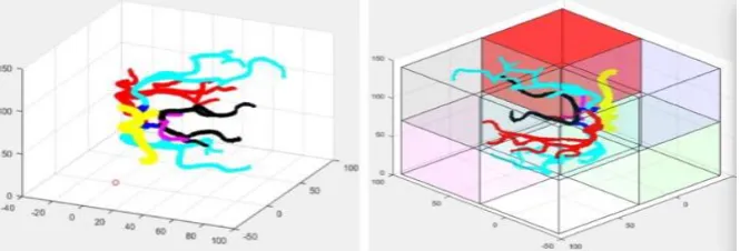
In order to explore the influence of sampling depths, the ultrasound sampling depths in the same direction varies starting from 40 to 80 mm with an incremental setting of 5 mm (as shown in Fig.1). In addition, the deflection angles of each micro motor is configured as 1 degree while the range is between -70 and +70 degrees and the increment of the angles each time is 1 degree. For the direction of x and y poles, there are both 141 cases and the total cases are 141 × 141 = 19881.

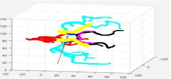
Fig. 2. All scanning area at sampling depths from 40 mm to 80 mm with half side of the circle of Willis.

Fig.2.A demonstrates the scanning area of the ultrasound probe. The red point is the place of the ultrasound probe, the irregular lines are the Circle of Willis and some parts have been covered by the scanning area. The Fig.2.B displays the nine scanning area after zooming in and from the bottom to the top, the sampling depths of ultrasound waves has been increased from 40 mm to 80 mm.

Overall, the designed ultrasound probe can meet the requirements of scanning. Firstly, the sampling depth of ultrasound waves can reach over 80 mm by using the 2 MHz ultrasound transducer, which satisfies the distance from the ultrasound window to the middle cerebral artery. Secondly, using two micro motors with two poles connected to the transducer can easily change the deflection angles of the ultrasound waves and the driving routine is repeatable. Thirdly, the scanning range is large enough, which can cover the half area of the Circle of Willis by using one side of the ultrasound probe.

2.2 Global Search and Algorithm

The global search is to use the ultrasound probe to scan the area of the Circle of Willis within our brains and identify the targeted blood vessel sections. According to the MRI and MRA techniques, it is possible to obtain the data of the corresponding position of each cerebral artery, and then using the finite element method (FEM) to acquire the accurate location of each artery, including the locations in the ultrasound window of a skull. The location of the ultrasound window is the position where placed the ultrasound probe.

Firstly, it is necessary to process the FEM data and do coordinates origin translation. The origin (0, 0, 0) of the original FEM data is predefined as the starting pixel of the MRI volume and this point is later translated to the center of the left ultrasound window. To be specific, there are 118 FEM points of left ultrasound window. The equation 1 to 3 are the average evaluations for the location of x, y and z axis, and the central point that obtained is (120.5096, 122.0414, 162.3302).

𝑥0=𝑥1+ 𝑥2+𝑥₁₁₈3+ ⋯ + 𝑥118

𝑦0=𝑦1+ 𝑦2+𝑦₁₁₈3+ ⋯ + 𝑦118

(1)

𝑧0 =𝑧1+ 𝑧2+𝑧₁₁₈3+ ⋯ + 𝑧118

Secondly, after obtaining the central point of the ultrasound window, the next step is to change the origin of coordinates. While doing the coordinate transformation, the key point is to find the vector of the conversion. The conversion vector is (𝑥0, 𝑦0, 𝑧0) and

all locations of arteries need to be transformed based on the conversion vector. Then, the new location of each artery can be acquired based on the origin of coordinates of the ultrasound window.

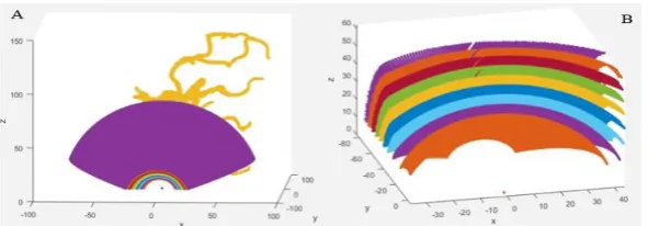
Thirdly, set the sampling depth of ultrasound waves and offset the X and Y micro motors, which can control the reflection angles of transmission. Between the ranges of deflection angles, the angle increment of each time is one degree. So, there are 141 deflection angles for each motor and the total cases of ultrasound wave are 141x141 (19981). Fig.3 displays the yellow curve which consists of 19981 detected signal points.

Fig. 3. Global search based on the sampling depth of ultrasound wave is 50 mm.

The outcome of a global search is to locate the ultrasound focal zone. After the global search for the area of the Circle of Willis at a certain depth, the closest point in the space can be found by using k-nearest neighbor search (KNN) algorithm, which is an optimization method to find the nearest point in the scale space. The echo ultrasound signals are generally stronger when the ultrasound wave is closer to the near arteries. Calculating the Euclidean distance (equation 4) between the detected ultrasound signals and the near sample points of arteries is an efficient method to determine the strength of signals. There are twelve arteries constructed by a total of 10597 FEM points in this study.

𝑑 = √∑𝑘=1𝑛 (𝑥1𝑘− 𝑥2𝑘)2

Applying the KNN algorithm, the k value is set as 10, which means there are 10 neighbor points to the detected signals should be calculated. For the 19881 detected signals, there are 198810 neighbor points calculated in total. The calculation is based on each point of detected signals to their corresponding 10 closest points. According to all values, the next step is to find the minimum distance between test signals and (3)

samples from all the scanning signals. The result obtained is 3813. From the 19881 detected signals, the number of 3813 signal has a corresponding 10 closest signals at the sampling depth of ultrasound wave is 50 millimeters.

2.3 Local Search Approach

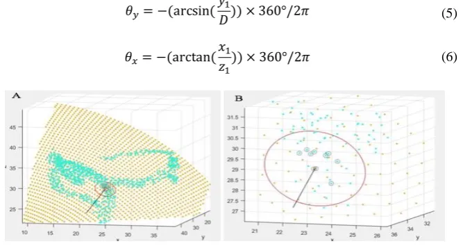
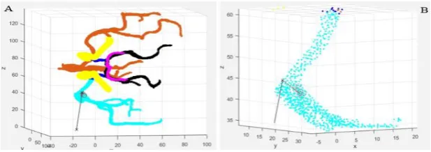
The local search is performed after the global search, which helps to improve the accuracy of searching outputs. In Fig.4, the yellow dots represent the detected signals by global search, and the intensive light blue dots display one of the arteries in the Circle of Willis. The black straight line is the ideal path of the ultrasound wave. The symbol ‘x’ with red color is the accurate scanning point, and it is from the 3813 points calculated by the global search. The small black circles are 10 closest sample signals around the detected signal and the big red circle is the scanning area for the local search. From the global search, the coordinate point of the 3813th detected signal (𝑥1=

22.5133,𝑦1= 34.0999, 𝑧1= 28.8157). Then, the deflection angle of this detected

signal can be calculated in equation 5 and 6. 𝜃𝑦= −43°, 𝜃𝑥= −38°.

𝜃𝑦= −(arcsin(

𝑦1

𝐷)) × 360°/2𝜋

𝜃𝑥= −(arctan(

𝑥1

𝑧1)) × 360°/2𝜋

Fig. 4. Local search based on the sampling depth of ultrasound wave is 50 mm.

Once getting the deflection angle of the strongest detected signal, the local search can start. The sampling depth of the ultrasound probe is still at 50 mm and changing the deflection angles of 𝜃𝑥 and 𝜃𝑦, and the increment of the deflection angle of X and Y

motors is 1 degree. The scanning area is in a circle with the point of (𝑥1, 𝑦1, 𝑧1) as the

center point. Using KNN to search for the nearest 10 neighbor points. According to the obtained signal points to calculate the distance between the points and the Circle of Willis. Using the equation 4 to calculate the Euclidean distance of the nearest 10 neighbor points and matching these points to their corresponding arteries. From the Fig.4, it is obvious that these 10 neighbor points are all in the big red circle of the local search.

The purpose of the local search is to acquire the continuous and stable signal (5)

spectrum. When doing the global search, the signal image is intermittent, unless continuous signals are detected from certain areas. When acquiring the strong signal from the global search, it is not easy to determine that the nearby search area of signal points can output stable and continuous signal images. The suitable scanning area might improve the accuracy of outputs and the signal image on the Doppler ultrasound system can be more clearly, which has a positive effect on understanding the index and parameters of ultrasound for diagnosis. Furthermore, when a patient coughs during the process of operation, a false strong signal might be produced and output on the Doppler ultrasound system. The system may misinterpret the false signal as the strongest signal after finishing the global search. Therefore, it cannot search any signals at that certain area during the process of local search and also it cannot display stable and continuous signals on the Doppler ultrasound system. As a result, local search is an efficient method to examine the true or false strong signals from global search.

2.4 Signal Classification and Implementation

The method used for the signal classification is the K-Nearest Neighbor (KNN). In the KNN classification, the output is determined by the "majority vote" of its neighbor, and the most common classification of the nearest neighbor determines the category to which the object is assigned [2]. If k = 1, the object's class is given directly by the nearest node [10]. The first step of the KNN algorithm is to calculate the distance between the detected signal and each training data and then sorting the data according to the increasing relation of distance. The second step is to select K points with the smallest distance and then determining the occurrence frequency of the category of the first K points. The last step is to return the category with the highest frequency in the K points before as the prediction classification of test data.

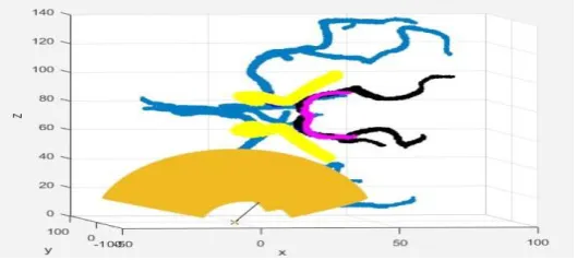
Fig. 5. Circle of Willis and divided into eight regions.

color represents the middle cerebral artery (MCA) and the pink color displays superior cerebellar artery (SCBA). The Circle of Willis has been divided into eight regions in Table.1.

Table 1. The arteries are divided into eight regions

Region The corresponding arteries in the region Red RICA,RMCA,LPCA,RPCA,LSCBA,RSCBA Blue LACA,RACA,RCOA,RICA,RMCA,RPCA Yellow LCOA,LICA,LMCA,LPCA,LSCBA,RSCBA

Green LACA,RACA,LCOA,LICA,LMCA,LPCA

Black RACA,RMCA

Light Blue LACA,RACA,RMCA

Pink LACA,LMCA,LPCA

White LACA,LMCA

The advantage of dividing the Circle of Willis into eight regions is reducing the amount of calculation and it is also more convenient to classify the signal data. After setting the sampling depth of the ultrasound wave and the deflection angles of X and Y motors, it can be classified as the signal to its corresponding region (Table.2).

Table 2. Classify random signals.

Depth (mm)

Deflection angle (X)

Deflection angle (Y)

Region

45 -5 -10 Green

60 15 10 Green

50 5 -45 White

55 -30 -20 Yellow

70 25 45 Non

There are two ways to classify the signals to their corresponding arteries. Global classification (Fig.6) is to use scanning signal to calculate the distance between each artery and all detected signals, which is very computationally intensive.

Fig. 7. Local classification. Sampling depth at 45 mm and deflection angles are -10 and -5.

For the local classification (Fig.7), the first step is to estimate the location of the detected signal. When the sampling depth of the ultrasound wave is 45 mm and the deflection angles are -10 and -5, the detected signal is in the green region. From Table.1, there are six cerebral arteries in the green region. Compared with the global classification, it is necessary to calculate the distance of the six arteries instead of all twelve arteries with the detected signal, which has a positive effect on reducing the calculations in half.

The important step when doing the signal classification is to calculate the ration of closest points from all of 10 points to each artery. In Fig.6 and 7, all 10 closest points are from the same artery, LMCA. As a result, the detected signal can be classified to LMCA.

Fig. 8. Local classification. Sampling depth at 62 mm and deflection angles are -10 and -8

3

Results

3.1 Analyzing the data

The Table.3 displays the signals classification based on the global search and the local search at the sampling depths varying from 40 mm to 80 mm for only the left side of ultrasound transmission and the K value is 10.

Table 3. Classifies the detected signals varying the sampling depth from 40 mm to 80 mm.

Depth (mm) Classify the signal to Artery

40 LMCA

45 LMCA

50 LMCA

55 LMCA

60 LICA

65 LACA

70 LPCA

75 LACA

80 LSCBA

To verify the results above, the K value is selected from 10 to 5 and 15

Fig. 9. Sampling depth at 45 mm and K values are 5 and 15.

Fig. 10. Sampling depth at 62 mm and deflection angles are -8 and -10. K=3, 5, 10 and 20.

To evaluate the effect of K value on classification results. The sampling depth of the ultrasound wave is selected as 62 mm and the K values are changed from 3 to 5, 15 and 20 ( Fig.10 to 13). When K=3, there are two sample points from LCOA and only one point is from LICA. Therefore, the detected signal belongs to LCOA. When K=5, there are both 2 sample points from LMCA and LCOA and only one point is from LICA. However, the distance between the detected signal and the sample points of LCOA is shorter than the sample points of LMCA. As a result, the detected signal should be classified to LCOA. When K=15, there are 7 sample points from LCOA and there are 3 and 5 sample points from LICA and LMCA respectively. The signal classification of the detected signal is to LCOA as well. When K=20, there are 10 sample points from LCOA and there are both 5 sample points from LICA and LMCA. The signal classification results from above are LCOA when the K value is different.

3.2 Findings

Table 4 shows the characteristic of cerebral vasculature, including the sampling depth of cerebral arteries, which helps to compare the data accuracy.

Table 4. Characteristics of cerebral vasculature (Naqvi et al., 2013)

Artery Depth (mm) Adult MFV(cm/s)

LMCA 30-65 55±12

LACA 60-75 50±11

LPCA 60-70 40 ± 10

LCOA 45-55 21 ± 5

LICA 65-80 41 ± 15

LSCBA 80-12 41 ± 10

Compared the Table.3 and Table.4, at the sampling depths of ultrasound waves are 40,

A B

45, 50, 55, 65, 70, 75 and 80, the signals classification results are consistent with the data obtained in Table.4. At the sampling depth of ultrasound wave is 60 mm, the classification of the detected signal is belong to the LICA, which is different with the obtained data in Table 4 (the depth of LICA is between 65 and 80 mm). To verify the accuracy of the comparison, a number of random and irregular sampling depths, such as 52, 57 and 63 are selected as shown in Table.5.

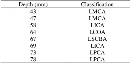
Table 5. Classify the detected signals at random sampling depths

Depth (mm) Classification

43 LMCA

47 LMCA

58 LICA

64 LCOA

67 LSCBA

69 LICA

73 LPCA

78 LPCA

Table 5 demonstrates the classification results at the random sampling depths of detected signals. Compared with Table 4 and 5, it is easy to find that the results from the experiment are not consistent with the obtained data and biased, such as the classification results of LPCA and LSCBA.

3.3 Discussion of result

Firstly, there are some regular parameters, such as depth, have been set to test the outputs of the experiment, and the results and expectations are consistent. Also, some specific parameters have to test the accuracy of classification results. For example, different values of k are chosen, such as 3, 5 and 20, to search the number of K nearest sample points to the detected signals and according to the proportion of sample numbers to classify the signals. In some specific cases, the sample points distributed into different arteries. The classification results of the artery have been determined by the higher proportion of the sample points.

4

Conclusion

During the TCD, it is difficult to pin point and hold the ultrasound probe to the right direction manually, which is experience-dependent and time-consuming. This study proposed and developed an auto TCD probe, which can search and find the right direction automatically. In the designing, the signal scanning range is a critical factor to accuracy. For the sampling depth of ultrasound waves, 2 MHz ultrasound probe can transmit the ultrasound waves over 80 mm, which is suitable for scanning one side of cerebral arteries. Two micro motors with pole connection with the transducer is a suitable design for controlling deflection angles of ultrasound waves. Combined with the global search and the local search using KNN, the proposed auto TCD probe is able to search, locate and lock-in the corresponding arteries and provide accurate and reliable TCD signals.

In the future work, the internal factors of the cerebral blood flow will be considered and also a time optimal controller will be designed and implemented to shorten the search time.

References

1. Aaslid, R., Markwalder, T.M. and Nornes, H.: Noninvasive transcranial Doppler ultra-sound recording of flow velocity in basal cerebral arteries. Journal of neurosurgery 57(6) 769-774 (1982).

2. Hwang, W.J., Wen, K.W.: Fast kNN classification algorithm based on partial distance search. Electronics letters, 34(21) pp.2062-2063 (1998).

3. Loschak, P.M., Degirmenci, A., Tenzer, Y., Tschabrunn, C.M., Anter, E., Howe, R.D.: A four degree of freedom robot for positioning ultrasound imaging catheters. Journal of mechanisms and robotics, 8(5) 051016 (2016).

4. Moppett, I.K, Mahajan, R.P.: Transcranial Doppler ultrasonography in anaesthesia and intensive care. British journal of anaesthesia, 93(5) 710-724 (2004).

5. Naqvi, J., Yap, K.H., Ahmad, G., Ghosh, J.: Transcranial Doppler ultrasound: a review of the physical principles and major applications in critical care. International journal of vascular medicine (2013).

6. Nicoletto, H.A., Burkman, M.H.: Transcranial Doppler series part II: performing a transcranial Doppler. American journal of electroneurodiagnostic technology, 49(1) 14-27 (2009).

7. Pfaffenberger, S., Devcic-Kuhar, B., El-Rabadi, K., Gröschl, M., Speidl, W.S., Weiss, T.W., Huber, K., Benes, E., Maurer, G., Wojta, J., Gottsauner-Wolf, M.: 2MHz ultra-sound enhances t-PA-mediated thrombolysis: comparison of continuous versus pulsed ultrasound and standing versus travelling acoustic waves. Thrombosis and haemostasis, 90(03) 583-589 (2003).

8. Purkayastha, Sushmita., Farzaneh Sorond.: Transcranial Doppler ultrasound: tech-nique and application. In Seminars in neurology, vol. 32, no. 4, p. 411. NIH Public Access, 2012. 9. Sherebrin, S., Fenster, A., Rankin, R.N., Spence, D.: Freehand three-dimensional

ultra-sound: implementation and applications. In Medical Imaging 1996: Physics of Medi-cal Imaging, 2708 296-304 (1996).