doi: 10.1111/ectj.12100
Adaptive wild bootstrap tests for a unit root with non-stationary
volatility
H. P
E T E RB
O S W I J K† A N DY
A N GZ
U‡†Amsterdam School of Economics and Tinbergen Institute, University of Amsterdam,
PO Box 15867, 1001 NJ Amsterdam, the Netherlands .
E-mail: [email protected]
‡School of Economics, University of Nottingham, Nottingham, NG7 2RD, UK .
E-mail: [email protected]
First version received: August 2016; final version accepted: July 2017
Summary Recent research has emphasized that permanent changes in the innovation variance (caused by structural shifts or an integrated volatility process) lead to size distortions in conventional unit root tests. It has been shown how these size distortions can be resolved using the wild bootstrap. In this paper, we first derive the asymptotic power envelope for the unit root testing problem when the non-stationary volatility process is known. Next, we show that under suitable conditions, adaptation with respect to the volatility process is possible, in the sense that non-parametric estimation of the volatility process leads to the same asymptotic power envelope. Implementation of the resulting test involves cross-validation and the wild bootstrap. A Monte Carlo experiment shows that the asymptotic results are reflected in finite sample properties, and an empirical analysis of real exchange rates illustrates the applicability of the proposed procedures.
Keywords: Adaptive testing, Non-parametric estimation, Power envelope, Unit root, Wild bootstrap.
1. INTRODUCTION
Over the past decade, a large amount of research has been devoted to the effect of heteroscedasticity on unit root tests. When the heteroscedasticity follows a stationary GARCH-type specification, such that the unconditional variance is well-defined and constant, then the invariance principle guarantees that the usual Dickey–Fuller (DF) tests remain valid asymptotically. This was illustrated using Monte Carlo simulations by Kim and Schmidt (1993). However, subsequent research has indicated that in such cases more powerful tests for a unit root may be obtained from a likelihood analysis of a model with GARCH innovations; see Seo (1999) and Ling et al. (2003), based on Ling and Li (1998),inter alia.
In empirical applications, the assumption that the variation in volatility effectively averages out over the relevant sample is often questionable. On the one hand, in applications involving daily financial prices (interest rates, exchange rates), the degree of mean reversion in the volatility is usually so weak that the volatility process shows persistent deviations from its mean over the relevant time-span (often ten years or less). On the other hand, in applications involving
C
2017 The Authors. The Econometrics Journal published by John Wiley & Sons Ltd on behalf of Royal Economic Society. Published by John Wiley & Sons Ltd, 9600 Garsington Road, Oxford OX4 2DQ, UK and 350 Main Street, Malden, MA, 02148, USA.
macro-economic time series observed at a lower frequency but over a longer time-span, one often finds level shifts in the volatility, instead of volatility clustering. Intermediate cases (slowly mean-reverting volatility with changing means) may also occur.
In the presence of such persistent variation in volatility, the invariance principle cannot be expected to apply, such that the null distribution of unit root tests will be affected. The resulting size distortions have been investigated by Boswijk (2001) for the case of a near-integrated GARCH process, and by Kim et al. (2002) and Cavaliere (2004) for the case of a deterministic volatility function. Cavaliere and Taylor (2008) develop a wild bootstrap version of the standard DF tests, and show that this leads to tests with a correct asymptotic size. Cavaliere and Taylor (2007) and Beare (2016) provide two alternative solutions, in the form of non-parametric corrections that lead to statistics with the usual asymptotic null distributions.
There is no guarantee that these approaches to deliver tests with correct asymptotic size will also yield tests with the highest possible power. In particular, in the presence of heteroscedasticity we can expect higher power from a method that gives the highest weight to observations with the lowest volatility, and this is not the case for the tests discussed above.1
In this paper, we address this issue by deriving the asymptotic power envelope; that is, the maximum possible power against a sequence of local alternatives to the unit root, for a given and known realization of the volatility process. This allows us to evaluate the power loss of various tests, and to construct a class of admissible tests, that have a point of tangency with the envelope. For the empirically more relevant case where the volatility function is not observed, we show that under suitable conditions, adaptation with respect to the volatility process is possible, in the sense that non-parametric estimation of the volatility process leads to the same asymptotic power envelope. Similar adaptivity results were obtained for stable (auto-)regressions by Hansen (1995), Xu and Phillips (2008) and Patilea and Ra¨ıssi (2012). The test statistics that come out of this analysis have an asymptotic null distribution that depends on the realization of the volatility process. Therefore, we cannot construct tables with critical values, but the null distribution and hencep-value may be recovered either by Monte Carlo simulation of the limiting distribution with estimated volatility process, or by using the wild bootstrap, analogously to Cavaliere and Taylor (2008).
The plan of the paper is as follows. In Section 2, we present the model, and we obtain some preliminary asymptotic results. In Section 3, we characterize the power envelope (conditional on the volatility process) and we illustrate the power gain possibilities in four examples. In Section 4, we discuss non-parametric estimation of the volatility process, and its use in the construction of a class of adaptive tests; we also discuss various bootstrap implementations of the tests. In Section 5, we extend the test to allow for deterministic components and short-run dynamics. The finite-sample behaviour of these tests is investigated in a Monte Carlo experiment in Section 6; simulation results are reported in the online Appendix. In Section 7, we discuss an empirical application, and in Section 8 we provide some concluding remarks. Proofs are given in Appendix A.
Throughout the paper, we use the notationXn p
→X andXn d
→X to denote convergence in probability and convergence in distribution, respectively, for sequences of random variables or vectors. We letXn(u)
d
→X(u), u∈[0,1] denote weak convergence in D[0,1], the space of right-continuous functions with finite left limits, under the Skorohod metric, andXn
d
→pX
1An exception is Kim et al. (2002), who consider GLS-based testing for a unit root in case of a single break in the
denotes weak convergence in probability; see Gin´e and Zinn (1990). The notationxis used for the largest integer less than or equal tox.
2. THE MODEL AND PRELIMINARY RESULTS
Consider the heteroscedastic first-order autoregressive model
Xt =θ Xt−1+εt, t =1, . . . , n, (2.1)
εt =σtzt, (2.2)
E[zt|Ft−1]=0, E[z2t|Ft−1]=1, (2.3)
whereX0=0, and where{Ft}t≥1is the filtration generated by{εt}t≥1. Extensions to models with deterministic components and higher-order autoregressions are considered in Section 5. The null hypothesis of interest is the unit root hypothesisH0:θ=0.
We assume that{σt}t≥1is a deterministic sequence, such that{εt}t≥1is a martingale difference sequence, with conditional (and unconditional) variance{σ2
t}t≥1and hence volatility{σt}t≥1. The theory developed here can be extended to allow for an exogenous stochastic volatility process, in which case the results would hold conditionally on this process. Furthermore, the analysis could be extended to the case where{zt}t≥1is a stationary GARCH-type process, but this will not be considered explicitly.
If the variation in{σ2
t}t≥1averages out over subsamples (i.e., if (un)−1 un
t=1 σt2→σ¯2>0 as n→ ∞, for allu∈[0,1]), then under additional technical conditions, {εt}t≥1 satisfies an invariance principle. This implies that conventional DF tests for a unit root will be asymptotically valid, even though more powerful tests can be obtained by explicitly modelling the volatility process; see, e.g., Seo (1999) and Ling et al. (2003).
In contrast, in this paper we are concerned with cases where the volatility displays permanent shifts or trends. We do not assume a particular parametric specification, but instead require the following.
ASSUMPTION 2.1. In the model (2.1)–(2.3): (a) defining σn(u)=σun+1 for u∈[0,1) and
σn(1)=σn, asn→ ∞,σn(·)→σ(·)inD[0,1]whereσ(·)is strictly positive; (b) the sequence
{zt}t≥1satisfies an invariance principle, i.e., asn→ ∞,
Wn(u) :=n−1/2 un
t=1
zt d
→W(u), u∈[0,1], (2.4)
whereW(·)is a standard Brownian motion.
REMARK2.1. Assumption 2.1(a) preserves persistent changes in the volatility asn→ ∞. It is closely related to the assumption σt=σ(t /n), considered,inter alia, by Cavaliere (2004) and Cavaliere and Taylor (2007, 2008) (note thatσt=σn((t−1)/n)). It implies thatσt, and hence
the effect of such volatility specifications on ordinary squares (OLS), generalized least-squares (GLS) and adaptive estimation, when the regressor is a linear process with non-stationary volatility. The analysis in this paper can be interpreted as a generalization of these results to the case of a (near-) integrated regressor.
REMARK 2.2. The invariance principle for zt would follow if the martingale difference assumption is strengthened to an independent and identically distributed (i.i.d.) assumption, or augmented with a (conditional) Lindeberg condition.
The following lemma characterizes the limiting behaviour of the process{Xt}under a near-integrated parameter sequenceHn:θn=c/n, withc∈Ra fixed constant.
LEMMA2.1. Consider the model (2.1)–(2.3) under Assumption 2.1. UnderHn:θn=c/n, and
asn→ ∞,
n−1/2Xun d
→Xc(u)= u
0
ec(u−s)σ(s)dW(s), u∈[0,1],
jointly with (2.4), whereXc(·)satisfies
dXc(u)=cXc(u)du+σ(u)dW(u). (2.5)
All proofs are given in the Appendix. The lemma has direct consequences for the asymptotic properties of the conventional DF tests. In particular, let DFn denote thet-statistic forθ=0 in the first-order autoregressionXt=θ Xt−1+εt. As shown by Cavaliere (2004), Lemma 2.1 implies, under the null hypothesisc=0,
DFn d
→
1
0
σ(u)2du
1
0
X0(u)2du
−1/2 1
0
X0(u)σ(u)dW(u). (2.6)
The distribution of the expression on the right-hand side of (2.6) does not coincide with the usual DF null distribution, unlessσ(u)=σ (constant), such thatX0(·)=σ W(·). Thus, the DF tests are not robust to persistent variation inσt, leading to a non-constantσ(·). As shown by Cavaliere and Taylor (2008), this problem can be resolved by the use of the so-called wild bootstrap. Alternatively, Cavaliere and Taylor (2007) use the fact that an Itˆo process such as
X0(·), with deterministic volatilityσ(·), can be expressed as a time-deformed Brownian motion. This can be used to define a sampling scheme, whereXt is observed at a lower frequency when the volatility is low, and at a higher frequency whenσ(u) is high. The application of the DF (or Phillips–Perron) test to these skip-sampled observations leads to a statistic with the usual asymptotic null distribution (albeit with a different power function than under homoscedasticity). Yet another approach was developed by Beare (2016), who applies the DF/Phillips–Perron test to the cumulative sum of reweighted increments ofXt, i.e., toX∗t =
t
i=1Xi/σi, whereσt is obtained by kernel estimation. This again leads to a test with the same asymptotic null distribution as the DF test under homoscedasticity.
tests are adaptive, in the sense that there is no loss of asymptotic efficiency or power caused by estimatingσt.
3. POWER ENVELOPE AND INFEASIBLE LIKELIHOOD RATIO TEST
In this section, we derive the Gaussian asymptotic power envelope for the unit root hypothesis in the model (2.1)–(2.3), with{σt}nt=1known. This power envelope will then be compared to the asymptotic power of the DF test, and of the likelihood ratio (LR) test based on known {σt}nt=1 (which, in practice, when{σt}nt=1is not observed, will be infeasible).
Under Gaussianity, the log-likelihood is given by
n(θ)= − 1 2
n
t=1
log 2π σt2+(Xt−θ Xt−1)
2
σ2
t
.
Define the log-likelihood ratio ofθn=c/nrelative toθ =0:
n(c) :=n(θn)−n(0)=cSn− 1 2c
2J
n,
where
Sn= 1
n
n
t=1
Zt−1
Xt
σt
, Jn= 1
n2
n
t=1
Z2t−1,
withZt−1=Xt−1/σt.
The envelope is based on the power of the Neyman–Pearson test in a limit experiment that provides an asymptotic approximation of the model in a neighbourhood of the null hypothesis. This limit experiment is locally asymptotically quadratic (LAQ); see, e.g. Jeganathan (1995) and Le Cam and Yang (1990). Because of the Gaussianity assumption, the log-likelihood ratio is a quadratic function. Theorem 3.1 gives its limiting behaviour under the null hypothesis and local alternatives, and characterizes the log-likelihood as locally asymptotically quadratic; see Jeganathan (1995).
THEOREM3.1. Consider the model (2.1)–(2.3), under Assumption 2.1. Let
Zc(u)=σ(u)−1Xc(u)= u
0
ec(u−s)σ(s) σ(u)dW(s).
UnderHn:θn=c/n, we have asn→ ∞,
Sn
Jn
d
→
Sc
Jc
=
⎛ ⎜ ⎜ ⎝
1
0
Zc(u)dW(u)+c 1
0
Zc(u)2du 1
0
Zc(u)2du
⎞ ⎟ ⎟
⎠, (3.1)
and hence, for fixedc¯∈R,
n( ¯c)=cS¯ n− 1 2c¯
2J
n d
→cS¯ c− 1 2c¯
2J
REMARK3.1. As usual in a likelihood analysis, the asymptotic distributions and hence power functions derived below will continue to hold when the Gaussianity assumption is violated, as long as{zt}t≥1satisfies an invariance principle. However, the optimality claims in the results to follow critically depend on its validity: if the actual densityztdiffers from the Gaussian density, then more powerful tests can be constructed from a likelihood function derived from the actual density. In an earlier working paper version of this paper, we considered the power envelope for an arbitrary but known densityp(z); see Boswijk (2005).
REMARK3.2. A similar remark applies to the possible presence of conditional heteroscedasticity in zt, i.e., when E[z2t|Ft−1]=ht, where ht follows a stationary GARCH specification with
E[ht]=1. Under suitable additional conditions, the asymptotic properties derived below will continue to hold, but more powerful testing procedures can be obtained from a likelihood analysis of the model under a parametric specification for ht, analogous to Ling and Li (1998). A different situation arises in the case of near-integrated GARCH processes, i.e., when
hun, u∈[0,1] converges weakly to a stochastic process inD[0,1]; see Boswijk (2001). We do not consider this case explicitly, but we conjecture that the procedures developed below will retain their validity, provided that the limiting volatility process is independent of the Brownian motionW.
REMARK 3.3. Note that in (3.2), c refers to the true data-generating process (the probability measurePθn,n withθn=c/n), whereas ¯c characterizes a chosen local alternative.
Therefore, setting c=0 gives the asymptotic null distribution of the Neyman–Pearson test statistic for H0:θ=0 against Hn:θn=c/n¯ , whereas setting c=c¯ gives the asymptotic distribution under local alternatives, and hence can be used to evaluate local power.
REMARK3.4. An interpretation of Theorem 3.1 is that the model En=(Rn,A,{Pθ,n}θ∈R) is locally approximated, forθn=c/n, by the limit experimentG=(R2,B,{Qc}c∈R}), whereA andB are the relevant Borelσ-fields, and where Qc is the distribution of (Sc, Jc), with log-likelihood ratio c( ¯c)=logdQc¯/dQ0. An interpretation of this limit experiment is that we observeXc(u), u∈[0,1], generated by (2.5), to make inference on c. The limit experiment is a curved exponential model with one parametercand two sufficient statistics (Sc, Jc). Note that the informationJc is not ancillary, since its distribution under Qc depends onc. This implies that the log-likelihood ratio is not locally asymptotically mixed normal (LAMN), but locally asymptotically Brownian functional (LABF); see Jeganathan (1995).
The power of the Neyman–Pearson test forc=0 againstc=c¯, which rejects for large values of n( ¯c), defines the asymptotic power envelope (conditional onσ(·)) for testing H0:θ=0 againstHn:θn=c/n¯ . We evaluate this power envelope by Monte Carlo simulation, for−c∈
{0, . . . ,20}, and for four different volatility functions, inspired by the simulations in Cavaliere (2004).
1. σ1(u)=1[0,0.9)(u)+5·1[0.9,1](u); this represents a level shift in the volatility from 1 to 5 at timet =(9/10)n(i.e., late in the sample).
2. σ2(u)=1[0,0.1)(u)+5·1[0.1,1](u); an early level shift from 1 to 5.
4. σ4(u)=exp((1/2)H(u)), where H(u)=5B(u); a realization of a stochastic volatility process with no mean-reversion and a lower volatility-of-volatility.
Figure 1 depicts the volatility paths σ1(·)–σ4(·) that we use in our simulations. The two stochastic volatilitiesσ3andσ4have been obtained by discretizing the relevant Brownian motions and integrals over 5000 equidistant time points in the unit interval. Because these realizations are kept fixed in repeated draws, they can be thought of as deterministic. All computations have been performed inOX; see Doornik (2013).
The power envelopes are based on Monte Carlo simulations of ( ¯c) under Qc, with c∈
{0,c¯}. The simulations of( ¯c) underQ0provide 5% critical values for the test, and the rejection frequencies underQc¯then indicate the maximum possible power againstc=c¯. Figure 2 depicts the power envelopes for the four volatility functions, as well as the asymptotic power curves of the one-sided LR test and the DF test. The one-sided LR test rejects for small values of the signed LR test statistic forH0:θ=0 againstH1:θ <0, given by
LRn=sgn(cn)
2n(cn)=Jn−1/2Sn,
[image:7.485.70.410.366.595.2]wherecn=arg maxcn(c)=Jn−1Sn, so that the maximum likelihood estimator isθn=cn/n. From these figures, we observe that the power of the LR test is close to the envelope, but not equal to it, especially in case of stochastic volatility. Furthermore, in most cases (with the exception ofσ2), the power of the DF test is substantially less than that of the LR test (and hence the envelope). Therefore, reweighting observations indeed has an important effect on the power of unit root tests. It should be emphasized that we have chosen fairly extreme volatility functions; for more realistic volatility paths, the power differences will be smaller.
Figure 1. Realization of volatility processesσ1–σ4. [Colour figure can be viewed at
Envelope LR DF
0 5 10 15 20
0.2 0.4 0.6 0.8 1.0 σ
1
Envelope LR DF
0 5 10 15 20
0.2 0.4 0.6 0.8 1.0 σ2
0 5 10 15 20
0.2 0.4 0.6 0.8 1.0 σ
3
0 5 10 15 20
0.2 0.4 0.6 0.8 1.0 σ
[image:8.485.82.408.69.291.2]4
Figure 2. Asymptotic power envelope and power curves forσ1–σ4. [Colour figure can be viewed at
wileyonlinelibrary.com]
4. ADAPTIVE LIKELIHOOD RATIO TEST AND BOOTSTRAP
In the previous section, we have studied the power of procedures that assume that{σt}nt=1 is known and observed. In practice, this is not the case, andσtwill have to be estimated. One option is to specify a parametric model forσt, such as a GARCH model, and then to consider maximum likelihood estimation of that model. However, it is desirable to have a testing procedure that is not too sensitive to deviations from such an assumption, and that will also work well, for example, in the case of (gradual) changes in the level of the volatility.
Therefore, inspired by Hansen (1995), we consider non-parametric estimation of{σt}nt=1. Let
k: [−1,1]→[0,1] be a continuous kernel function satisfying 0<−11k(x)dx <∞, and we consider the kernel estimator
σn(u)=σun+1, u∈[0,1), σn(1)=σn,
where
σt2=
N
j=−Nk(j/N)1{1≤t−j≤n}ε2t−j N
j=−Nk(j/N)1{1≤t−j≤n}
, t =1, . . . , n.
HereN is a window width andεt =Xtis the restricted residual.2 The estimator is a weighted average of leads and lags ofε2
t−j, with weights summing to 1. For t < N, the estimator is determined by leads more than by lags and, fort > n−N, the relative weight of the lags is larger.
2We could also use the OLS residualε
The estimator proposed by Hansen (1995) involves only lags, and hence can be interpreted as a filtered volatility, whereas the double-sided version considered here can be seen as the smoothed volatility. Preliminary Monte Carlo experiments have revealed that the use of the double-sided weighted average leads to better finite-sample behaviour of the adaptive test considered below.
To prove uniform consistency ofσn(·), we need the following assumptions.
ASSUMPTION4.1. σ(·)is continuous on [0,1](i.e.,σ ∈C[0,1]).
ASSUMPTION4.2. For somer >2,suptE[|zt|2r]<∞.
LEMMA4.1. Consider the model (2.1)–(2.3), under Assumptions 2.1, 4.1 and 4.2. IfN =anb
for someaandbsatisfying0< a <∞andb∈(2/r,1), then both underH0:θ=0and under Hn:θn=c/n, asn→ ∞,
sup u∈[0,1]
σn(u)2−σ(u)2 p
→0.
REMARK 4.1. Uniform consistency of the kernel estimator requires continuity of σ(·) (Assumption 4.1). Hence we exclude level shifts inσ(·), as considered in some of the examples in the previous section. Such level shifts can be approximated arbitrarily well by a smooth transition function, such as the logistic function; but it is expected that the non-parametric estimator will perform relatively badly around the change point. As noted later in Remark 4.6, it is possible to develop the main result of this section allowing for a finite number of discontinuities inσ(·), bypassing Lemma 4.1. This is not considered explicitly, for simplicity.
REMARK4.2. The lemma involves a trade-off between the existence of moments and the window width; for distributions with relatively fat tails, such that extreme observations occur with some frequency, more smoothing is needed to obtain consistency.
REMARK 4.3. A simple example of an implementation of the kernel estimator is that of an exponentially weighted (double-sided) moving average. Take k(x)=e−5|x|, where the coefficient 5 is chosen such that k(1)=k(−1)≈0. Then, letting λN =k(1/N)=e−5/N, we havek(j/N)=λjN, andNj=−Nk(j/N)≈(1+λN)/(1−λN), such thatσt2≈(1+λN)−1(1−
λN) N
j=−Nλ j
Nε2t−j. ForN =100, this corresponds to a smoothing parameter ofλN ≈0.95. As the sample size increases,λN would have to converge to 1 to guarantee consistency, at the rate determined by Lemma 4.1.
REMARK4.4. In practice, the window width can be chosen by a leave-one-out cross-validation procedure, which involves minimizing
CV(N)= n
t=1
ε2
t −σt2(N) 1−wtt(N)
2
, wtt(N)=
k(0) N
j=−Nk(j/N) 1{1≤t−j≤n}
,
overN; see Wasserman (2006).3 As discussed by Patilea and Ra¨ıssi (2012), a formal analysis of post-selection consistency requires the result of Lemma 4.1 to hold uniformly overN ∈[Nl, Nu] with Nl andNu satisfying the rate requirement of the lemma. In non-parametric estimation problems, leave-one-out cross-validation has been shown to lead to a window width that
3Note that{w
t t(N)}nt=1 are the diagonal elements of the smoothing matrix that maps the vector (ε21, . . . ,ε2n)to the
minimizes the mean integrated squared error. However, to our knowledge no optimality theory is available when the estimated volatility is used in the construction of a test; the results to follow only require consistency of the volatility estimator. Preliminary Monte Carlo simulations have indicated that this method of selecting the window width leads to better finite sample behaviour of the resulting testing procedures than other ad hoc methods of choosinga andb in the rate
N =anb; therefore, we use cross-validation in the Monte Carlo simulations and the empirical application considered below.
The consistency of the kernel estimatorσn(·) can be used for constructing tests for a unit root as follows. First, we can estimate the asymptotic scoreScand informationJcby
Sn= 1
n
n
t=1
Xt−1Xt σt2
, Jn= 1
n2
n
t=1
X2t−1
σt2
.
These equations can be used to construct approximate point-optimal test statisticsn( ¯c)=c¯Sn− (1/2) ¯c2J
n, or a one-sided LR statisticLRn=Jn−1/2Sn. Consistency of (Sn,Jn) is considered in the next theorem.
THEOREM 4.1. Consider the model (2.1)–(2.3), under Assumptions 2.1, 4.1 and 4.2. Under
Hn:θn=c/n, we have asn→ ∞, Sn
Jn
d
→
Sc
Jc
.
REMARK4.5. This theorem implies that we may asymptotically recover (in a weak convergence sense) the likelihood ratio (c) by non-parametric estimation of the infinite-dimensional nuisance parameterσ(·), meaning that adaptive estimation and testing is possible. Note that the result applies both whenc=0 (i.e., under the null hypothesis) and whenc <0. A formal analysis of adaptivity involves finding a so-called least-favourable parametric submodel{Pθ,φ,n}θ∈R,φ∈, where φ∈ is a parameter vector characterizing {σt}; see Chapter 25 of Van der Vaart (1998). Adaptivity requires block-diagonality of the information matrix in this model, which is guaranteed by the Gaussianity assumption. To see this, note that the log-likelihood of the model now becomes
n(θ, φ)= − 1 2
n
t=1
log 2π σt2(φ)+(Xt−θ Xt−1) 2
σt2(φ)
,
such that
∂2n
∂θ ∂φ(θ, φ)= −
n
t=1
Xt−1(Xt−θ Xt−1)
σt4(φ)
∂σt2(φ)
∂φ ,
and this will have mean zero when evaluated at the true value.
REMARK4.6. Xu and Phillips (2008) show that adaptivity with respect to an unknown volatility process can also be established when the volatility process has a finite number of discontinuities. Ifσ(u) is not continuous atu=s∈(0,1), thenσn(s) will converge to a weighted average of
Theorem 4.1 implies that the limiting null distribution of adaptive tests will be affected by nuisance parameters, just like the DF test – see (2.6). This means that critical values for such tests cannot be tabulated, and should be generated on a case-by-case basis. One possibility is to simulate the asymptotic null distribution of (S0, J0), withσ(·) replaced byσn(·). If the simulated continuous-time processes involved in the limiting distributions are discretized on a grid u∈ {ut =t /n}ni=0, then
X0(ut)= t/n
0
σn(u)dW(u)= t
i=1
σi(W(ui)−W(ui−1))=n−1/2Xt∗,
whereX∗t =ti=1σiz∗i, withz∗t =n1 /2(W(u
t)−W(ut−1)) an i.i.d.N(0,1) sequence. From this it can be shown that simulating the asymptotic null distribution based onσn(·) can be interpreted as a ‘volatility bootstrap’ procedure, where the bootstrap is based on the model under the null and uses bootstrap errorsε∗t =σtz∗t.
An alternative is given by the wild bootstrap; see Liu (1988) and Mammen (1993). The application of the wild bootstrap to unit root tests in the presence of non-stationary volatility was analysed first by Cavaliere and Taylor (2008); in subsequent research it has been shown to be widely applicable in unit root and cointegration analysis. The particular implementation we propose is to generate bootstrap samples from
X∗t =
t
i=1
ε∗t =
t
i=1 εtz∗t,
whereεt =Xt (the restricted residual) andzt∗∼i.i.d. N(0,1), independent of the data. Next, the bootstrap test statistics are constructed from
Sn∗= 1 n
n
t=1
Xt∗−1X∗t
σt2
, Jn∗ = 1 n2
n
t=1
X∗2
t−1 σt2
.
Note that we do not propose to re-estimateσt2for each bootstrap replication, for the simple reason that εt∗2=ε2t +εt2(zt∗2−1), so that a kernel estimator applied toεt∗2 would have an additional noise term relative toσ2
t. Let LRn=J−1
/2
n Sn, the adaptive one-sided LR statistic, and let LR∗n=(Jn∗)−1/2Sn∗, its bootstrap version (either the volatility bootstrap or the wild bootstrap).
THEOREM4.2. Consider the model (2.1)–(2.3), under Assumptions 2.1, 4.1 and 4.2. Under both
H0:θ =0andHn:θn=c/n, we have asn→ ∞,
Sn∗
Jn∗
d
→p ⎛ ⎜ ⎜ ⎝
1
0
Z0(u)dW(u) 1
0
Z0(u)2du ⎞ ⎟ ⎟ ⎠,
so that
LR∗n
d
→p 1
0
Z0(u)2du
−1/2 1
0
The theorem implies that the (wild or volatility) bootstrap is asymptotically valid, in the sense that the bootstrapp-value, defined as Pr[LR∗n<LRn|{Xt}nt=1], is asymptotically uniformly distributed on the unit interval under the null hypothesis. BecauseLR∗nhas the same limiting null distribution underHn withc=0 as underH0, it follows that the bootstrap test has the same asymptotic power function as the test based on the true but unknown critical values.
5. EXTENSIONS
The first-order autoregression with a known zero mean and a zero starting value is too restrictive in many empirical applications. Therefore, in this section we discuss how the adaptive test derived in the previous section can be extended in these directions.
Suppose, first, that the observed data are
Yt =μdt+Xt, t =1, . . . , n, (5.1) where Xt satisfies the same assumptions as in the previous sections, and dt is a vector of deterministic functions oft, withμbeing a conformable parameter vector. As usual in the unit root literature, we focus on the casesdt=1 (constant mean μ) and dt =(1, t) (linear trend
μdt =μ1+μ2t). Maintaining the assumption thatX0=0, this implies that the point-optimal invariant test forθ =0 against θn=c/n¯ , with observed{σt}nt=1, follows as a straightforward extension of the analysis of Elliott et al. (1996). In particular, letμ( ¯c) be the OLS estimator ofμ
in the regression
Y1
σ1
=μd1 σ1
+z1,
Yt−( ¯c/n)Yt−1
σt
=μdt−( ¯c/n)dt−1 σt
+zt, t=2, . . . , n.
Using the notational conventionY0=0 andd0=0, so thatY1=Y1andd1 =d1, we have
μ( ¯c)= n
t=1 1
σ2
t
dt− ¯
c
ndt−1
dt− ¯
c
ndt−1
−1
×
n
t=1 1
σt2
dt− ¯
c ndt−1
Yt− ¯
c nYt−1
. (5.2)
Next, letXd
t( ¯c)=Yt−μ( ¯c)dt. Then the point-optimal invariant test rejects for large values of
dn( ¯c)= −1 2
n
t=1 (Xd
t( ¯c)−( ¯c/n)Xtd−1( ¯c))2
σt2
+1
2 n
t=1
Xd t(0)2
σt2
=cS¯ dn( ¯c)−1 2c¯
2Jd n( ¯c)−
1 2A
d n( ¯c),
where, definingZdt−1( ¯c)=Xdt−1( ¯c)/σt,
Sdn( ¯c)= 1
n
n
t=1
Ztd−1( ¯c)X d t( ¯c)
σt
Jnd( ¯c)= 1
n2
n
t=1
Zdt−1( ¯c)2,
Adn( ¯c)= n
t=1
Xd
t( ¯c)2−Xdt(0)2
σt2
.
The asymptotic distribution ofdn( ¯c) is given next.
THEOREM5.1. Consider the model defined by (2.1)–(2.3) and (5.1), under Assumptions 2.1, 4.1 and 4.2. (a) Ifdt =1(constant mean), then underHn:θn=c/n, asn→ ∞,
⎛ ⎜ ⎝
Sd n( ¯c)
Jd n( ¯c)
Adn( ¯c) ⎞ ⎟ ⎠→d
⎛ ⎜ ⎝
Sd c( ¯c)
Jd c( ¯c)
Adc( ¯c) ⎞ ⎟ ⎠=
⎛ ⎝SJcc
0 ⎞ ⎠,
where(Sc, Jc)are as in Theorem 3.1; (b) ifdt =(1, t)(linear trend), then underHn:θn=c/n,
asn→ ∞,
⎛ ⎜ ⎝
Snd( ¯c)
Jd n( ¯c)
Adn( ¯c) ⎞ ⎟ ⎠→d
⎛ ⎜ ⎝
Scd( ¯c)
Jd c( ¯c)
Adc( ¯c) ⎞ ⎟ ⎠= ⎛ ⎜ ⎜ ⎜ ⎜ ⎜ ⎜ ⎜ ⎝ 1 0
σ(u)−2Xc,dc¯(u)dXc,dc¯(u) 1
0
σ(u)−2Xd c,c¯(u)2du
(M( ¯c)−M(0))2 1
0
σ(u)−2du ⎞ ⎟ ⎟ ⎟ ⎟ ⎟ ⎟ ⎟ ⎠ ,
whereXd
c,c¯(u)=Xc(u)−M( ¯c)u, and
M( ¯c)= 1
0
1−cu¯
σ(u) 2
du
−1 1
0
1−cu¯
σ(u)2 (dXc(u)−cX¯ c(u)du). (5.3)
Analogously to Elliott et al. (1996), for a given choice of ¯cwe can define a GLS-detrended LR test statistic as LRn( ¯c)=Jnd( ¯c)−1/2Snd( ¯c). As indicated by Jansson and Nielsen (2012), we can also optimize over the parameter ¯c, i.e., use minc¯≤0LRn( ¯c) as test statistic. Adaptive bootstrap versions (withσt estimated) are defined entirely analogously to the case with no deterministic components discussed in the previous section.
In general, the first-order autoregressive model for Yt might be misspecified. Therefore, the testing procedures can be extended to higher-order dynamics as follows. Suppose that we maintain (5.1) for the observed time seriesYt, but now (2.1) is replaced by
Xt =θ Xt−1+φ(L)−1εt, t=1, . . . , n, (5.4)
withX0=0, whereLis the lag operator andφ(z)=1− p−1
j=1φjzj has all roots outside the unit circle. This corresponds to the AR(p) model
φ(L)(1−(1+θ)L)(Yt−μdt)=εt, (5.5)
where the errorsεtare still assumed to satisfy (2.2)–(2.3) and Assumption 2.1.
Xd
t( ¯c)=Yt−μ( ¯c)dt withμ( ¯c) as defined in (5.2). Then, a test that rejects for small values of thet-statistic ofδin the weighted least-squares regression
Xd t( ¯c)
σt =
δX
d t−1( ¯c)
σt + p−1
j=1
γj
Xtd−j( ¯c)
σt +
zt, t =p+1, . . . , n, (5.6)
is a natural extension of the DF–GLS test of Elliott et al. (1996). In combination with a non-parametric volatility estimator and the wild bootstrap, this leads to the following testing procedure.
ALGORITHM5.1. (ADAPTIVE WILD BOOTSTRAP UNIT ROOT LR TEST IN AR(p)MODEL) STEP1. Estimateσt based on OLS residualsεtin an AR(p−1) forYt (i.e. an AR(p)
forYtwith a unit root imposed), including a constant ifdt =(1, t). STEP2. ConstructXd
t( ¯c)=Yt−μ( ¯c)dt, withμ( ¯c) as in (5.2), withσt replaced byσt. STEP3. Calculate thet-statisticLRnforδ=0 in (5.6) withσt replaced byσt.
STEP4. Construct bootstrap errors ε∗t =εtz∗t, and generate bootstrap observations Yt∗ from the same estimated AR(p) model under the unit root restriction as in Step 1 (using starting values (Y1∗, . . . , Yp∗)=(Y1, . . . , Yp)); construct bootstrap statisticsLR∗n by applying Steps 2 and 3 toYt∗, and use these to calculate the bootstrapp-value.
In practice, the first step will have to be preceded by a lag order selection procedure, based on information criteria, residual autocorrelation tests, or a combination of both. In the next theorem, we assume that this has led to a selected autoregressive orderpthat is (larger than or) equal to the true order.
THEOREM5.2. Consider the model defined by (5.4), (2.2), (2.3) and (5.1), under Assumptions
2.1, 4.1 and 4.2. Then, underHn:θn=c/n, asn→ ∞,
LRn
d
→
Jc−1/2Sc, dt =1,
Jd c( ¯c)−1
/2Sd
c( ¯c), dt =(1, t),
where(Sc, Jc)are as in Theorem 3.1, and (Scd( ¯c), Jcd( ¯c)) are as in Theorem 5.1. Under both
H0:θ=0, andHn:θn=c/n, we have asn→ ∞,
LR∗n
d
→p
J0−1/2S0, dt =1,
J0d( ¯c)−1/2Sd
0( ¯c), dt =(1, t),
so that bootstrapp-values are asymptotically uniformly distributed on[0,1]underH0.
6. MONTE CARLO RESULTS
by GLS demeaning with ¯c= −7 – so that DF is in fact the DF–GLSμ test of Elliott et al. (1996). The sample sizes considered aren∈ {100,250,500}, and we use the exponential kernel
k(x)=e−5|x|, with the window widthN selected by leave-one-out cross-validation. The choice of kernel function is arbitrary, in this case inspired by its relation to double-sided exponential smoothing as discussed in Remark 4.3. As usual in kernel-based estimation, we expect the choice of the window width to have a much bigger impact on the results than the choice of the kernel.
The volatility smoother uses restricted residuals in all the scenarios. For both test statistics, we consider two approaches to obtain their critical values. For the adaptive LR statistic, we compare the wild bootstrap implementation to a test based on simulated asymptotic critical values, replacing the unknownσ(·) with the estimateσn(·) (i.e., the volatility bootstrap). For the DF statistic, we compare the wild bootstrap implementation with a version using the standard asymptotic critical values (which are valid only in case of unconditional homoscedasticity). All results are based on 10,000 Monte Carlo replications and 999 bootstrap replications (which is also the number of replications used for simulating the asymptoticp-value of the LR test). Both the wild bootstrap DF test and the wild bootstrap LR test use the restricted OLS residuals to generate the bootstrap samples.
The simulation results are provided in the online Appendix. They show that the wild bootstrap is an effective way of correcting size distortions. As the sample size grows, the adaptive LR test realizes an increasing part of the power gain potential over the DF test, as predicted by the power envelope. Although our assumptions do not allow for it, the adaptive LR test has good power in case of a discontinuous change in the volatility process. This supports our claim that such abrupt changes in volatility are not a problem for the test in practice.
7. EMPIRICAL APPLICATION: EU REAL EXCHANGE RATES, 1973–2015
In this section, we apply the adaptive LR test developed in this paper to study the validity of the purchasing power parity (PPP) hypothesis in 16 EU countries. The PPP hypothesis states that in a well-functioning world market, foreign currencies should have the same purchasing power in the long run, which implies that the real exchange rate should exhibit stationary, mean-reverting properties. Macro-economists often use classical unit root tests with real exchange rate data to test the PPP hypothesis, where a rejection of the unit root hypothesis is used as evidence to support the PPP hypothesis; see, e.g., Froot and Rogoff (1995). However, empirical studies often fail to reject the unit root hypothesis, which is sometimes attributed to the low power of classical unit root tests; see Taylor et al. (2001). Because macro-economic time series often display persistent changes in volatility, we conjecture that our LR test designed to account for non-stationary volatility could provide stronger evidence for the PPP hypothesis.
For 16 EU member countries, we analyse their real effective exchange rate (REER), i.e., the average of the bilateral real exchange rates of their trading partners, weighted by the respective trade shares of each partner. The use of REERs provides a test of the multi-country version of PPP; rejection of the unit root hypothesis based on REERs can be viewed as stronger evidence for PPP to hold than tests using bilateral rates; see Bahmani-Oskooee et al. (2007). We focus on the post-Bretton Woods floating exchange rate period, and apply the tests to monthly log-REER observations, 1973:1–2015:12, obtained from the web site of the Bank for International Settlements.4
Figure 3. Log-real effective echange rates for 16 EU countries, 1973:1–2015:12. [Colour figure can be viewed at wileyonlinelibrary.com]
The data are depicted in Figure 3. For almost all countries, we do not observe a clear pattern of strong mean reversion: the REERs can persistently deviate from their mean for a large number of years. This illustrates the common empirical difficulty to find strong evidence supporting PPP. The results are based on AR(p) models with an unknown mean for each of the 16 time series. The autoregressive ordersp have been chosen to obtain residuals with no significant autocorrelation.
Figure 4 displays the non-parametric kernel estimate of the volatility (monthly percentage standard deviation) of the 16 real exchange rate series, where we have used the exponential kernelk(x)=e−5|x|, with the window widthN selected by the leave-one-out cross-validation method. The volatility estimator is based on the OLS residuals from the selected AR(p) model under the unit root restriction, in agreement with Algorithm 5.1.
It is observed that the volatility of most series decreases gradually, although with different patterns, in the sample period considered; exceptions are Norway, Switzerland and the UK, which display an increase volatility around the financial crisis. The volatility paths suggest that the constant volatility assumption in classical unit root tests might be violated, and it seems reasonable to entertain the possibility of non-stationary volatility.
Figure 4. Non-parametric volatility estimate (percentage) for 16 EU countries, 1973:1–2015:12. [Colour figure can be viewed at wileyonlinelibrary.com]
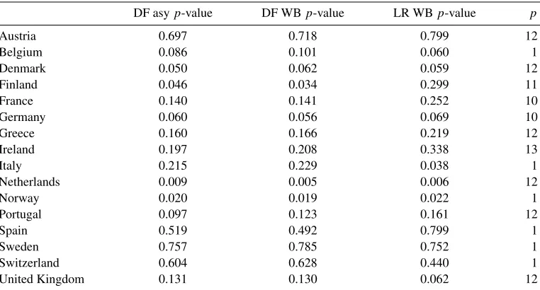
Table 1. Asymptotic and wild bootstrapp-values of DF and adaptive LR test.
DF asyp-value DF WBp-value LR WBp-value p
Austria 0.697 0.718 0.799 12
Belgium 0.086 0.101 0.060 1
Denmark 0.050 0.062 0.059 12
Finland 0.046 0.034 0.299 11
France 0.140 0.141 0.252 10
Germany 0.060 0.056 0.069 10
Greece 0.160 0.166 0.219 12
Ireland 0.197 0.208 0.338 13
Italy 0.215 0.229 0.038 1
Netherlands 0.009 0.005 0.006 12
Norway 0.020 0.019 0.022 1
Portugal 0.097 0.123 0.161 12
Spain 0.519 0.492 0.799 1
Sweden 0.757 0.785 0.752 1
Switzerland 0.604 0.628 0.440 1
United Kingdom 0.131 0.130 0.062 12
Note:The table reports asymptotic and wild bootstrapp-values for the DF–GLSμ, and wild bootstrapp-values for the
[image:17.485.51.432.379.584.2]the adaptive LR test leads to a clear rejection, with ap-value of around 4%. To a lesser extent, similar conclusions apply to Belgium and the UK. In summary, the example illustrates that the use of the more powerful adaptive LR test can indeed provide stronger evidence for the PPP hypothesis than using conventional tests, which confirms its useful role in the empirical analysis of macro-economic data.
8. DISCUSSION
In this paper, we have demonstrated that substantial power differences of unit root tests can arise in models with non-stationary volatility. We have shown that it is possible to construct a class of tests that have asymptotic power close to the envelope. The tests are based on non-parametric volatility estimation, and therefore do not require very specific assumptions on the parametric form of the volatility process. This approach can be extended in various directions.
First, for uniform consistency of the non-parametric volatility estimator, the volatility process needs to have continuous sample paths. This means that sudden level shifts are excluded. In practice, one might argue that these can be approximated arbitrarily well by smooth transition functions; furthermore, as shown by Xu and Phillips (2008), adaptive testing might be possible even in the presence of a finite number of discontinuities. The Monte Carlo experiment in this paper suggests that the procedure might perform quite well for level shifts in the volatility.
Secondly, the analysis is based on a deterministic volatility sequence. The asymptotic theory and the bootstrap method could be extended to allow for an exogenous volatility process, as long as it is independent of the Brownian motion defined from the standardized innovations. Hence, this excludes non-stationary volatility processes with statistical leverage effects, which are relevant in applications to equity prices. Note that our approach does not allow for stationary (GARCH-type) conditional heteroscedasticity, with or without leverage effects. It would be of interest to extend the analysis in this direction, leading to further possibilities for higher power.
The analysis in this paper can be extended to the multivariate case. The non-parametric volatility estimator has a very obvious extension to an estimator of a time-varying variance matrix; as long as the same kernel and window width is used for all variances and covariances, the resulting estimator will be positive semi-definite by construction. This can be used to construct more efficient cointegration tests or adaptive estimators of cointegrating vectors in the presence of non-stationary volatility. We are currently exploring this possibility; see Boswijk and Zu (2016).
ACKNOWLEDGEMENTS
We would like to thank the Co-Editor, Michael Jansson, and an anonymous referee for helpful comments and suggestions. Comments on earlier versions from Rob Taylor, Oliver Linton, Peter Phillips, Anders Rahbek, Ulrich M¨uller and Barbara Rossi are also gratefully acknowledged.
REFERENCES
Beare, B. K. (2016). Unit root testing with unstable volatility. Working paper, University of California, San Diego. Available at http://econweb.ucsd.edu/bbeare/pdfs/unitroot.pdf.
Boswijk, H. P. (2001). Testing for a unit root with near-integrated volatility. Tinbergen Institute Discussion Paper 01-077/4. Available at http://papers.tinbergen.nl/01077.pdf.
Boswijk, H. P. (2005). Adaptive testing for a unit root with nonstationary volatility. UvA-Econometrics Discussion Paper 2005/07. Available at http://dare.uva.nl/document/228023.
Boswijk, H. P. and Y. Zu (2016). Adaptive testing for cointegration with nonstationary volatility. Working paper, University of Amsterdam.
Cavaliere, G. (2004). Unit root tests under time-varying variances.Econometric Reviews 23, 259–92. Cavaliere, G. and A. M. R. Taylor (2007). Time-transformed unit root tests for models with non-stationary
volatility.Journal of Time Series Analysis 29, 300–30.
Cavaliere, G. and A. M. R. Taylor (2008). Bootstrap unit root tests for time series with non-stationary volatility.Econometric Theory 24, 43–71.
Doornik, J. A. (2013).An Object-oriented Matrix Programming Language – Ox 7. London: Timberlake Consultants Ltd (http://www.doornik.com).
Elliott, G., T. J. Rothenberg and J. H. Stock (1996). Efficient tests for an autoregressive unit root. Econometrica 64, 813–36.
Froot, K. A. and K. Rogoff (1995). Perspectives on PPP and long-run real exchange rates. In G. M. Grossman and K. Rogoff (Eds.), Handbook of International Economics, Volume 3, 1647–1688. Amsterdam: North-Holland.
Gin´e, E. and J. Zinn (1990). Bootstrapping general empirical measures.Annals of Probability 18, 851–69. Hansen, B. E. (1992). Convergence to stochastic integrals for dependent heterogeneous processes.
Econometric Theory 8, 489–500.
Hansen, B. E. (1995). Regression with nonstationary volatility.Econometrica 63, 1113–32.
Jansson, M. and M. Ø. Nielsen (2012). Nearly efficient likelihood ratio tests of the unit root hypothesis. Econometrica 80, 2321–32.
Jeganathan, P. (1995). Some aspects of asymptotic theory with applications to time series models. Econometric Theory 11, 818–87.
Kim, T.-H., S. Leybourne and P. Newbold (2002). Unit root tests with a break in innovation variance. Journal of Econometrics 109, 365–87.
Kim, K. and P. Schmidt (1993). Unit root tests with conditional heteroskedasticity.Journal of Econometrics 59, 287–300.
Le Cam, L. and G. L. Yang (1990). Asymptotics in Statistics: Some Basic Concepts. New York, NY: Springer.
Ling, S. and W. K. Li (1998). Limiting distributions of maximum likelihood estimators for unstable autoregressive moving-average time series with general autoregressive heteroscedastic errors. Annals of Statistics 26, 84–125.
Ling, S., W. K. Li and M. McAleer (2003). Estimation and testing for unit root processes with GARCH(1,1) errors: theory and Monte Carlo evidence.Econometric Reviews 22, 179–202.
Liu, R. Y. (1988). Bootstrap procedures under some non i.i.d. models.Annals of Statistics 16, 1696–708. Mammen, E. (1993). Bootstrap and wild bootstrap for high dimensional linear models.Annals of Statistics
21, 255–85.
Patilea, V. and H. Ra¨ıssi (2012). Adaptive estimation of vector autoregressive models with time-varying variance: Application to testing linear causality in mean.Journal of Statistical Planning and Inference 142, 2891–912.
Seo, B. (1999). Distribution theory for unit root tests with conditional heteroskedasticity. Journal of Econometrics 91, 113–44.
Taylor, M.P., D. A. Peel and L. Sarno (2001). Nonlinear mean-reversion in real exchange rates: toward a solution to the purchasing power parity puzzles.International Economic Review 42, 1015–42.
Van der Vaart, A. W. (1998).Asymptotic Statistics. Cambridge: Cambridge University Press. Wasserman, L. (2006).All of Nonparametric Statistics. New York, NY: Springer.
Xu, K.-L. and P. C. B. Phillips (2008). Adaptive estimation of autoregressive models with time-varying variances.Journal of Econometrics 142, 265–80.
APPENDIX A: PROOFS OF RESULTS
Proof of Lemma 2.1: Letαn=1+θn, and note thatXt =αnXt−1+σtzt, such thatXt= t−1
i=0α
i nσt−izt−i
(asX0=0) and hence
n−1/2Xun=fn(u)
u
0
gn(s)dWn(s), (A.1)
wherefn(u)=αnunandgn(u)=α−n un−1σn(u). It follows thatfn(u)=(1+c/n)un→ecu, andgn(u)→
e−cuσ(u), both inD[0,1]. The required result
n−1/2Xun→d
s
0
ec(u−s)σ(s)dW(s)
then follows from the continuous mapping theorem (as the integrand is non-stochastic).
The stochastic differential equation forXc(u) follows from the fact thatYc(u)=e−cuXc(u) satisfies
dYc(u)=e−cuσ(u)dW(u), and applying Itˆo’s lemma toXc(u)=ecuYc(u)=f(u, Yc(u)), leading to
dXc(u)=cecuYc(u)du+ecudYc(u)=cXc(u)du+σ(u)dW(u). (A.2)
Proof of Theorem 3.1: WriteJnas
Jn=
1 n2
n
t=1
σ−2
t X
2
t−1=
1
0
σn(u)−2Xn(u)2du,
where Xn(u)=n−1/2Xun. Lemma 2.1, Assumption 2.1 (including strict positivity of σ(·)) and the
continuous mapping theorem together imply
Jn d
→Jc=
1
0
σ(u)−2Xc(u)2du=
1
0
Zc(u)2du.
ForSn, we have
Sn−cJn=
1 n
n
t=1
σt−1Xt−1zt=
1
0
σn(u)−1Xn(u)dWn(u).
Using (σn(·), Xn(·), Wn(·)) d
→(σ(·), Xc(·), W(·)), andE[z2t]=1, it follows from Theorem 2.1 of Hansen
(1992) that
Sn d
→
1
0
σ(u)−1
Xc(u)dW(u)+cJc=
1
0
Zc(u)dW(u)+cJc.
Proof of Lemma 4.1: The proof is adapted from Hansen (1995), Theorem 2.1. We first show the result: max
1≤t≤nσ
2
t −σ
2
t p
→0. (A.3)
Let
wj N=
N
j=−N
k
j N
1{1≤t−j≤n}
−1 k j N
1{1≤t−j≤n},
such thatσ2
t =
N
j=−Nwj Nε
2
t−j, with N
j=−Nwj N=1. We have σt2−σ
2
t =R
a t +σ
2
tR b
t +R
c t +R
d
t, (A.4)
where
Rat =
N
j=−N
wj N(σt2−j−σ
2
t), R
b
t =
N
j=−N
wj N(z2t−j−1),
Rtc= N
j=−N
wj N(σt2−j−σ
2
t)(z
2
t−j−1), R
d
t =
N
j=−N
wj N(ε2t−j−ε
2
t−j).
Hansen’s proof that max1≤t≤n|Rta| p
→0, max1≤t≤n|σt2Rtb| p
→0 and max1≤t≤n|Rct| p
→0 can be directly extended to the present case. For the fourth term, we note thatεt =εt+(c/n)Xt−1. Therefore,
N
j=−N
wj N(εt2−j−ε
2
t−j)
≤2|c|1 n
N
j=−N
wj Nεt−jXt−1−j
+c2
n12
N
j=−N
wj NX2t−1−j
. (A.5)
Whenc=0, the right-hand side is identically zero; whenc=0, analogous to Hansen (1995), p. 1130, it follows that
max
1≤t≤n 1n
N
j=−N
wj Nεt−jXt−1−j
p
→0, (A.6)
max
1≤t≤n
1
n2
N
j=−N
wj NX2t−1−j =Op
N2
n2
p
→0, (A.7)
such that max1≤t≤nRtd p
→0. This proves (A.3).
Next, (A.3) can be strengthened to uniform consistency ofσn(·)2as follows. Assumption 2.1 implies
that supu∈[0,1]|σn(u)2−σ(u)2| →0 asn→ ∞, whereσn(u)=σun+1foru∈[0,1) andσn(1)=σn. This
definition implies thatσn(u)2−σn(u)2=σt2−σ
2
t foru∈[(t−1)/n, t /n). This in turn implies that
sup
u∈[0,1]
σn(u)2−σ(u)2 ≤ sup u∈[0,1]
σn(u)2−σn(u)2+ sup u∈[0,1]
σn(u)2−σ(u)2
= max
1≤t≤nσ
2
t −σ
2
t+ sup
u∈[0,1]
σn(u)2−σ(u)2
p
→0.
Proof of Theorem 4.1: Consistency ofJnfollows directly from Lemma 2.1 and 4.1 and the continuous
mapping theorem. ForSn, we use Sn−cJn=
1 n
n
t=1
σ−2
t Xt−1σtzt =
1
0
σn(u)−2σn(u)dUn(u),
where
Un(u) :=n−1/2
un
t=1
Xt−1zt =
u
0
Xn(s)dWn(s).
Because (Xn(·), Wn(·)) d
→(Xc(·), W(·)), andE[z2t]=1, it follows from Theorem 2.1 of Hansen (1992)
thatUn(u) d
→U(u) :=0uXc(s)dW(s). Combining this with Lemma 4.1, and the fact thatσ(·) is strictly
positive and non-stochastic, we find
Sn d
→
1
0
σ(u)−1dU(u)+cJ
c=
1
0
Zc(u)dW(u)+cJc=Sc.
Proof of Theorem 4.2: DefineXn∗(u)=n−1/2X∗ unand
Wn∗(u)=n−1/2
un
t=1
X∗t
σt
.
We prove the following joint convergence:
⎛ ⎜ ⎝
X∗n(u)
Wn∗(u)
σn(u) ⎞ ⎟ ⎠→d p
⎛ ⎜ ⎝
X0(u)
W(u) σ(u)
⎞ ⎟
⎠, (A.8)
withX0(u)=
u
0 σ(s)dW(s). Using the continuous mapping theorem, it then follows that
Jn∗=
1
0
σn(u)−2X∗n(u)
2
du→d p
1
0
σ(u)−2X0(u)2du=
1
0
Z0(u)2du=J0, (A.9)
and analogously to the proof of Theorem 4.1,
Sn∗=
1
0
σn(u)−1X∗n(u)dWn∗(u) d
→p
1
0
Z0(u)dW(u),
jointly with (A.9). This will prove the theorem, noting that the result forLR∗n=(Jn∗)−1/2S∗
nfollows easily
from the continuous mapping theorem.
To prove (A.8) for the wild bootstrap, note that
X∗n(u)
Wn∗(u)
=n−1/2
un
t=1
htz∗t, ht=
εt εt/σt
. (A.10)
Because{z∗t}t≥1 is i.i.d.N(0,1), independent of the data, it follows that conditionally on the data, this is
a bivariate Gaussian process with covariance kernelCn(u, s)=Vn(u∧s), whereVn(u) :=n−1
un
t=1 htht.
Definingh(s)=(σ(s),1), we prove that
Vn(u) p
→
u
0
uniformly inu∈[0,1]. This will imply
Xn∗(u)
Wn∗(u)
d
→p
X0(u)
W(u)
,
because the right-hand side is a Gaussian process with covariance kernelC(u, s)=V(u∧s). The joint convergence (A.8) then holds trivially, because of Lemma 4.1 and because conditionally on the data,σn(u)
has a degenerate distribution.
To prove (A.11), we start with the first diagonal elementV11,n(u) ofVn(u):
V11,n(u)=
1 n
un
t=1 ε2t =
1 n
un
t=1
ε2t +
c2
n3 un
t=1
X2t−1+2
c n2
un
t=1
εtXt−1.
For the first term,
1 n
un
t=1
εt2= 1 n
un
t=1
σt2z2t →p
u
0
σ2(s)ds=V11(u),
uniformly inu∈[0,1], which is (a special case of) the classical uniform convergence in probability result for the quadratic variation of a semimartingale. The second and third terms are both 0 underH0:θ=0;
underHn:θn=c/n, they are bothOp(n−1)=op(1), as
n−2
un
t=1
Xt2−1, n−1
un
t=1
εtXt−1
d
→ u
0
Xc(s)2ds,
u
0
Xc(s)σ(s)dW(s)
by the continuous mapping theorem and weak convergence to the stochastic integral, respectively. Next,
V22,n(u)=
1 n
un
t=1
ε2 t σ2 t = u 0
σn(s)−2dV11,n(s) p
→
u
0
σ(s)−2dV11(s)=u=V22(u),
by the continuous mapping theorem. Analogously,
V12,n(u)=n−1
un
t=1
ε2
t/σt p
→
u
0
σ(s)ds=V12(u).
This proves (A.11) and hence (A.8), and hence the theorem.
An analogous result obtains for the volatility bootstrap, based onεt∗=σtz∗t. In this case,htin (A.10) is
replaced byht=(σt,1), so that Lemma 4.1 directly implies (A.11).
Proof of Theorem 5.1: Consider, first, the case of a constant mean,dt =1. Becaused1=1 anddt =0
fort=2, . . . , n, it follows that underHn,
μ( ¯c)=
1 σ2 1
+ c¯2 n2 n t=2 1 σ2 t −1 Y1 σ2 1
− c¯ n
n
t=2
Yt−( ¯c/n)Yt−1
σ2
t
=Y1+Op(n−1/2),
and henceXd
t( ¯c)=Yt−Y1+Op(n−1/2)=Xt−X1+Op(n−1/2). From this, and the proof of Theorem 3.1,
it easily follows that
Sd n( ¯c)
Jd n( ¯c)
![Figure 1. Realization of volatility processes σ1–σ4. [Colour figure can be viewed atwileyonlinelibrary.com]](https://thumb-us.123doks.com/thumbv2/123dok_us/8553578.363546/7.485.70.410.366.595/figure-realization-volatility-processes-colour-gure-viewed-atwileyonlinelibrary.webp)
![Figure 2. Asymptotic power envelope and power curves for σ1–σ4. [Colour figure can be viewed atwileyonlinelibrary.com]](https://thumb-us.123doks.com/thumbv2/123dok_us/8553578.363546/8.485.82.408.69.291/figure-asymptotic-envelope-curves-colour-gure-viewed-atwileyonlinelibrary.webp)
![Figure 3. Log-real effective echange rates for 16 EU countries, 1973:1–2015:12. [Colour figure can beviewed at wileyonlinelibrary.com]](https://thumb-us.123doks.com/thumbv2/123dok_us/8553578.363546/16.485.60.425.67.308/figure-effective-echange-countries-colour-gure-beviewed-wileyonlinelibrary.webp)