Testing for Quaternion Propriety
P. Ginzberg and A. T. Walden,
Senior Member, IEEE
Copyright (c) 2011 IEEE. Personal use of this material is permitted. However, permission to use this material for any other purposes must be obtained from the IEEE by sending a request to [email protected]. Paul Ginzberg and Andrew Walden are both at the Department of Mathematics, Imperial College London, 180 Queen’s Gate, London SW7 2BZ, UK. (e-mail: [email protected] and [email protected])
Abstract
We consider the problem of testing whether a quaternion-valued Gaussian random vector is proper. The quaternion covariance matrix fully describes the second order properties of a quaternion random vector only if the distribution is proper. The exact distribution of the likelihood ratio test under the hypothesis of propriety is derived for general sample size,N, and vector dimensionality, p.As this is in
terms of Meijer’s G-function, various approximations are considered, including Box-type and saddlepoint approximations. We find in particular that a new approach matching the first three cumulants is easy to implement and extremely accurate.
Keywords
quaternion random vector, structured covariance, likelihood ratio test, improperness, Meijer’s G-function
I. Introduction
Recently there has been much interest in quaternion-valued signal processing [5], [10], [15], [16], [17], [20], [22], [23], [24], [28]. Many multivariate problems based on vector sensors may be readily modeled in the quaternion domain which accounts naturally for the correlated nature of the signal components. Applications of quaternion signal processing include multicomponent seismic velocity analysis [5], singular value decomposition for vector sensing [10], sequential best rotation [15] for polarized source separation in convolutive mixture models, multiple signal classification (MUSIC) spectrum estimation [17], block coding [20], [32], and adaptive filtering [22].
As is the case with complex-valued random vectors, the quaternion covariance only fully cap-tures the second order properties of proper quaternion random vectors. In the more general improper case, further information is contained in three complementary covariance matrices. It is shown in [28], [29] that using quaternion linear processing for partial least squares, principal component analysis, multivariate linear regression or canonical correlation analysis is subopti-mal for improper quaternion random vectors. For the same reason the quaternion widely linear adaptive filter is introduced in [23] and incorporated into their quaternion least mean square algorithm, allowing for a unified approach to adaptive filtering of both proper and improper quaternion signals.
It is hence timely to consider the problem of testing whether a quaternion-valued Gaussian random vector is proper. [27] studies the likelihood ratio test (LRT) from a geometric and
information-theoretic perspective. We will instead consider structured real covariance matrices and concentrate on the exact distribution of the test statistic and its accurate approximation.
In the remainder of this Introduction we define mathematically the problem we wish to solve. In Section II we firstly provide some basic definitions and introduce notation, along with the augmented covariance matrix. Following [28] we define propriety for quaternions. In Section III the testing problem is developed in terms of two nested hypotheses. The LRT statistic and its moments follow. The Box-type parameters are identified. The asymptotic and exact distributions of the statistic are derived in Section III, the latter involving Meijer’s G-functions. As this is inconvenient in practice, Section V examines various approximations, including Box-type and saddlepoint approximations. Section V-C introduces a new approach matching the first three cumulants which is easy to implement and extremely accurate. Section VI considers asymptotic robustness to nonGaussianity. Section VII provides our concluding comments.
A. The problem
Leta,b,c,dbe real-valuedp-dimensional jointly Gaussian random variables (column vectors). Then q = a+bi +cj +dk follows a (possibly improper) p-dimensional quaternion Gaussian distribution. Here 1,i,j,k are the 4 basis elements of the quaternions (see Section II-A). Studying the distribution ofqis equivalent to studying the distribution of the 4p-dimensional real Gaussian random variable r= [aT,bT,cT,dT]T with covariance matrix⌃
r =E{rrT}. We are assuming
throughout thatE{r}=0, but this can be relaxed by subtracting the sample mean and replacing
N by N 1 in all results.
In this paper we consider the hypothesis test H0 : the 4p⇥4p covariance matrix ⌃r from a
real-valued multivariate Gaussian distribution has quaternion structure, defined in (8), against the default alternativeH1:⌃r does not have quaternion structure.
Just as in the complex-valued case, where testing that an appropriate 2p⇥2pcovariance matrix
has complex structure, defined in (10), is equivalent to testing for propriety for p-dimensional complex-valued Gaussian vectors [30], so testing that the 4p⇥4p covariance matrix ⌃r has
quaternion structure is equivalent to testing for propriety for p-dimensional quaternion-valued Gaussian vectorsq.
II. Background
A. Basics
The quaternions Hare a 4-dimensional real division algebra. We denote the 4 basis elements by 1,i,j,k. In this basis, a quaternion can be written asq =a+bi +cj +dk with a, b, c, d2R. i,j,k satisfy i2 = j2 = k2 = ijk = 1, ij = ji = k, jk = kj = i, ki = ik = j and quaternion multiplication is associative, distributive but not commutative.
The conjugate of q isq⇤ =a bi cj dk. The quaternion norm is defined as|q|=pqq⇤ =
[a2+b2+c2+d2]1/2. i
0 is a pure unit quaternion i↵|i0|= 1 and its real part is zero. The inverse of a quaternion q 6= 0 is q 1 = q⇤/|q|2. For a quaternion matrix Q we denote the conjugate transpose by QH = (Q⇤)T.The product of two matrices Q2Hm⇥n and S 2Hn⇥p is P =QS with (i, j)th elementp
i,j =Pn`=1qi,`s`,j.
B. Covariance matrices
Analogously to improper complex random variables, the second-order properties of q, given by the 4p⇥4preal covariance matrix
⌃r=E{rrT}= 2 6 6 6 6 6 6 4 ⌃a ⌃a,b ⌃a,c ⌃a,d ⌃b,a ⌃b ⌃b,c ⌃b,d ⌃c,a ⌃c,b ⌃c ⌃c,d ⌃d,a ⌃d,b ⌃d,c ⌃d 3 7 7 7 7 7 7 5 , (1)
(⌃a,b = E{abT} and ⌃a = E{aaT}), are not fully specified by its (quaternion) covariance
matrix⌃q=E{qqH}.
Given a quaternion q0 and a pure unit quaternion i0 define the involution q0(i0) = i0q0i01 = i0q0i0.
Note that i,j and k are all pure unit quaternions. We define an augmented quaternion vector as q=Ar= 2 6 6 6 6 6 6 4 q q(i) q(j) q(k) 3 7 7 7 7 7 7 5 = 2 6 6 6 6 6 6 4 q iqi jqj kqk 3 7 7 7 7 7 7 5 = 2 6 6 6 6 6 6 4 a+bi +cj +dk a+bi cj dk a bi +cj dk a bi cj +dk 3 7 7 7 7 7 7 5 , (2)
where (e.g., [24]) A= 2 6 6 6 6 6 6 4 Ip iIp jIp kIp Ip iIp jIp kIp Ip iIp jIp kIp Ip iIp jIp kIp 3 7 7 7 7 7 7 5 . (3)
It is worth noting that if c = d = 0, so that the quaternion vector is just a complex vector, then [aT,bT]T can be taken to the augmented complex vector [(a+bi)T,(a bi)T]T using the well-known submatrix of A[21, p. 31]: 2 4 Ip iIp Ip iIp 3 5. (4)
The second-order properties ofq are fully specified by its augmented covariance matrix
⌃q =E{q qH}=A⌃rAH. (5)
Indeed, since A 1 = 14AH we can easily recover the real covariance matrix:
⌃r= 161 AH⌃qA. (6)
Expanding (5) inp⇥p blocks gives [28, p. 3505]
⌃q = 2 6 6 6 6 6 6 4 ⌃q ⌃q,q(i) ⌃q,q(j) ⌃q,q(k) ⌃(i) q,q(i) ⌃ (i) q ⌃(i)q,q(k) ⌃ (i) q,q(j) ⌃(j) q,q(j) ⌃ (j) q,q(k) ⌃ (j) q ⌃(j)q,q(i) ⌃(k) q,q(k) ⌃ (k) q,q(j) ⌃ (k) q,q(i) ⌃ (k) q 3 7 7 7 7 7 7 5 (7)
where terms of the form⌃(i)
q,q(k) denote involutions, e.g.,⌃
(i)
q,q(k) = i⌃q,q(k)i.Since all the blocks
in ⌃q can be derived from the first row of blocks, the second-order properties of q can be
described by specifying the covariance⌃q along with three complementary covariance matrices
⌃q,q(i) = E{qiqHi}
⌃q,q(j) = E{qjqHj}
C. Propriety
We now give the definitions of propriety following [28].
Definition 1: q is H-proper, (or just proper), i↵⌃q,q(i) = 0,⌃q,q(j) = 0 and ⌃q,q(k) = 0.
Definition 2: q is Cj-proper i↵ ⌃
q,q(i)=0 and⌃q,q(k)=0.
Proposition 1: q is H-proper (proper) i↵
⌃r = 2 6 6 6 6 6 6 4 ⌃a ⌃b,a ⌃c,a ⌃d,a ⌃b,a ⌃a ⌃d,a ⌃c,a ⌃c,a ⌃d,a ⌃a ⌃b,a ⌃d,a ⌃c,a ⌃b,a ⌃a 3 7 7 7 7 7 7 5 . (8) q isCj-proper i↵ ⌃r = 2 6 6 6 6 6 6 4 ⌃a ⌃a,b ⌃c,a ⌃c,b ⌃b,a ⌃b ⌃d,a ⌃d,b ⌃c,a ⌃c,b ⌃a ⌃a,b ⌃d,a ⌃d,b ⌃b,a ⌃b 3 7 7 7 7 7 7 5 (9) = 2
4 ⌃Re(z) ⌃Im(z),Re(z)
⌃Im(z),Re(z) ⌃Re(z)
3
5=...⌃r,say, (10)
wherez =⇥aT,bT⇤T +⇥cT,dT⇤Tj.
Proof: These follow from (6) and (7). More easily, the form of (8) is immediate from [28, lemma 8] while (9) is readily derived from [28, Table 1].
Quaternion propriety can be interpreted geometrically as invariance of the second-order prop-erties under the transformations (rotations) of the form q 7! qu where u is a unit quaternion [28, lemma 9]. Invariance under q 7! uq gives a di↵erent ‘handedness’ of quaternion propriety [26]. Studying either type of handedness is however equivalent, since taking conjugates switches the handedness ofq.
Algebraically, propriety is preserved by quaternion linear transformationsq7!Lq,L2Hm⇥p [28, Lemma 1]. Thus, the hypothesis test H0 v.s. H1 is invariant under q 7! Lqu where L 2 Hp⇥p is invertible and u is a unit quaternion. In particular, propriety is preserved by all rotationsq7!uqv,|u|=|v|= 1.
Cj-propriety ofq is equivalent to the complex propriety ofz or the joint complex propriety of a+cj andb+dj [28, p. 3507].
Note that if q is H-proper then ⌃q = 4⌃a+ 4⌃b,ai + 4⌃c,aj + 4⌃d,ak and if z is complex
proper then ⌃z= 2⌃Re(z)+ 2⌃Im(z),Re(z)j.
Finally, in the scalar case (p= 1) propriety ofqis equivalent to sphericity ofr, i.e.,qis proper i↵a,b,c,dare independent and identically distributed (IID). A LRT for propriety then reduces to Mauchly’s test [14].
III. Testing for Quaternion structure
A. Covariance structures
Here we will link the real-valued covariance matrices in (8) and (9) to the work of [1].
Definition 3: Let PR denote the set of 4p ⇥4p symmetric positive definite matrices. Let
PC ⇢ PR and PH ⇢ PR denote the set of symmetric positive definite matrices of the form (9) (or (10)), and (8), respectively. In the terminology of [1, pp. 394, 403–404], PC is the set of covariance matrices with complex structure and PH is the set of covariance matrices with quaternion structure. Clearly PH ⇢PC.
Consider our hypothesis test stated in Section I-A. Because the quaternion structure is a special case of complex structure, we can exploit the nested nature of the implied models to build a direct test from two of the tests discussed in [1]. Consider two hypothesis tests with default alternatives and null hypotheses as follows:
1. Test 1. H0C: the 4p ⇥4p covariance matrix ⌃r from a real-valued multivariate Gaussian
distribution has complex structure. [HC
0: ⌃r 2PCversus H1C: ⌃r2PR\PC.]
2. Test 2. H0H: the 4p ⇥4p covariance matrix ⌃r with complex structure (⌃r =
... ⌃r) has
quaternion structure. [HH
0: ⌃r2PH versusH1H: ⌃r 2PC\PH.] Since PH ⇢PC,we know H0H is nested within H0C.
Now letq1, . . . ,qN be an IID sample of quaternion Gaussian random variables from the distri-bution ofqand letr1, . . . ,rN be the corresponding 4p-dimensional real-valued random variables, withN 4p,from a Gaussian distribution with mean vector zero and positive-definite and sym-metric covariance matrix ⌃r. We shall denote the maximum likelihood estimator of⌃r by ˆ⌃R,
where ˆ ⌃R= 1 N N X `=1 r`rT`. (11)
Lemma 1: Consider⌃r 2PR,defined as in (1). This can be expressed as
⌃r = 2
4 ⌃Re(z) ⌃Re(z),Im(z)
⌃Im(z),Re(z) ⌃Im(z)
3 5. Define J1 = 2 402p I2p I2p 02p 3 5. (12)
Let ˆc:PR!PC be a projection such that ˆc(2⌃r) = 2
4 ⌃Re(z)+⌃Im(z) ⌃Re(z),Im(z) ⌃Im(z),Re(z)
⌃Im(z),Re(z) ⌃Re(z),Im(z) ⌃Re(z)+⌃Im(z)
3 5
=⌃r+J1⌃rJ1T. (13)
Then ˆ⌃C= ˆc( ˆ⌃R) is the maximum likelihood estimator of ⌃r underH0C.
Proof: We wish to maximise the likelihood function (2⇡) 2pNdet{⌃ C} N/2exp ⇣ trn⌃ 1 C ⌃ˆR o /2⌘ (14)
over⌃C2PC. In consideration we introduce Lemma 2.
Lemma 2: For ⌃C2PC, trn⌃C1⌃ˆCo= trn⌃C1⌃ˆRo.
Proof: This is given in Appendix–A. By Lemma 2, (14) is equal to (2⇡) 2pNdet{⌃ C} N/2exp ⇣ trn⌃ 1 C ⌃ˆC o /2⌘.
From the classical case, this is maximised over⌃C2PR PC by setting⌃C= ˆ⌃C. (See also [1, eqn. 12, Th. 1].) This completes the proof of Lemma 1.
Lemma 3: Consider...⌃r 2PC,defined as in (10) and define
J2 = 2 6 6 6 6 6 6 4 0p 0p 0p Ip 0p 0p Ip 0p 0p Ip 0p 0p Ip 0p 0p 0p, 3 7 7 7 7 7 7 5 . (15)
Let ˆh:PC!PH be a projection such that ˆh(2...⌃r) = 2 6 6 6 6 6 6 4 ⌃a+⌃b ⌃a,b ⌃b,a ⌃d,b ⌃c,a ⌃c,b ⌃d,a ⌃b,a ⌃a,b ⌃a+⌃b ⌃c,b ⌃d,a ⌃c,a ⌃d,b ⌃c,a ⌃d,b ⌃c,b+⌃d,a ⌃a+⌃b ⌃a,b ⌃b,a ⌃c,b+⌃d,a ⌃d,b ⌃c,a ⌃b,a ⌃a,b ⌃a+⌃b 3 7 7 7 7 7 7 5 =...⌃r+J2 ... ⌃rJ2T. (16)
Then ˆ⌃H = ˆh( ˆ⌃C) = ˆh(ˆc( ˆ⌃R)) is the maximum likelihood estimator of ⌃r underH0H.
Proof: We wish to maximise the likelihood function (2⇡) 2pNdet{⌃ H} N/2exp ⇣ trn⌃ 1 H ⌃ˆR o /2⌘ (17)
over⌃H2PH. In consideration we introduce Lemma 4.
Lemma 4: For ⌃H 2PH, trn⌃H1⌃ˆHo= trn⌃H1⌃ˆRo.
Proof: This is given in Appendix–A. By Lemma 4, (17) is equal to (2⇡) 2pNdet{⌃ H} N/2exp ⇣ trn⌃ 1 H ⌃ˆH o /2⌘.
This is maximised over⌃H2PR PH by setting ⌃H = ˆ⌃H. (See also [1, eqn. 56, Th. 3].) This completes the proof of Lemma 3.
B. Nature of the Test
LetTCbe the LRT statistic for Test 1, andTH be the LRT statistic for Test 2. From [1, Th. 1] TCand ˆ⌃Care independent under H0C. Applying Test 2 to ˆ⌃C we obtain another LRT statistic TH which is a function of ˆ⌃Cand hence is independent ofTC. The LRT statistic for testing H0H versusH1C takes the simple form T =TC·TH.
Proposition 2: The likelihood ratio (LR) for testing H0H versus H1H is given by TH= [det{⌃ˆC}/det{⌃ˆH}]N/2.
Proof: By Lemmas 1 & 3 the LR is
" det{⌃ˆC} det{⌃ˆH} #N/2 ·exp ⇣ trn⌃ˆ 1 H ⌃ˆR o /2⌘ exp⇣ trn⌃ˆ 1 C ⌃ˆR o /2⌘.
By Lemmas 4 & 2, trn⌃ˆ 1 H ⌃ˆR o = trn⌃ˆ 1 H ⌃ˆH o = tr{I4p} = trn⌃ˆC1⌃ˆC o = trn⌃ˆ 1 C ⌃ˆR o , so the exponentials cancel.
Proposition 3: The LR for testingH0C versusH1C is
TC= [det{⌃ˆR}/det{⌃ˆC}]N/2.
Proof: Proceeds as Proposition 2; see also [30, p. 828].
Consider H0, H1, defined in Section I-A. Since P( ˆ⌃R 2 PC) = 0, the maximum likelihood underH1C and underH1 are almost surely equal. Also, H0 =H0H. The LRT statistic for testing H0 versusH1 is therefore
T =TC·TH= [det{⌃ˆR}/det{⌃ˆH}]N/2. (18) T satisfies 0 T 1, since it is an LR and PH ⇢PR. We reject the null hypothesis for small values ofT.
Now let us consider the moments ofT.By independence we can obtain the momentsE{Th}=
E{Th
C}E{THh}.
Proposition 4: Under H0 the LRT statisticT forH0 versusH1 has moments E{Th}=K d3p 2 e Y j=1 [N(h+ 1) 4p+ 2j 1] N(h+ 1) + 2 j b j 1 3 c 2 , (19)
wherebxc is the integer part of x,dxeis the smallest integer greater or equal to x, andK does not depend on h.
Proof: This is given in Appendix–B.
We now identify a general class of distributions containing the LRT statistic T.
Definition 4: A random variable 0W 1 is said to be of Box-type [2] if, for allh2N, E{Wh}=K "Qk j=1y yj j Qm i=1xxii #h Qm i=1 [xi(1 +h) +⇠i] Qk j=1 [yj(1 +h) +⌘j] , (20)
where K = Qkj=1 (yj+⌘j)/Qmi=1 (xi+⇠i), so E{W0} = 1, and Pmi=1xi = Pkj=1yj, xi > 0, yj >0.
Comparing (19) and (20) we see that T is a random variable of Box-type with
xi =yj =N;m=k=d3p/2e; (21) ⇠i= 4p+ 2i 1;⌘j = [2 j b(j 1)/3c]/2, (22)
and K in (19) is K= d3p 2 e Y i=1 [N+⌘i] [N +⇠i] . (23)
Next, we will consider the non-negative random variable M = 2 logT. IV. Test Statistic and Its Distribution
A. Asymptotic Distribution
From Wilks’ theorem [33, p. 132] under H0,asN ! 1,
M = 2 logT !d 2f (24) i.e., M tends in distribution to 2
f. Here f denotes the degrees of freedom for the test and is given by [2, eqn. 73] f = 2 2 4 m X i=1 ⇠i k X j=1 ⌘j 12(m k) 3 5 = d3p/2Xe i=1 [8p+ 4 5i b(i 1)/3c] = 3p(2p+ 1). (25)
This is equal to the di↵erence between the number of free parameters in the covariance matrix underH1, namely 2p(4p+ 1),and underH0, namelyp(2p 1). The asymptotic distribution (24) is given in [27] (along with asymptotic distributions of other related likelihood ratio statistics).
B. Exact Distribution
We firstly show thatT can be written as a product of powers of independent Beta-distributed random variables.
Proposition 5: Assume W has moments given by (20) where m = k, xi = yi for all i and ⌘i > ⇠i > xi for all i(parameters can be reordered if necessary). ThenW ⇠Qmi=1Vixi, where Vi are independently distributed as Beta(⇠i+xi, ⌘i ⇠i) random variables.
Proof: Similarly to [13, p. 122], for allh2Csuch that Re(h)> ⇠i xi, E{Vxih
i }=
(xi+⌘i) (⇠i+xi(1 +h)) (xi+⇠i) (⌘i+xi(1 +h))
. (26)
Hence the moments match and so does the distribution which is bounded and hence uniquely determined by the moments.
Exact probability density functions (PDFs) of products of powers of independent Beta ran-dom variables are given as H-functions in [13, eq. (4.15)]. Furthermore, T1/N is a product of independent Beta random variables; the PDFs of such products are given as G-functions in [3, eq. (4.8)].
Definition 5: Fox’s H-function is defined by the following Mellin-Barnes integral [3]: Hq,ru,v 2 4z (a1, ↵1), . . . ,(ap, ↵q) (b1, 1), . . . ,(bq, r) 3 5= 1 2⇡i Z L Qu j=1 (bj js)Qvj=1 (1 aj+↵js) Qr j=u+1 (1 bj+ js)Qqj=v+1 (aj ↵js) zsds. (27) The path of integration L is chosen such that the poles (bj +n)/ j, j = 1, . . . , u, n 2 N are separated from the poles (aj 1 n)/↵j, j = 1, . . . , v, n2N. The parameters are 0v q, 0ur,↵i, j 2[0,1[, ai, bj 2C.
In all our uses, we will have v = 0 and the path of integration L will be a vertical line from i1 to + i1.
Definition 6: Meijer’sG-function is a special case of the H-function Gu,vq,r 2 4z a1, . . . , aq b1, . . . , br 3 5=Hq,ru,v 2 4z (a1,1), . . . ,(aq,1) (b1,1), . . . ,(br,1) 3 5. (28)
The moment generating function for M is given by M(s) =E{esM}=E{T 2s}so by Proposi-tion 5 M(s) =K d3p 2e Y j=1 [N(1 2s) +⇠j] [N(1 2s) +⌘j] (29) for Re( 2s)>maxi( ⇠i xi) = 4p 1 N,with⇠i, ⌘i, K given in (22) and (23).
Theorem 1: With parameter values as in (21) and (22), the PDF of M is given by fM(x) = Ke x/2 2N Gm,0m,m 2 4e x/(2N) ⌘1, . . . , ⌘m ⇠1, . . . , ⇠m 3 5, (30)
where the constant K is defined in (23). The cumulative distribution function (CDF) is FM(x) =Ke x/2Gm+1,0m+1,m+1 2 4e x/(2N) ⌘1, . . . , ⌘m,1 N ⇠1, . . . , ⇠m, N 3 5. (31)
Proof: This is given in Appendix–D.
To be useful, the G-function expressions for the PDF and CDF in (30) and (31), respectively, need to be computable quantities. We examined a number of symbolic computation engines which in theory have arbitrary-precision implementations of Meijer’sG-function, and encountered problems with each implementation. We were however able to compute exact quantiles of the distribution of M, using version 13 of MapleR, by adding an ad-hoc correction whenever (31)
erroneously evaluated to FM(x) 1. These exact quantiles are used to compare approximations in section V-H.
The cumulants of M can be easily obtained from the cumulant generating function log M(s). j = d jlog M(s) (ds)j s=0 =[ 2N]j d3p/2Xe i=1 h (j 1)(N +⇠i) (j 1)(N +⌘i)i, (32) where (x) = [d log (x)]/dx is the digamma function and its derivatives are polygamma func-tions (trigamma, tetragamma, . . .). 1 is the mean, 2 is the variance, 3/3/22 is the skewness and 4/22 is the excess kurtosis.
V. Approximating Distributions Using a 2
f distribution to approximate the distribution ofM as in (24) will generally give poor results for finite N.Routine computation of the exact distribution for hypothesis testing is not straightforward. We now consider approximation methods and their performance. We briefly outline various possible approaches which we will compare later by making use of the exact distribution. We firstly note that since the distribution ofT is of Box type, we may approximate the distribution ofM = 2 logT using methods in [2].
A. Bartlett adjustment
One such method introduces a Bartlett adjustment C,approximating M by the distribution of C 2f, where f = 3p(2p + 1) here, as in (25). C is chosen so that the cumulants of the approximation match those of M up to an error of order O N 2 . Box’s method [2, p. 338] implies the Bartlett adjustment CBox= (12N)/(12N+ 1 20p).
This approximation is convenient since it does not require the use of a computer. A more ac-curate approximation is obtained if one instead chooses the Bartlett adjustmentCexact=f 11,
which matches the mean of M exactly, but we will not examine this option further since it is superseded by the gamma approximation of the next section. An analysis is given in [18] where various choices of Bartlett adjustment for tests 1 and 2 are compared.
B. Gamma approximation
As suggested in [7], we can also approximate M by a Gamma random variable with PDF f(x) = ( r/ (r))xr 1exp( x), for x, r, > 0, with r = 21/2, = 1/2. Such a random variable has the same mean and variance as M. Scaled 2 distributions are special cases of the Gamma distribution where the first (shape) parameter is a half integer, so this approach corresponds to fitting both the scale and the degrees of freedom of a scaled 2 approximation.
C. A new F-approximation
Based on the Pearson system of curves [9], Box uses distributions of scaled F- and Beta-distributed random variables, bF(f1, f2) or bBeta (f1, f2), respectively, where the distribution and parameters are chosen so that the first four cumulants match those ofM up to an error of order O(N 3).
We suggest instead to match the first 3 cumulants exactly, leading to greatly increased accuracy. It does not appear this exact approach has been used before. We ran a numerical study of all combinations p10000, N 4p+ 2000 and concluded that cases requiring a Beta distribution
do not arise and that it will be possible to match the first 3 cumulants using anF distribution whenever N 4.13p+ 0.5, i.e., nearly always considering that N 4p is a requirement. The parameters are then given by
f1 = 41 212 22+13 /(4122 213+23);
f2 = (4212 822+ 613)/(13 222); (33) b = 21 212 22+13 /(2212 422+ 313).
D. Box’s 2 series
Following [2] we can expand the distribution function of M as FM(x) =KB n 1 X j=0 ajF 2 f+2j(⇢x) + O N n , (34)
whereKB=K(⇢N) f /2. Using the iterative scheme of [6], which is essentially a new utilization of the algorithm which computes moments from cumulants, the coefficients are given by
a0 = 1; aj = 1 j j X i=1 i!iaj i , j= 1, . . . , n 1; !i = ( 1) i+1 i(i+ 1)(⇢N)i ⇥ d3p 2e X `=1 [Bi+1((1 ⇢)N +⇠`) Bi+1((1 ⇢)N+⌘`)],
where Bi(x) denotes the Bernoulli polynomial of degreei. The free scaling parameter⇢is chosen so that a1 = 0. Using [4, eqn. 1.7],⇢= 1 [1/(f N)]Pd
3p
2e
`=1 [B2(⇠`) B2(⌘`)] =CBox1.
It is proven in [6] that for x < 4⇡N, the series (34) converges to FM(x) as n! 1, meaning
that an arbitrary precision (exact) value can be computed. For x 4⇡N, the series diverges if too many terms are taken, as is generally the case with asymptotic expansions, but this is unlikely to be a problem in practice.
This approximation is often applied with the parameter choicen= 3, and possibly a renormali-sation. Due to its poor performance, we have chosen insteadn= 5 in our numerical comparisons.
E. Lugannani & Rice saddlepoint approximation
Consider an exponentially tilted version of M,Ms say, i.e., fMs(x) = esxfM(x)/ M(s). Then
since Ms(t) = M(s+t)/ M(s) the cumulants ofMs are
¯ j(s) = d jlog Ms(t) (dt)j t=0 = ( 2N)j d3p/2Xe i=1 h (j 1)(N(1 2s) +⇠i) (j 1)(N(1 2s) +⌘ i) i .
LetFN(·) andfN(·) denote, respectively, the standard Gaussian CDF and PDF. The Lugannani & Rice saddlepoint approximation [12], truncated to two terms is
FM(x)⇡FN(˜x) +fN(˜x) x1˜ 1
s0¯1/22 (s0)
!
(35) where ˜x = sign(s0){2 [s0x log( M(s0))]}1/2 and s0 is the unique solution of ¯1(s) =x. Since the derivative of ¯1(s) is ¯2(s)>0,s0 can easily be found numerically, e.g., by Newton’s method.
The distribution of M is asymptotically 2f, not asymptotically normal and hence (35) does not converge toFM(x) asN ! 1. To solve this problem, we considered using the approximation of [31] which generalises the Lugannani & Rice saddlepoint approximation to non-normal basis distributions. However, using a Gamma basis distribution provided no significant improvement, except obviously for large N.
F. Jensen’s large deviation approximation
In [7], [8] Jensen applies the Gamma approximation to the exponentially tilted Ms, which yields the following approximation forM:
FM(x) ⇡ M(s0) ✓ 1 +s0¯2(s0) x ◆ x2/¯ 2(s0) ⇥ ✓ x2 ¯ 2(s0) , xs0+ x 2 ¯ 2(s0) ◆
where as previously s0 solves ¯1(s) = x, and (a, b) denotes the incomplete gamma function (a, b) =hRb
0 xa 1exp( x)dx
i
/ (a).
Whilst for all of the previously described approximations the relative error (36) tends to infinity if one takesx! 1, the relative error of this approximation instead goes to 0, making it particularly suitable for approximating the extreme tail.
G. Direct simulation
The moments (19), which fully determine the null distribution of T, and hence ofM, do not depend on the true covariance matrix⌃r.Hence we can assume⌃r=I4p when simulatingM. For each sample of size N the maximum likelihood estimator ˆ⌃R in (11) is computed. ˆ⌃H is then given by (13), (15) and (16), andT by (18).
H. Computational results
For a chosen combination of p and N we define the relative error of the approximation Fapprox(x) to FM(x) as
Fapprox(x) FM(x) min [FM(x),1 FM(x)]
, (36)
where FM(x) is given in (31) and Fapprox(x) is any of the approximate CDFs discussed in this Section. The e↵ect of the divisor is to make the error relate to the corresponding tail probability, depending on whether x corresponds to a value in the left or right tail. Since we will reject the
hypothesis of propriety when M is larger than some critical value, we will be most interested in the region around FM(x) = 0.95 and 0.99. In Fig. 1 the relative error is plotted againstx for our considered approximation methods for the case p = 4, N = 32. The various methods used have been given both plot symbols and labelled A-F in the legend of the figure according to the subsection where they are discussed, and we will use this labelling in what follows. The top axis shows the value ofFM(x) (as a percentage) corresponding toxon the bottom axis. We conclude that the new scaled F-approximation (method C), the saddlepoint approximation (method E) and the large deviation method (method F), perform best. Of these the scaledF-approximation is the easiest to implement in practice.
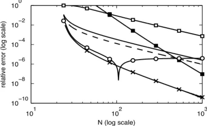
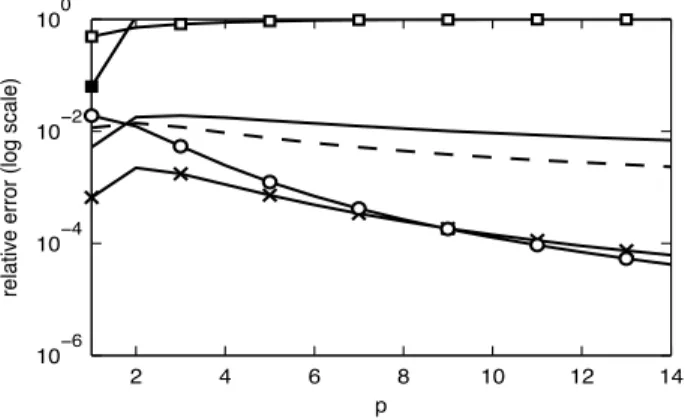
To see whether our conclusions are generally true for impropriety testing for a variety of p and N we firstly look at the relative error of approximation at the 95th percentile of FM(x). Fig. 2 shows this relative error for fixedp= 6 and increasing values ofN.We see that the errors for approximations A, B, C, D, E, and F, behave roughly like O (N r) with r = 2,2,3,5,0,2 respectively. Fig. 3 shows this relative error forp = 1, . . . ,14 andN = 5p. Finally, Fig. 4 gives the relative error for varying p and N = 16p. In all cases our earlier conclusions are borne out, particularly that the scaledF-approximation performs extremely well. Let x0 be the 99th percentile ofFM(x) and letFapprox(x) be one of the approximate CDFs of subsections A–G. The values given in Table I are then 100(1 Fapprox(x0))%,a quantity which is ideally 1%. For each p the entries start at the minimum N value of 4p and the other entries are for 5p,8p and 16p. The scaledF approximation (method C) requiresN 4.13p+ 0.5 so that it cannot be used for N = 4p and thus the corresponding entry is marked by ‘N/A.’ Again we see that methods C, E and F all perform very well. Table I also includes direct simulation results (method/subsection G) with the empirical CDF calculated from 100 000 independent simulations of M = 2 logT. Even with so many independent simulations the simulated results can be relatively inaccurate compared with the simple scaledF approximation.
VI. Asymptotic Robustness to NonGaussianity
As with the LRT for complex propriety [19], our LRT for quaternion propriety will be sensitive to departures from Gaussianity which could be an issue when applying the test to physical data.
We can write the hypothesis that⌃rhas quaternion structure in the form [⌃r h(ˆˆ c(⌃r))]/var{r1}= 04p. Taking f non-redundant equations from this, the LRT for quaternion structure satisfies the scaling condition for [25, Corollary 1] to hold. Consequently, if instead of being multivariate
method p N A B C D E F G 1 4 0.0398 0.7973 0.9806 5.2512 0.9961 1.0334 0.997 5 0.3126 0.9021 0.9972 1.5443 0.9790 1.0078 0.950 8 0.7688 0.9756 1.0000 1.0164 0.9893 0.9980 0.976 16 0.9535 0.9956 1.0000 1.0002 0.9991 0.9997 0.977 2 8 0.0002 0.6318 0.9812 40.612 0.9914 1.0646 1.048 10 0.1429 0.8876 0.9988 7.9486 0.9788 1.0086 1.009 16 0.6790 0.9791 0.9999 1.2280 0.9979 1.0021 1.004 32 0.9339 0.9965 1.0000 1.0029 0.9999 1.0004 0.995 4 16 0.0000 0.5115 N/A 96.174 0.9873 1.0930 0.978 20 0.0496 0.9219 0.9982 49.217 0.9952 1.0084 1.046 32 0.5607 0.9875 0.9999 4.1031 0.9998 1.0013 1.016 64 0.9034 0.9980 1.0000 1.0412 1.0000 1.0002 1.004 6 24 0.0000 0.4671 N/A 99.982 0.9849 1.1058 0.985 30 0.0167 0.9442 0.9987 89.100 0.9988 1.0059 0.966 48 0.4616 0.9914 0.9999 15.430 0.9999 1.0008 1.023 96 0.8737 0.9986 1.0000 1.2439 1.0000 1.0001 1.021 12 48 0.0000 0.4287 N/A 100.00 0.9808 1.1194 1.021 60 0.0004 0.9711 0.9995 100.00 0.9999 1.0026 0.977 96 0.2494 0.9956 1.0000 83.748 1.0000 1.0004 1.068 192 0.7888 0.9993 1.0000 6.8623 1.0000 1.0001 1.023 TABLE I
Approximate rejection probabilities at the 1% level. Entries are 100(1 Fapprox(x0))%, wherex0 is the 99th percentile of FM(x). Methods A-F are as in the legend to Fig. 1.
50 100 150 200 250 300 10ï6 10ï4 10ï2 100 x
relative error (log scale)
0.001 5 50 95 99 99.99999 10ï6 10ï4 10ï2 100 FM(x) (%)
Fig. 1. Relative error defined in (36) forp= 4, N= 32.A, Bartlett adjustment: white boxes. B, Gamma
approximation: solid line. C, New scaledF-approximation: crosses. D, Box’s 2 series: black boxes. E,
Lugannani & Rice saddlepoint approximation: white circles. F, Jensen’s large deviation method: dashed line. The sharp dips correspond to points where the relative error changes sign.
101 102 103 10ï10 10ï8 10ï6 10ï4 10ï2 100 N (log scale)
relative error (log scale)
Fig. 2. Relative error of approximated CDFs at the 95th percentile, forp= 6. Legend: Same as Fig. 1.
Gaussian we assume that the distribution ofrbelongs to the wide class of elliptical distributions, with it’s excess kurtosis being finite, the asymptotic distribution of M becomes (1 +/3) 2
f. Based on this theory, if we take a consistent estimator ˆof, then the test statistic (1+ˆ/3) 1M will be asymptotically robust to nonGaussianity. Note however that the adjustment changes the distribution of the statistic.
VII. Concluding Comments
We described the LRT to test for quaternion propriety and gave its distribution under the null hypothesis. Our numerical comparison of various approximations to this distribution leads us to recommend using the scaled F-approximation for practical applications. We merely need to
2 4 6 8 10 12 14 10ï6 10ï4 10ï2 100 p
relative error (log scale)
Fig. 3. Relative error of approximated CDFs at the 95th percentile, for varyingpand N = 5p. Legend:
Same as Fig. 1. 2 4 6 8 10 12 14 10ï8 10ï6 10ï4 10ï2 100 p
relative error (log scale)
Fig. 4. Relative error of approximated CDFs at the 95th percentile, for varyingpandN = 16p. Legend:
Same as Fig. 1.
calculate the three parameters in (33), which require1, 2 and3 which follow easily from (32); the required polygamma functions of order 0, 1 and 2 are implemented in many mathematical and statistical packages and in the GNU scientific library. The approximation is conceptually straightforward and yields approximate PDF, CDF and quantiles directly.
Appendix
A. Proof of Lemmas 2 & 4
ConsiderJ1 andJ2 in (12), (15). The matrix J1 =J1T =J1 1commutes with all matrices in PC[1, p. 395] and J2 =J2T =J2 1 commutes with all matrices inPH [1, p. 404]. LetJ3=J2J1
and J0 =I4p. Hence, for⌃H2PH andi= 0,1,2,3, trn⌃ 1 H Ji⌃ˆRJiT o = trn JiT⌃HJi 1 ˆ ⌃Ro = trn JiTJi⌃H 1 ˆ ⌃Ro= trn⌃ 1 H ⌃ˆR o . Now 4 ˆ⌃H = 4ˆh( ˆ⌃C) = ˆh(2ˆc(2 ˆ⌃R)) and ˆ h(2ˆc(2 ˆ⌃R)) = ˆ⌃R+J1⌃ˆRJ1T +J2⌃ˆRJ2T +J2J1⌃ˆRJ1TJ2T. So, 4trn⌃ 1 H ⌃ˆH o = 3 X i=0 trn⌃ 1 H Ji⌃ˆRJiT o = 4trn⌃ 1 H ⌃ˆR o . Similarly, for ⌃C2PC 2trn⌃ 1 C ⌃ˆC o = 1 X i=0 trn⌃ 1 C Ji⌃ˆRJiT o = 2trn⌃ 1 C ⌃ˆR o . B. Proof of Proposition 4
Test 1 corresponds to test (a) in [1]. Changing p to 2pin [1, eqn. 101] gives E{TCh}=K0 2p Y j=1 ([N(h+ 1) 2p j+ 1]/2) ([N(h+ 1) j+ 2]/2) (37) whereK0 does not depend onh. Applying the duplication formula for gamma functions we can write [N(h+ 1) 2p 2k+ 1] 2 [N(h+ 1) 2p 2k+ 2] 2 =p⇡22p+2k N(h+1) [N(h+ 1) 2p 2k+ 1] and [N(h+ 1) 2k+ 2] 2 [N(h+ 1) 2k+ 3] 2 =p⇡ 22k 1 N(h+1) [N(h+ 1) 2k+ 2]. Hence E{TCh}=K1 p Y j=1 [N(h+ 1) 2p 2j+ 1] [N(h+ 1) 2j+ 2] , while, from [1, eqn. 103]
E{THh}=K2 p Y j=1 [N(h+ 1) p j+ 1] ⇥ N(h+ 1) + 32 j⇤ ,
whereK1 and K2 do not depend onh. So E{Th}=E{TCh}E{THh} takes the form K p Y j=1 [N(h+ 1) 2p 2j+ 1] [N(h+ 1) p j+ 1] [N(h+ 1) 2j+ 2] ⇥N(h+ 1) j+32⇤
This expression can be simplified by cancelling terms and reordering. Even and oddpcan be con-sidered separately. bp/2c of the [N(h+ 1) 2j+ 2] terms cancel with [N(h+ 1) p j+ 1] terms. The remaining numerator terms of the product can be juxtaposed and the remaining denominator terms interspersed to form a monotone pattern. Finally by inverting the order of the product in the numerator we obtain (19).
C. H-function equivalences
The following 3 expressions are equal for arbitraryc2C, >0,[3, eqs. (2.3), (2.4)] Hq,ru,v 2 4z (a1, ↵1), . . . ,(aq, ↵q) (b1, 1), . . . ,(br, r) 3 5 (38) Hq,ru,v 2 4z (a1, ↵1), . . . ,(aq, ↵q) (b1, 1), . . . ,(br, r) 3 5 (39) z cHq,ru,v 2 4z (a1+c↵1, ↵1), . . . ,(aq+c↵q, ↵q) (b1+c 1, 1), . . . ,(br+c r, r) 3 5 (40) D. Proof of Theorem 1
Firstly consider the PDF. The integral for inverting the moment generating function of M is fM(x) = 2⇡i1
Z +i1
i1
e sx
M(s)ds. (41) If we substitute (29) into (41) and compare with the integral (27) we see that
fM(x) =KHm,mm,0 2 4e x (N +⌘1,2N), . . . ,(N +⌘m,2N) (N +⇠1,2N), . . . ,(N +⇠m,2N) 3 5,
with⌘i and⇠i as in (22). Then apply (39) with = 1/(2N),followed by (40) withc=N.Then the use of (28) gives (30). It may be shown using Stirling’s approximation that the tail of the characteristic function goes as
M(s) = O
⇣ |s| f2
⌘
. (42)
We require f > 2 but since f 9 (p 1), the moment generating function will be absolutely integrable and the density will be uniformly continuous on R.
For the CDF, choose some arbitrary < 0, then integrating the PDF from 0 to x or using L´evy’s inversion formula [11, p. 199] gives
FM(x) = 2⇡i1 Z +i1 i1 1 s e sx s M(s)ds = 1 2⇡i Z +i1 i1 2Ne sx 2N s 1 s M(s)ds = 2N 2⇡i Z +i1 i1 e sx ( 2N s) (1 2N s) M(s)ds 1 2⇡i Z +i1 i1 1 s M(s)ds.
The path can be shifted by since no poles are crossed. Consider the first integral. It is of the form of (27) and is given by 2N K multiplied by
Hm+1,m+1m+1,0 2 4e x (N +⌘1,2N), . . . ,(N +⌘m,2N),(1,2N) (N +⇠1,2N), . . . ,(N +⇠m,2N),(0,2N) 3 5.
We now apply (39) with = 1/(2N), and then (40) with c = N. The first integral is then Kexp( x/2) multiplied by Hm+1,m+1m+1,0 2 4e x/(2N) (⌘1,1), . . . ,(⌘m,1),(1 N,1) (⇠1,1), . . . ,(⇠m,1),( N,1) 3 5. Application of (28) then means that the first integral can be written as (31).
Taking ! 1and using (42), for which we know thatf >2,the second integral converges to 0; the CDF will be uniformly continuous.
Acknowledgements
Paul Ginzberg thanks the EPSRC (UK) for financial support. Helpful comments by the referees were appreciated.
References
[1] S. A. Andersson, H. K. Brøns and S. T. Jensen, “Distribution of eigenvalues in multivariate statistical analysis,”
Ann. Stat., vol. 11, pp. 392–415, 1983.
[2] G. E. P. Box, “A general distribution theory for a class of likelihood criteria,”Biometrika, vol. 36, pp. 317–346, 1949.
[3] B. D. Carter and M. D. Springer, “The distribution of products, quotients and powers of independent H -function variates,”SIAM J. Applied Math.,vol. 33, pp. 542–58, 1977.
[4] L. J. Gleser and I. Olkin, “A note on Box’s general method of approximation for the null distributions of likelihood criteria,”Ann. Inst. Statist. Math.,vol. 27, pp. 319–326, 1975.
[5] A. Grandi, A. Mazzotti and E. Stucchi, “Multicomponent velocity analysis with quaternions,” Geophysical Prospecting, vol. 55, pp. 761–777, 2007.
[6] A. K. Gupta and J. Tang, “On a general distribution theory for a class of likelihood criteria,”Australian & New Zealand J. of Statist.,vol. 30, pp. 359–366, 1988.
[7] J. L. Jensen, “A large deviation-type approximation for the “Box class” of likelihood ratio criteria,”J. Amer. Statist. Assoc., vol. 86, pp. 437–440, 1991.
[8] J. L. Jensen, “Correction: A large deviation-type approximation for the “Box class” of likelihood ratio criteria,”
J. Amer. Statist. Assoc., vol. 90, p. 812, 1995.
[9] M. Kendall and A. Stuart,The Advanced Theory of Statistics, London: Griffin, 1977.
[10] N. Le Bihan and J. Mars, “Singular value decomposition of quaternion matrices: a new tool for vector-sensor signal processing,”Signal Process., vol. 84, pp. 1177–1199, 2004.
[11] M. Lo`eve,Probability Theory, Volume 1, 4th Ed., New York: Springer-Verlag, 1977.
[12] R. Lugannani and S. O. Rice, “Saddlepoint approximation for the distribution of the sum of independent random variables,”Advances Appl. Probab., vol. 12, pp. 475–490, 1980.
[13] A. M. Mathai, R. K. Saxena and H. J. Haubold,The H-Function: Theory and Applications, Springer, 2009. [14] J. W. Mauchly, “Significance test for sphericity of a normal n-variate distribution,” Ann. Math. Statist.,
vol. 11, pp. 204–209, 1940.
[15] G. M. Menanno and N. Le Bihan, “Quaternion polynomial matrix diagonalization for the separation of polarized convolutive mixture,”Signal Process.,vol. 90, pp. 2219–2231, 2010.
[16] G. M. Menanno, “Seismic multicomponent deconvolution and wavelet estimation by means of quaternions,” Ph.D. dissertation, Dept. Earth Sci., Univ. Pisa, Italy, 2010.
[17] S. Miron, N. Le Bihan and J. Mars, “Quaternion-MUSIC for vector-sensor array processing,”IEEE Trans. Signal Process.,vol. 54, pp. 1218–1229, 2006.
[18] J. M¨oller, “Bartlett adjustments for structured covariances,”Scand. J. Statist., vol. 13, pp. 1–15, 1986. [19] E. Olilla and V. Koivunen, “Adjusting the generalized likelihood ratio test of circularity robust to
non-normality,” in IEEE 10th Int. Workshop Signal Process. Advances in Wireless Communications, Perugia, Italy, pp. 558–562, 2009.
[20] J. Seberry, K. Finlayson, S. S. Adams, T. A. Wysocki, T. Xia and B. J. Wysocki, “The theory of quaternion orthogonal designs,”IEEE Trans. Signal Process.,vol. 56, pp. 256–265, 2008.
[21] P. J. Schreier and L. L. Scharf,Statistical Signal Processing of Complex-Valued Data. Cambridge, UK: Cam-bridge University Press, 2010.
[22] C. Cheong Took and D. P. Mandic, “The quaternion LMS algorithm for adaptive filtering of hypercomplex real world processes,”IEEE Trans. Signal Process.,vol. 57, pp. 1316–1327, 2009.
[23] C. Cheong Took and D. P. Mandic, “A quaternion widely linear adaptive filter,”IEEE Trans. Signal Process.,
[24] C. Cheong Took and D. P. Mandic, “Augmented second-order statistics of quaternion random signals,”Signal Process., vol. 91, pp. 214–24, 2011.
[25] D. E. Tyler, “Robustness and efficiency properties of scatter matrices,” Biometrika, vol. 70, pp. 411–420. 1983.
[26] N. N. Vakhania, “Random vectors with values in quaternion Hilbert spaces,”Theory Probab. Appl., vol. 43, pp. 99–115, 1999.
[27] J, V´ıa, D. P. Palomar and L. Vielva “Generalized likelihood ratios for testing the properness of quaternion Gaussian vectors,”IEEE Trans. Signal Process., to be published.
[28] J. V´ıa, D. Ramirez and I. Santamaria, “Properness and widely linear processing of quaternion random vec-tors,”IEEE Trans. Information Theory, vol. 56, pp. 3502–15, 2010.
[29] J. V´ıa, D. Ram´ırez, I. Santamar´ıa and L. Vielva “Widely and semi-widely linear processing of quaternion vectors,” in Proc. 2010 IEEE Int. Conf. Acoustics Speech and Signal Process., Dallas, TX, pp. 3946–3949, 2010.
[30] A. T. Walden and P. Rubin-Delanchy, “On testing for impropriety of complex-valued Gaussian vectors,”IEEE Trans. Signal Process., vol. 57, 825–834, 2009.
[31] A. T. A. Wood, J. G. Booth and R. W. Butler, “Saddlepoint approximations to the CDF of some statistics with nonnormal limit distributions,”J. Amer. Statist. Assoc., vol. 88, pp. 680–686, 1993.
[32] T. A. Wysocki, B. J. Wysocki and S. Spence Adams, “Correction to The theory of quaternion orthogonal designs,”IEEE Trans. Signal Process., vol. 57, 3298, 2009.
[33] G. A. Young and R. L. Smith,Essentials of Statistical Inference. Cambridge UK: Cambridge University Press, 2005.
Paul Ginzberg received the M.Sci. degree in mathematics in 2009 from Imperial College London, U.K., where he is currently pursuing a Ph.D. in statistics. His interests include quaternion signal processing and wavelets.
Andrew T. Walden(A’86-M’07-SM’11) received the B.Sc. degree in mathematics from the University of Wales, Bangor, U.K., in 1977, and the M.Sc. and Ph.D. degrees in statistics from the University of Southampton, Southampton, U.K., in 1979 and 1982, respectively. He was a Research Scientist at BP, London, U.K., from 1981 to 1990, and then joined the Department of Mathematics at Imperial College London, London, U.K., where he is currently a Professor of statistics.