Advancements in Cartesian grid methods for computational ship hydrodynamics

26th Symposium on Naval Hydrodynamics Rome, Italy, 17-22 September 2006

Advances in Cartesian-grid methods for computational ship

hydrodynamics

G. Weymouth

, D.G. Dommermuth

, K. Hendrickson

, and D.K.-P. Yue

1

_{(Massachusetts Institute of Technology, USA)}

_{(Science Applications International Corporation, USA)}

ABSTRACT

Recent developments in computational fluid dynamics are enabling accurate simulations of full scale ship hydrodynamic flow. In particular, Cartesian-grid techniques such as volume-of-fluid and immersed boundary methods expedite computational simulations of unsteady breaking wave flows around complicated ship geometries. However, there are still a number of important numerical and modeling issues to overcome such as finite computational domains, moving bodies, and dynamic slip conditions which are required in order for Cartesian-grid methods to achieve their full potential as a practical analysis tool. Additionally, systematic studies of the accuracy and applicability of numerical techniques are key for their use in quantitative engineering appli-cations. In this work we develop a new method for the enforcement of general boundary conditions on an arbitrary body as well as a new exit condition to allow for significantly smaller domains and a volume of fluid algorithm to preserve the free surface characteristics. We consider a number of canonical problems to establish quantitative comparisons and assessments of these new methods. We use these new capabilities to preform flow simulations with naval applications and compare them to experimental results.

INTRODUCTION

Scientific and engineering investigation into ocean systems give rise to a wide variety of complex nonlinear fluid dynamics problems. Historically the solutions techniques used to solve these problems were of limited accuracy and applicable only to a very small subset of the complete system. Even with the continuing increase of availability of computational resources, producing quality solutions with modern computational fluid dynamic

techniques requires extensive time and training, limiting their use in practical science and engineering applications. Cartesian-grid methods are a significant advancement in the simulation of general fluid flows because they afford the capability of computing flows with engineering appli-cations without the limitations and difficulties associated with non-orthogonal or unstructured grids. Recently, Hendrickson and Yue (2006) show the level-set method is capable of high-resolution computations of unsteady small-scale breaking waves. Dommermuth et al. (2005) use the volume-of-fluid method to simulate full-scale ship breaking waves at high Froude numbers on Cartesian grids and Dommermuth et al. (2006) present high-resolution unsteady predictions of the free-surface elevation and wave making resistance of a model 5415 hull.

PROBLEM FORMULATION AND GENERAL SOLVER DESCRIPTION

Our physical system is the general fluid flow near an air-water interface. For our model it is required that the fluid velocity~usatisfy the conservation of momentum for an incompressible inviscid fluid, given by the Euler equation as

∂~u

∂t + (~u·∇~)~u=−

1

ρ∇~p−~g (1)

wherepis the total pressure,~gis the gravitational accel-eration vector, andρis the local fluid density. For conve-nience, the vector~r is defined as the combination of the convective and gravitational terms, such that (1) becomes

∂~u

∂t =−

1

ρ∇~p+~r. (2)

The effects of surface tension are ignored for the large-scale flows studied in this work.

Taking the divergence of (2) results in a variable coefficient Poisson equation for the pressure of the form

~

∇ ·

µ 1

ρ∇~p ¶

=∇ ·~

µ ~r−∂~u

∂t ¶

. (3)

The pressure field resulting from the solution of this equation is used to project the velocity field onto one satisfying the divergence free constraint

~

∇ ·~u= 0. (4) We use a volume-of-fluid method to model free-surface flows. In this framework the local fluid density is calculated as

ρ=ρwf+ρa(1−f) (5)

whereρwandρaare the densities of water and air respec-tively. The field f is the fraction of water filling each cell and our scheme for determining this field will be discussed in detail in the following section.

Our basic implementation of these equations follows the method of the Numerical Flow Analysis (NFA) code (Dommermuth et al. 2004). The discrete forms of equations (2) and (3) are posed on a Cartesian grid covering the fluid domain. Staggered variable placement is used. The time derivatives are treated with an explicit low storage second-order Runge-Kutta method (Dommermuth et al. 2004). The pressure terms

are treated conservatively using central differences and a preconditioned conjugate-gradient method is used to iteratively solve the Poisson equation. The convective terms in NFA are treated with a slope-limited QUICK scheme for stability and accuracy.

The NFA code is well documented as providing excellent high fidelity turnkey solutions to ship flows. However, there are still a number of challenging issues which must be overcome for Cartesian-grid methods to robustly simulate completely general two and three-dimensional free-surface flows. First, the free surface must be tracked accurately and consistently for simulated results to compare well with experiments. Existing methods for the advection of the volume fraction f describing a three-dimensional free surface are highly complex and do not conserve fluid volume at the interface. This can lead to free surface “stepping” as well as the generation of flotsam and jetsam. In the next section we present a list of requirements for an operator-split algorithm to conserve fluid volume to machine precision and present a simple dimensionally independent method which meets these requirements.

The second advancement which we investigate in this work is an improvement to exit boundary conditions. For some types of flows a simple numerical exit, such as a free-stream exit, can be implemented with only moderate corruption of the solution. However, a general fluid system may have such characteristics as a lack of underlying free-stream flow or nontrivial domain boundaries which prohibit the use of currently documented exit conditions. This work proposes a new boundary condition with the potential for general and accurate simulations of external flows in two or three dimensions.

A third challenge is the proper treatment of body boundaries in Cartesian-grid methods. Because they do not require complex boundary fitted grids to be created, Cartesian-grid solvers have the potential to generate solutions to more complicated problems orders of magnitude faster than conventional fitted-grid solvers. Yet, this speed and generality must not result in a lack of accuracy in the flow around bodies immersed in the fluid domain. A new and general formulation of this problem is presented whereby the analytic form of the fluid equations are altered to ensure exact enforcement of the boundary conditions.

could be used to derive adjustments to the discrete algebraic equations as in Cut-Cell methods. Instead of altering the discrete form of the equations we present a simple implementation akin to Immersed-Boundary methods which automatically maintains the solver’s order of accuracy. While any type of body geometry repre-sentation could be incorporated into this method, Non-Uniform-Rational-Basis-Splines (NURBS) are used in this work which allow for increased efficiency and flexi-bility in immersing the body on the grid.

In the fourth section of this paper an assessment is made of the ability of the current Cartesian-grid method to use “slender ship”, or 2D+t, assumptions to preform reduced simulations of bow wave flows. Completely resolving naval hydrodynamic flows using brute force techniques is impossible due to the required computing expense. 2D+t models offer a simple alternative which reduces that cost by multiple orders of magnitude. Within this framework, experimental wave maker results are used to validate the code. Limitations due to this method as well as practical tangential boundary conditions for Cartesian-grid methods are discussed and one viable solution is presented.

When proposing these modeling advances it is important to retain the inherent advantages of Cartesian-grid methods. The proposed solutions for (i) free surface advection, (ii) exit boundary conditions, and (iii) solid-body treatment are as simple and general as possible. These capabilities are developed with general large-scale simulations in mind and have benefits which allow comprehensive simulation of ship hydrodynamic flows on Cartesian grids.

FREE SURFACE ADVECTION METHOD

Volume-of-Fluid (VOF) methods allow topologically complex surfaces to be treated generally by tracking the volume of each fluid instead of the interface location. Current methods to propagate the fluids allow volume to be lost at the free surface leading to “stepping” of the interface and spurious flotsam and jetsam. In this section a simple set of requirements are detailed to avoid this problem, and a general advection algorithm is proposed which exactly conserves the total fluid volume and maintains a sharp air-water interface.

VOF techniques use a fieldf to specify the fraction of each finite volume which is filled with one type of fluid in order to track the free surface. By definition, the fraction

f must satisfy the condition

0≤f ≤1 (6)

at all times. This condition is difficult to maintain and standard advection methods result in cells which are less than empty and more than full. Volume must be added or removed ad-hoc from these cells introducing significant inaccuracies into the simulations at the free surface.

The volume fraction of fluid in an incompressible flow is advected by solving the conservative equation

∂f

∂t +∇ ·~ (f~u) = 0. (7)

Pilliod and Puckett (2004) present one of many suggested unsplit advection algorithms to solve (7) for two-dimensional flows based on geometric flux integrations along approximated characteristics of the velocity field

~u. These methods do not typically conserve volume and are very complicated, particularly for three-dimensional flows.

The standard simplification is to use an operator-split advection method. In an operator-split algorithm, the non-conservative advection equations

∂f

∂t +

∂

∂xd (f ud) =f

∂ud

∂xd

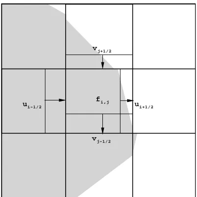
ford= 1. . .N (8) are solved sequentially for progressive updates of f for each of the N spatial dimensions. By treating only one velocity component at a time, the calculation of the advected volume fraction through each face can be analytically determined with relative ease, even for planar surface reconstructions in three dimensions (Scardovelli and Zaleski 2000). A typical two-dimensional recon-struction is shown in Figure 1. In this figure the velocities are scaled by ∆t/∆x making them local Courant numbers. With this scaling a donating region upwind of each face can be defined with width equal to the velocity magnitude. The dark fluid within each region will be fluxed into the next cell. In Figure 1, the fluid in the bottom-right corner of cell (i, j) is in two donating regions. To avoid the possibility of fluxing the same fluid into two different cells the surface must be reconstructed after each sweep of an operator-split method.

vj+1/2

ui+1/2

vj-1/2 ui-1/2

fi,j

Figure 1: 2D diagram of a typical linear VOF surface reconstruction on a 3x3 block of cells with scaled velocity components. Using the standard operator-split treatment, the donating regions are right-cylinders upwind of each face.

ensure that (6) is met after each step of the algorithm. In Figure 1 more fluid is being fluxed in from cell (i−

1, j) than space left after fluxing out to cell(i+ 1, j), meaning that cell(i, j)would overfill in the first sweep. Scardovelli and Zaleski (2003) investigate this effect in detail geometrically and develop a fairly simple two-dimensional operator-split Eulerian implicit Lagrangian explicit (EI-LE) method which conserves the global volume fraction exactly. In that method, (8) is integrated implicitly with ford = 1and explicitly with Lagrangian flux treatment ford= 2. Using the same velocity scaling as above, the discrete form of the implicit and explicit integrations are given by

f_i,jn+1/2=f

n i,j−

³ Fn

i+1/2−Fi−n1/2

´

h 1−un

i+1/2−uni−1/2

i (9)

f_i,jn+1=f_i,jn+1/2 h

1 +vn

j+1/2−vj−n 1/2

i

−

³

Gn_j+1+1_//₂2−Gn_j−+1_1//₂2 ´

(10) whereF andGare the fluxed dark fluid in the first and second directions. Puckett et al. (1997) propose the same

splitting without the Lagrangian flux calculation. Rider and Kothe (1998) propose integrating first explicitly, then implicitly.

Aulisa et al. (2003) demonstrate by two-dimensional algebraic mapping that the EI-LE scheme is the only one of the three that is volume conserving. It also shows that this is dependant upon a strictly two-dimensional divergence free velocity field. The mathematical analysis in that work is straightforward but does not help suggest a general solution for three-dimensional flows.

Breaking the problem of conservation into a short list of requirements clarifies the issues. Given that

1.The flux terms are conservative, and 2.The divergence term sums to zero and

3.No clipping or filling of a cell is needed due to violation of (6) at any stage

then the algorithm must conservef to machine precision. The first requirement ensures that any fluid going into one cell is coming out of another and the second ensures that there is no net source term added to the advection equation. Along with the third requirement, it is then guaranteed that there is no net change in f in the fluid domain regardless of the dimensionality of the system. By multiplying the divergence term byfn _{in the explicit} step and thenfn+1_{in the implicit step, Rider and Kothe}

(1998) create a net source term, violating requirement 2. Implicit integration violates requirement 1 by scaling the fluxes by a local stretching term, bracketed in (9). This scaling term is not consistent on both sides of the cell face, meaning the effective flux is not conservative. The EI-LE scheme maintains global conservation despite this by using the Lagrangian flux calculations and relying on the bracketed term in (9) to be exactly canceled by the bracketed term in (10) due to two-dimensional continuity. This cancelation is not extendable to three dimensions.

However, these requirements are not insurmountable and a simple operator-split algorithm which meets them is

fa_=fb_−∆

same fluid twice. The key features of this scheme are the use of conservative fluxes and the constantgnfield multi-plying the divergence term. Thus requirements 1 and 2 are met, and it only remains to examine requirement 3.

The form of (11) emphasizes that the divergence correction term is offsetting the dark fluid flux with an approximate flux proportional to the stretching. A definition of g is needed which maintains (6) for any configuration, and we propose the simple form

gn≡

½

1 if fn>1/2

0 else (12)

makingg a sharp version of f. It might seem intuitive to letgn =fn, but setting the approximate flux propor-tional to the fraction in the central cell does not guarantee conservation. Scardovelli and Zaleski (2003) give a detailed example of this for essentially the situation in Figure 1. Usinggn_=fn_{for this case results in overfilling} in the first step because the dilatation is small and the in-flux is large. Using the definition ofgabove enhances the influence of the stretching term and with the restriction

|ud|,|∆dud|< 1

2N −2 for alld (13)

guarantees that (6) is met at all stages of the algorithm. The velocity restriction limits the acceptable time step; yet our experience has shown that it is conservative, particulary for three-dimensional flows.

Even with the restriction on the time step, all three requirements are met and the algorithm will conserve volume fraction to machine precision. A series of canonical three-dimensional simulations were run to verify this capability and quantify errors in other methods. The test case is a high amplitude standing air-water wave and the Cartesian-grid solver described in the previous section was used to run the tests. The computational domain is a cube, with∆x/L = 0.025,∆t/T = 0.005

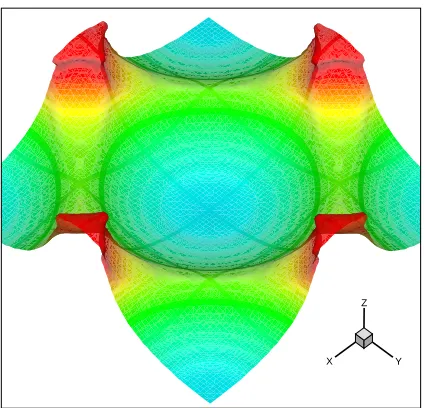
and reflection boundary conditions set on all walls. A sinusoidal free surface with A = 0.3L, λ = 2L and an average elevation of z = 0.5L is used as the initial condition. The slope is well above the Stokes limit and results in a highly nonlinear fully three-dimensional wave with overturning as seen in Figure 2.

Five advection methods were tested, the first being a baseline test with no stretching term included. The second two are extensions of methods such as that of Rider and Kothe (1998) to three-dimensional flows. The first (E-E-E) uses all explicit integrations of the form of (10) and the

X Y

Z

Figure 2: Visualization of the free surface for the 3D wave test att= 0.5. Contours indicate elevation. The nonlinear wave has nearly impinged on the top of the computational domain in this image.

second (I-I-E) uses implicit integration of the form of (9) for the first two steps. Next is the current method usingg as defined in (12) and then usinggn=fnfor comparison. The results are shown in Table 1. The first two columns give the L1andL∞ norms of the global volume loss in the domain after each use of the advection method. The third column gives the percentage change in total water volume in the domain after one wave period. The baseline gives by far the worst performance, with a net mass loss of 12% after only one wave period. The second and third rows show around an order of magnitude decrease in error compared to neglecting the stretching term altogether but still leave room for improvement.

The current method demonstrates nearly exact conser-vation of mass after each step and overall. The average values of|u|maxand|∆u|maxat the interface are around

Algorithm L1norm L∞norm % Change Baseline 2.53e-3 1.40e-2 -12.63%

E-E-E 3.03e-4 2.51e-3 -1.42%

I-I-E 1.22e-4 1.34e-3 +0.81%

Current 1.34e-12 6.83e-12 -0.00%

gn_=fn _{9.69e-6 1.51e-4 +0.04%} Table 1: Global mass loss measurements for a high slope 3D standing wave test case. The first two columns refer to the volume loss at each step, and the final column gives the total change after one wave period.

EXIT CONDITION

Exit conditions are required for external incompressible flow simulations and are notoriously difficult to enforce accurately. In practice poor exit conditions require large computational domains and short simulation times to avoid corrupting the solution. This reduces the compu-tational efficiency and reliability of the simulation. In this section a new exit boundary condition is presented which minimizes reflections for general fluid systems.

Unlike the free surface or a no-slip wall, an “exit” is a purely numerical boundary. The ideally semi-infinite domain of an external flow is truncated by the exit boundary to make the solution trackable. In estab-lishing an exit boundary, we are inherently assuming that the flow phenomena of interest are within the numerical domain and independent of the flow beyond the exit. Exit conditions must be set despite this assumption of independence because the pressure Poisson equation is elliptic and requires information on every boundary to ensure a globally divergence-free velocity field.

One method of modeling an exit is to construct a numerical beach to absorb the energy out of exiting waves. Such methods are often ineffective and require large buffer regions, lowering computational efficiency. In Dommermuth et al. (2004) a body force method is developed to drive the flow at the exit to match the free stream conditions, and Ferziger and Peric (2002) suggest using 1D extrapolation to set the velocity profile at the exit. While these methods can be applied in limited cases they rely on a strong underlying convective flow to wash away the errors resulting from their modeling inaccu-racies.

A more advanced unsteady condition is a wave exit, such as developed by Orlanski (1976). The typical

Orlanski-type boundary condition applied to the velocity

vector is _µ

∂ ∂t+c

∂ ∂x

¶

~u= 0 (14)

where c is the, as yet undetermined, wave speed and the x-coordinate represents the direction normal to the exit. When using this condition, the mass flux through the boundary is prescribed and a compatible Neumann condition must be set on the pressure. Reasonable choices of the wave speedcare the free-stream velocity or some other natural velocity metric, such as √gL. In Hurt (1999), a field of exit speeds are determined by solving (14) for c one point interior to the exit. However, this method is unstable if the momentum equations are integrated explicitly.

Regardless of how the wave speed is chosen, if there are multiple waves with differing speeds exiting the domain, (14) will produce reflections for waves with speeds not equal toc. The Higdon condition (Higdon 1994) has been developed to circumvent this difficulty. The condition is a wave product

HJ : J

Y

j=1

µ ∂

∂n+

1

cj

∂ ∂t

¶

~u= 0 (15)

wherecj are the set of exiting wave speeds. Increasing the number of wave speeds reduces the energy reflected back into the domain. Derivation and implementation of this conditions for the two-dimensional wave equation is given by Givoli et al. (2003), but applying this boundary condition to incompressible free-surface flows is nontrivial.

Formally, this adjustment to the x-component of the velocity vector can be written as

µ ∂ ∂t+c

∂ ∂x

¶

u=−α (16)

whereαis some, hopefully small, deviation from a true exiting wave form. The terms above are readily correlated to those of thex-component of the momentum equation

µ ∂

∂t+~u·∇~ ¶

u=−1

ρ ∂p

∂x. (17)

The time derivatives match andc∂u_∂x is a one-dimensional model of the convective acceleration. The remaining term is the pressure force, which leads us to formulate a boundary condition of the form

µ ∂ ∂t +c

∂ ∂x

¶

u=−1

ρ ∂p

∂x (18)

for the exiting component of velocity. Adjusting the standard Orlanski exit in this way allows the pressure field to fulfill it’s normal role of projecting the velocity onto a solenoidal field. Therefore, no global flux integrations are required and the system will conserve mass locally and globally to the tolerance of the pressure solver.

When using (18) a Dirichlet boundary condition must be set on the pressure equation. Hydrostatic pressure could be set at the exit, but a wave condition for the

pressure _µ

∂ ∂t+c

∂ ∂x

¶

p= 0 (19)

is the most consistent option. The boundary condition is applied at the exit using linear interpolation

Pe= 1

2(PE+PI) (20)

wherePe is the interpolated exit value and PE andPI are the cell-centered values to the exterior and interior of the exit respectively. Second-order central differences and Runge-Kutta integration in time then give the boundary equations as

Pn_e+1/2=Pn_e−c∆t

∆x (P

n

E−PIn) (21) in the predictor step and

Pn_e+1=1 2 h

Pn_e+Pn_e+1/2

−c∆t

∆x ³

P_En+1/2−P_In+1/2 ´i

(22)

in the corrector step. These equations are substituted into the pressure equation to eliminate references to the exterior pressure value. While modifying the pressure equation at the exit in this manner does entail some additional complexity it is the only method presented which can be used to model any general free-surface flow. To quantify the performance of these exit condition a series of tests are run using two-dimensional Cauchy-Poisson waves. The domain has an aspect ratio of 2 and is discretized using∆x/L = 0.04and∆t/T = 0.02. The exit conditions are set on the far right boundary atx= 4L

and free-slip conditions are set on all other boundaries. The initial free-surface elevation is set toη(x)/L= 1 +

1

2exp(−πx/L). To measure the error induced by the exit,

a reference solution is generated by doubling the length of the numerical domain and using the standard Orlanski exit withc = 1.5L/T atx= 8L. Figure 3 shows the initial condition from x = 0..4L along with subsequent snap-shots in a waterfall plot for this reference solution. In this figure, time progresses by moving down the page, and the waves travel from left to right. Four nonlinear waves of decreasing amplitude, wavelength and speed can be easily identified in the figure. The figure also shows that there is little reflection into the domain during this time period justifying our use of this solution to estimate errors in the simulations on the truncated domain.

Four types of exiting conditions are tested, the first of which is a baseline case using a free-slip wall condition. This condition will give pure reflection. The second exit condition uses linear extrapolation to determine the velocity profile at the exit. The u component was corrected in by global flux integration to ensure mass conservation. The third condition is the standard single-speed Orlanski exit described by (14) using a global integration adjustment to determineα. The last condition is the pressure adjusted wave exit using (18) and (19). The wave speed is set toc = 1.5L/T for all the wave cases. Figure 4 shows the results from all of these tests along with the reference solution as the second wave reaches

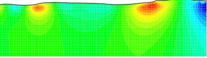
x= 4Latt= 3.36T. Contours of ∂p_∂x are plotted within the water to aid in comparing the methods. By this time, the large first wave has reflected back across the domain in Figure 4(b) and the comparison to the reference solution is already poor. The extrapolation exit condition is observed to give essentially the same solution as the reflection exit. The two wave exits compare much better to the reference solution.

x

0 1 2 3 4

t = 1.92 s t = 0.48 s

t = 0.96 s

t = 1.44 s t = 0.0 s

t = 2.88 s t = 2.40 s

t = 3.36 s

t = 3.84 s

Figure 3: Free surface elevation waterfall plot of the reference solution. Each line is6∆t = 0.12T later than the line above it. The view is truncated at the x = 4L where the tested numerical exit conditions were enforced.

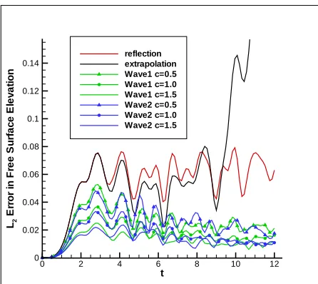
of the error in the free surface elevation in the truncated domain is calculated as a function of time. The results are shown in Figure 5 for each exit condition and for a range ofc values. The error in the pure reflection condition is seen to fluctuate in time as the waves reflect from one end of the truncated domain to the other. The Euler equations generate no physical dissipation to damp out the wave energy yet the magnitude of error remains well bounded in time. This is in contrast to the extrapolation exit which has similar characteristics to the reflection boundary initially but rapidly becomes unstable and diverges completely at

t= 9T. This instability in the extrapolation exit demon-strates that spurious information generated at the exit has fully corrupted the solution.

The next six lines of Figure 5 show the wave exit with global-integration correction (labeled Wave 1) and pressure correction (labeled Wave2) using wave speeds of c = 0.5,1.0 and 1.5L/T. All six wave exits show a significant decrease in error and a fast overall trend towards zero error in time. By t = 10T nearly all waves have traveled out of the truncated domain, and the remaining error is likely indicative of reflections in the reference solution. For all choices of wave speed, we see that the pressure corrected exit has comparable errors to the exit corrected by global-integration. As (18) is more

(a) Reference solution

(b) Reflection condition

(c) Extrapolation exit

(d) Wave exit with global-integration adjustment

(e) Wave exit with pressure adjustment

t L2

E

rr

o

r

in

F

re

e

S

u

rf

a

c

e

E

le

v

a

ti

o

n

0 2 4 6 8 10 12

0 0.02 0.04 0.06 0.08 0.1 0.12 0.14

reflection extrapolation Wave1 c=0.5 Wave1 c=1.0 Wave1 c=1.5 Wave2 c=0.5 Wave2 c=1.0 Wave2 c=1.5

Figure 5: Measurements of theL2 spacial norm of free

surface error as a function of time. The wave exit with global-integration correction are labeled Wave 1, and the pressure corrected exits are labeled Wave 2.

physically relevant than (16) and allows comprehensive treatment of free-surface flows, we conclude it to be a significant advancement.

However, the measurements shown in figure 5 still show reflections which could corrupt solutions. The Higdon condition may be used to extend the method to multiple wave speeds but solution algorithms for such methods are complicated, particularly for variable density flows. Simplifying these numerical methods is a topic of current research.

BODY BOUNDARIES

Treatment of body boundaries are of particular concern in Cartesian-grid methods. The methods currently available have limitations in applications or accuracy or have complicated implementations. A general framework is presented in the next two sections to formulate equations of motion which accurately simulate complex flows around solid geometries. A simple implementation is proposed which automatically maintains the order-of-accuracy of the general flow solver. While any surface representation could be used with this method, we present a representation which increases ease of use and efficiency.

Thus far, two primary methods exists in the literature to enforce the effects of solid bodies in Cartesian-grid simulations: Immersed-Boundary methods and Cut-Cell methods. The Immersed-Boundary method was developed for use in fluid-structure interaction problems, specifically biological fluid dynamics. Peskin (2002) gives a detailed review. In general, the elastic body equations are solved on an explicitly defined surface mesh, while the fluid equations are solved on a Cartesian grid. The two simulations are linked by applying the reaction force of the body on the fluid and advecting the body in the resulting flow. The localized forces and body velocities are calculated using a smoothed approximation of the Dirac delta function. Because the body is advected by the flow the interactions are restricted to flexible bodies and systems that are not mathematically stiff.

The so called Cut-Cell methods alter the discrete form of the fluid equations of motion near the body to account for its presence. There are a great variety of these methods, and the body may either be explicitly defined by a mesh or implicitly defined by a field (Udaykumar et al. 2001). The changes to the discrete equations often involve interpolating boundary values such as in Chimera methods and altering the local grid metrics such as with non-orthogonal grids. Other alterations have also been researched such as locally changing the grid from staggered to collocated (Gilmanov and Sotiropoulos 2005) and setting up extrapolated “ghost-cells” (Tseng and Ferziger 2003) within the domain. The diffi-culties with these methods are their complexity, compu-tational expense and maintaining the flow solver’s order of accuracy and stability (Ye et al. 1999).

Dommermuth et al. (1998) avoids these issues in developing a simple body force method suitable for rigid no-slip bodies such as ships. A body force term is added to the discrete momentum equations within the body proportional to the velocity error. This force drives the velocity of the fluid within the body to the prescribed body velocity exponentially in time. As such, the boundary condition is treated as a goal-state rather than an instan-taneous restriction on admissible velocity fields.

delta function, or switch function, defined as

δ0_(~x)≡

½

1 for all ~x∈ B

0 else (23)

is used to alter the analytic form of the governing equations. This is in contrast with Cut-Cell methods which change the discrete form of the equations near the body. By directly imposing constraints on the velocity field the body will drive the flow instead of being advected by it, allowing for the treatment of high-stiffness bodies such as ship hulls.

No-Slip Condition

In this subsection equations to enforce the no-slip body boundary condition on a general topological body B

immersed in the fluid domainRare derived. We are given the velocity vectorU~ ofBas well as the distance from any fluid point in the domain to the body surface. The no-slip condition is then stated as

~u=U~ for all~x∈ B. (24) To derive a no-slip equality for use in the momentum equation, (24) is substituted into (2) to give

∂ ~U

∂t +

1

ρ∇~p−~r= 0 for all~x∈ B, (25)

which is commonly used as a starting point for deriving solid-body boundary conditions for the pressure. In this method we instead multiply (25) by the function δ0_{. Its} definition ensures that this product is zero throughout the domain and therefore may be added to (2) resulting in the altered momentum equation

∂~u

∂t = (1−δ

0₎

µ ~r−1

ρ∇~p ¶

+δ0∂ ~U

∂t. (26)

Taking the divergence gives the corresponding pressure equation as

~

∇·

µ 1−δ0

ρ ∇~p ¶

=

~

∇ ·

Ã

(1−δ0)~r+δ0∂ ~U

∂t −

∂~u ∂t

!

. (27)

Equations (26) and (27) are identical to equations (2) and (3) except on B where the switch function is

used to transition the equations to an enforcement of the no-slip condition. Technically speaking, the above equations enforce the time derivative of (24), but when the momentum equation is integrated in time, the exact boundary condition is recovered on B. This analytic transition from the field equations to the boundary conditions differs significantly from the standard body force or Immersed-Boundary formulations.

When these equations are applied to the boundaries of the numerical domain, they produce exactly the same discrete formula obtained by applying boundary conditions to a boundary fitted grid. This demonstrates that equations (26) and (27) are generalizations of the equations used in fitted grid methods, allowing the body to lay anywhere in the domain instead of restricting it to coincide with the domain boundary. Because of this generality the above equations can be formulated for any number of arbitrary bodies with any given velocity. Also, as B need not be a material surface, the inflow and outflow boundaries can be modeled with this formulation by settingU~ appropriately.

No-Penetration Condition

The method is next extended to the no-penetration condition, given by

~u·~n=U~ ·~n for all~x∈ B (28) where~nis the unit normal vector of the surface ofB.

This boundary condition is substituted into the normal projection of (2) to give

" ~n·

à ∂ ~U

∂t +

1

ρ∇~p−~r !

+∂~n

∂t · ³

~ U−~u

´# ~n= 0

for all~x∈ B (29) where the second term within the brackets is arbitrary and can be set to zero. To see this, note that the length of

~n is constant, meaning its time derivative must lies in the tangent plane to the body surface. As the tangential velocity ofU~ is arbitrary it can always be set so that the inner product vanishes.

Using the same procedure as in the previous section, (29) is multiplied by δ0 and added to the governing equations. The resulting no-penetration momentum and pressure equations are

∂~u

∂t = (I−δ

0_N)

µ ~r−1

ρ∇~p ¶

+δ0_N∂ ~U

and

~

∇·

µ

(I−δ0N)1

ρ∇~p ¶

=

~

∇ ·

Ã

(I−δ0N)~r+δ0N∂ ~U

∂t −

∂~u ∂t

!

, (31)

where I is the identity tensor and N ≡ ~n~n is the normal dyad. Although similar in form to the no-slip equations, the no-penetration equations feature tensor products instead of simple multiplication. This additional complexity arises because (28) is a scalar equality and can therefore only make a rank-one adjustment to the governing equations. The adjustment is made through the rank-one dyad N, leaving the (N − 1) tangential components of the momentum equation unchanged by the presence of the body. These tangential equations are then free to carry any user defined slip model including the no-slip condition. This topic is explored further in the following sections.

The tensor products make numerical solution of the no-penetration equations more laborious. The source term of (31) is easily constructed, but the Poisson coefficients give rise to cross derivatives. These cross derivatives are needed to cancel out the normal component of the pressure gradient. As they arise in this general formu-lation they must be treated regardless of the implemen-tation being Cut-Cell, fitted-grid, or the method described in the next section. In this work, the cross derivatives have been treated with differed-correction whereby old values of the cross derivatives are used and then corrected after the pressure field is calculated. This maintains the simplicity of the pressure solver and allows general treatment of the equations throughout the domain. Numerical Implementation

In a flow solver the momentum equation is evaluated at discrete points in the domain which, in general, do not exactly coincide with the surface B, allowing the surface to “hide” from the flow. There are many ways to overcome this issue, the best established of which is to use a non-orthogonal boundary-fitted grid. Another option is to alter the discretization of the momentum and pressure equations near the body, as in Cut-Cell methods. An example is the slip condition presented in Dommermuth et al. (2005), which is derivable by integrating (31) over each finite volume.

In this work a smoothed approximation of the analytic delta will be used instead of altering the discretization scheme. Similar to the form used by the Immersed-Boundary method, we define the smoothed switch function as

δ0_{(~x) =}

½ ₁

2

¡

1 +cos¡dπ ²

¢¢

for all |d|< ²

0 else ,

(32) wheredis the distance from the point ~xto the surface, and²is the width of the numerical delta function. This definition is used to allow modeling of thin sheets in our solver. An alternate definition more akin to the smoothed heavy side function would be appropriate for thick solid bodies. Because of the use of (32), discon-tinuities resulting from the presence of the body will be smoothed over the width ². The current method is therefore not a “sharp-interface” method, and care must be taken in the setting of ² such that accuracy is not lost. The smoothing width was set to ² = 2∆x√N for all tests in this work and is demonstrated below not to reduce solution accuracy. The benefit of this method is its trivial and general implementation. Also, because the method does not alter the calculation of derivatives the order-of-accuracy of the bulk flow solver is automatically maintained.

Two simple tests are presented to demonstrate the ability of this boundary condition enforcement technique to accurately simulate unsteady free-surface flows. In both, a two-dimensional tank with aspect ratio 2 is simulated using ∆x = 0.0125L and∆t = 0.00267T. The first case is a high amplitude standing wave test with

A= 0.2Landλ=L. An image of the resulting nonlinear wave at timet=T is shown in Figure 6(a). Note that the simulation is symmetric on either side of the x= 0.5L. To test the proposed method a vertical wall is placed at that location and a constant free surface height of0.05L

is set on the right side while the wave initial condition is maintained on the left. This simulation will thus test the method’s ability to enforce the no-penetration condition and quantify the errors due to smoothing the boundary. The result using the current method is shown in Figure 6(b). For comparison the result for the same simulation using the body force method is shown in Figure 6(c). Unlike the body force method, no fluid is transmitted through the wall, and errors due to smoothing are very small.

quickly displaced to the right by 0.2L and then held steady. This can be modeled using a frame of reference that moves with the tank, accounting for the acceleration by the application of a uniform body force. It can also be simulated by enforcing the no-penetration condition on the moving vertical walls of the tank using a stationary frame of reference. Therefore, the same result should be generated using a fitted grid or moving immersed boundaries, allowing for a direct comparison. Figure 7(a) and 7(b) show the result for the fitted and immersed grid respectively at t = 2.4T. The images show that the comparison between the methods is excellent, even for this highly complex flow with dynamic boundaries. Advanced Body Representation

All flows with bodies must describe the geometry in some way and the most useful description is problem dependant. When solving biological fluid-dynamics problems with the Immersed-Boundary method, a simple algebraic mesh representation is logical because the elastic body equations need to be solved on a mesh. However, when solving flows with the method described in the previous section a more powerful set of functions can be chosen to describe the geometry.

NURBS (Non-Uniform Rational B-Splines) are one of the most popular tools used to represent lines and surfaces in computer aided design and graphics, and are the backbone of such programs as Rhino and FastShip. This is because of their efficient implementation, their intuitive control point interface, and the smoothness properties of the resulting forms. In this work, the NURBS description used to design a solid body is maintained in the computational analysis of the flow around that body. This eliminates all need for gridding and assures the designer that WYSIWYG1_{. Another consideration is that}

NURBS surfaces have far fewer parameters than algebraic grids making them better suited for shape optimization problems.

In order to enforce body boundary conditions on a Cartesian grid every point on the grid must know the distancedto the nearest point on the body. Additionally, topological parameters such as the normal~nare required. Although nowhere near as time consuming as creating a fitted mesh, determining these values can be a slow process. On an algebraic mesh the distance to the body is found by an exhaustive search of every point, line,

1_{What You See Is What You Get}

(a) Symmetric standing wave in full tank

(b) Standing wave in split tank using current method

(c) Standing wave in split tank using body force method

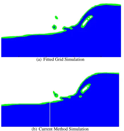
(a) Fitted Grid Simulation

(b) Current Method Simulation

Figure 7: Image of sloshing waves in a tank generated by rapid sideways displacement using the same coloring as in Figure 6. Figure (a) shows the baseline using a fitted-grid formulation and Figure (b) shows the result using the current method.

and planar surface on the mesh. The parametric NURBS representation allows the use of a gradient based search for the distance function that is orders of magnitude faster. Formulating the squared distance from a point ~xin the domain to the pointX~ on the body as a function of the surface parameter~sas

ψ2_{(~s) =}¯¯_{¯~x−X~(~s)}¯¯_¯2_{, (33)}

allows the minimum distance function to be defined by

d2= min

~s ψ

2_{(~s) (34)}

which can be solved with the Gauss-Newton method for non-linear least squares which has a second-order convergence rate.

To quantify the speed-up observed by using this method, the signed distance function and normal vector for a spherical test geometry are computed on a series of background grids. This is compared to the average accuracy and speed of calculation of the distance function

R/∆x NURBS time Mesh time Mesh Error

32 0.301e-1 0.201e-1 0.119e-2

64 0.121e+0 0.660e+0 0.178e-3

128 0.181e+1 0.202e+2 0.453e-4

256 0.127e+2 — —

Table 2: Distance calculation statistics for immersed sphere using mesh and NURBS based surface represen-tations.

and normal using a structured surface mesh. Table 2 shows these results. The distance function and normal vector were found using a single processor computer, and the times (given in seconds) are only meant for relative comparison. The valueR/∆xis the sphere radius over the grid spacing and therefore proportional to the number of grid points in one direction. The average error in the parameters using the NURBS solver was less than 1e-7. The mesh-based method was stopped after 45 minutes on the finest grid and the results are not shown for this case. The table shows that the cost of determining the parameters scales linearly with the number of points when using the Gauss-Newton solver, but at least quadratically when using an exhaustive search on the mesh. This is especially important when the geometry is continually changing as the simulation progresses, such as in hull shape optimization and the flexible wave maker problem presented in the next section.

An additional advantage of this representation is that it can be easily adjusted to compute distance function to the cross-sectional lines of any surface. When the distance function is found using a gradient method a lagrange multiplier can be constructed which constrains the set of admissible points on the surface to a particular cross section with no increase in computing time. To create the same distance function using a meshed geometry would require expensive and complicated preprocessing of the body geometry. Figure 8 shows a containership bow with the cross sectional lines. Though the lines are discon-tinuous at the bulbous bow the current method can handle this discontinuity with no special treatment.

NAVAL SHIP HYDRODYNAMICS APPLICATION

Figure 8: Bow of a general containership hull-form with bulb. The lines are cross sections of the surface withx -planes, as would be required for 2D+t simulation.

methods to simulate flows with naval applications and use comparisons of those solutions to experimental results to discuss possible reduced models of bow flows and proper tangential boundary conditions for Cartesian-grid methods.

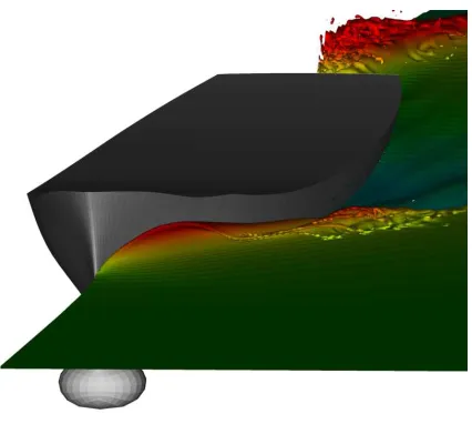
Figure 9 shows the bow wave flow of the model 5415 hull in a 30 knot simulation generated using standard NFA methodologies. This simulation is preformed on massively parallel machines using nearly 30 million grid points and grid stretching on the Cartesian mesh. Comparison of these simulations to experimental results for the same test case demonstrate generally good agreement, but the experiments show that the run-up of the bow wave is under-predicted by NFA even for this high resolution run. This error is due to the seven orders of magnitude disparity in relevant length and time scales in naval ship hydrodynamics which can not be resolved directly even with the most advanced brute force methods (Weymouth et al. 2006).

One interesting proposal to deal with the demands of resolving full-scale naval hydrodynamic flows is to adopt the “slender ship” assumptions, modeling the three-dimensional system as a 2D+t flow. 2D+t models simplify the simulation of ship bow waves by assuming that changes in the longitudinal direction are small compared to changes in the transverse directions. Historically, this allowed potential flow simulations of the bow waves around slender vessels to be generated with orders of magnitude savings in computational expense. Fontaine et al. (2000) provide a thorough derivation of the method and present results generated using a nonlinear potential

Figure 9: 3D image of the 5415 bow wave flow at 30 knots as simulated by NFA

flow solver.

The pertinent issues may be addressed with a brief introduction to the 2D+t methodology. Using the ship length L and draft D as the relevant dimensional parameters gives the laplace equation for the velocity potentialφclose to the body as

µ γ2 ∂2

∂xˆ2 +

∂2

∂yˆ2 +

∂2

∂zˆ2

¶

φ= 0 (35)

wherexˆ =x/L,yˆ=y/D,zˆ=z/Dandγ =D/L. If the vessel is very slender then γ ¿ 1 and the equation has no x-dependance to leading order. The kinematic and dynamic free-surface boundary conditions set the requirement that

γU2

gL ÀO(1) (36)

and impose a downstreamx-dependance on the solutions, but no upstream influence (Fontaine and Cointe 1997). Therefore, the problem is parabolic and may be posed as an unsteady two-dimensional nonlinear system instead of a three dimensional one.

not be assumed that the flow is inviscid. Additionally, plunging breakers such as those of Figure 9 are highly rotational. Therefore, a potential function may not be used to describe the velocity field and other means must be used to simulate the flow within this 2D+t framework.

Geometrically, the 2D+t assumptions reduce the three-dimensional fluid problem to a two-three-dimensional cross section of the flow which moves along the length of the body in time. This models the hull as a deforming curve which can be though of as a flexible wave maker, pushing out the 2D+t representation of the divergent wave system generated by the body. Shakeri (2005) presents experi-mental results for a physical realization of this geometric interpretation. In those experiments, a large (3m tall) wave maker was actuated by hydraulics to sweep out the bow of the 2D+t representation of a modified model 5415 hull traveling at 25 knots. The sonar dome was removed from the representation of that hull due to limitations in the wave maker experimental apparatus. This shows that while these experimental results bypass the limitations of potential flow they introduce limitations of their own.

Cartesian-grid methods overcome these shortcomings and those of potential flow and afford the opportunity to study the effect of 2D+t modeling on breaking bow waves generated by realistic ship geometries. As depicted in Figure 8, hulls with bulbs, chines and appendages hulls give rise to discontinuous and multiply connected “wave makers” that only the NURBS body represen-tation and Cartesian-grid methods have the capability of modeling simply and generally. Such hull features will generally violate the slenderness assumptions of the 2D+t framework, and the errors incurred by these effects can be quantified with detailed simulations.

Additionally, Cartesian-grid methods offer the unique capability to quantitatively determine the bounds on the validity of 2D+t models for complex bow flows. 2D+t methodologies demand that a hull with lengthLand speed

U will produce the same wave as a stretched geometry with length 10L and speed 10U. A series of three-dimensional simulations can be run varying the length scale and Froude number of the vessel to determine when stream-wise variations become important. Because the methods proposed in this paper are general enough to model free surfaces, exits and bodies in two or three dimensions, comparisons of simulations with different numbers of dimensions can be made with confidence.

As a first step the data provided by Shakeri (2005) is used to validate the Cartesian-grid capabilities described

x

y

1 2

0.5 1 1.5 2

Figure 10: Image of the flexible wave maker and calculated flow on the finest grid. The dark solid line is the wave maker surface, the arrows are velocity vectors and the blue coloring denotes water. Every third velocity vector is shown for clarity. The no-penetration condition is enforced on the body

in the previous section. The wave maker is simulated with the body treatment of the previous section and the position of the wave maker in time is set to exactly duplicate the experimental conditions. A computational domain of3mby6mis defined for the simulations and a series of time steps and grids spacings are used to judge their influence on accuracy. Coarse, medium and fine background grids with spacings of∆x= 0.04m,0.028m and0.02mrespectively are used. The pressure corrected wave exit developed above is used withc = 1m

s. Figure 10 shows a snap-shot of the wave maker and simulated flow using the no-penetration condition on the finest grid level. As can be seen from the velocity vectors in that image, the wave maker is sweeping from left to right with the lower end pined. In this simulation, fluid was allowed to flow in behind the wave maker using a one-way periodic condition, ensuring that the continuity condition is met in that region. The flow behind the wave maker has no influence on the flow exterior to the wave maker. The image demonstrates that the fluid has been allowed to run smoothly up the side of the body boundary and that the no-penetration condition has been exactly enforced in the normal direction.

t/T

z

/D

0 0.1 0.2 0.3 0.4 0.5

0 0.1 0.2 0.3 0.4

Experiments No-Slip BC: Fine No-Pen BC: Fine No-Pen BC: Medium No-Pen BC: Coarse

Figure 12: Experimental and simulated wave maker free surface contact lines. Coarse, medium and fine background grids use spacings of∆x= 0.04m,0.028m

and0.02mrespectively.

breaking events. Note that the two-dimensional nature of this simulation does not allow the breaking wave to fully close and the plunger instead skips off of the free surface. Because the no-penetration condition has been used, the point of contact between the free surface and the wave maker moves freely in this simulation, raising nearly

0.4m at it’s peak. Figure 12 shows the experimental measurements of the point of contact on the wave maker surface along with four sets of simulated results. The free surface run-up is denoted (z) and is normalized by the wave maker depth (D). The figure shows that all of the simulations have good general correlation with the exper-imental measurements. In particular, the no-penetration conditions accurately predict the rates of up and run-down compared to the measurements for all resolution levels, but they overshoot the maximum height substan-tially. In contrast the no-slip condition accurately predicts the run-up and maximum height but the run-down is much too slow, leaving the hull wetted for longer than the exper-imental result. The no-slip result shown in Figure 12 is for the finest grid only. The coarse and medium grid simulations did not sufficiently resolve the near-wall flow to give accurate results and have not been shown.

The results of Figure 12 and practical limitations on computational resources suggest that a slip model must

be added to the no-penetration condition to model the effects of near-wall viscosity on this wave maker flow and its three-dimensional counterpart. Adding a slip model for the tangential equations of motion using the analytic development given in the previous sections is straight-forward and the momentum equation takes on the form

∂~u

∂t = (1−δ

0₎

µ ~r−1

ρ∇~p ¶

+δ0N∂ ~U

∂t +δ

0_{(I−N)K.~ (37)}

~

K is the user defined slip model which can be set as a function of fluid velocity, pressure, density, wall roughness, and any other pertinent parameters. (37) is the most general slip model formulation with proper choice ofK~ recovering the no-penetration and no-slip conditions and many possibilities between.

A promising compromise between the no-penetration and no-slip condition is to use a body force correction similar to that developed in Dommermuth et al. (1998) to model the tangential flow. In that formulation, K~

would reintroduce the tangential momentum equations and include a body force term proportional to the slip velocity at the body surface. The force is scaled by a friction coefficient and in Dommermuth et al. (1998) that coefficient is set very high to enforce the no-penetration condition on the hull. However, used in the framework of (37) the coefficient could be tuned based on experimental evidence such as shown in Figure 12. More detailed experimental measurements and numerical studies will allow further investigation of this slip condition, with the goal of a simple and general formulation for free-surface flows.

x

y

1 2 3

0.6 0.8 1 1.2 1.4 1.6 1.8 2 2.2

Figure 11: Multiple exposure image of the flexible wave maker and calculated free surface on the finest grid. The black lines are the wave maker surface, and the blue lines are the contours off = 0.5. The no-penetration condition is enforced on the body.

CONCLUSION

This work has shown that Cartesian-grid methods are capable simulating flows with engineering appli-cations without the difficulties associated with fitted-grid methods. New capabilities have been developed to further extend the usefulness and generality of Cartesian grid methods. A free surface advection algorithm which conserves the volume of fluid at the interface even for complex three-dimensional flows has been presented. Exit boundary conditions for the velocity and pressure have been derived which allow for accurate simulation of general external flows. A body boundary formulation based on the analytic alteration of the governing equations has been presented which allows enforcement of general boundary conditions and is easily implemented such that the solver order of accuracy is maintained. A series of simulations of a flexible wave maker were presented which used all of these numerical advancements showed good comparison to experimental results. Specifically, the no-slip and no-penetration boundary conditions each captured elements of the physical system, and a more advanced tangential slip model will help improve the comparison further. An outline of a method to quantify

the bounds on the 2D+t slenderness assumptions were made and the need for a method to allow variation of flow in the air was introduced. With the capabilities presented in this paper highly accurate simulations of general ship flows are achievable.

This work was supported by the Office of Naval Research under grant N00014-01-1-0124 through Dr. L. Patrick Purtell. The computational resources for this work were provided through a Challenge Project grant from the Depart of Defense High Performance Computing Modernization Office (Project C1V). The authors wish to thank J. Duncan and M. Shakeri for the use of the experi-mental wave maker data.

REFERENCES

Aulisa, E., Manservisi, S., Scardovelli, R., and Zaleski, S., “A geometrical area-preserving Volume-of-Fluid advection method,” J. Comp. Phys., 2003, vol. 192, pp. 355–364.

Dommermuth, D.G., OShea, T.T., Wyatt, D.C., Sussman, M., Weymouth, G.D., Yue, D.K., Adams, P., and Hand, R., “The numerical simulation of ship waves using cartesian-grid and volume-of-fluid methods,” 26th Symposium on Naval Hydrodynamics.

Dommermuth, D.G., Sussman, M., Beck, R.F., O’Shea, T.T., Wyatt, D.C., Olson4, K., and MacNeice, P., “The numerical simulation of ship waves using cartesian grid methods with adaptive mesh refinement,” 25th Symposium on Naval Hydrodynamics.

Dommermuth, D.G., Sussman, M., O’Shea, T.T., and Wyatt, D.C., “The Numerical Simulation of Ship Waves using Cartesian Grid and Volume-of-Fluid Methods,” 26th International Conference Numerical Ship Hydrodynamics.

Ferziger, J. and Peric, M., Computational Methods for Fluid Dynamics, Springer, 3rd ed., 2002.

Fontaine, E. and Cointe, R., “A Slender Body Aproach to Nonlinear Bow Waves,” Phil. Trans. Royal Society of London, 1997, vol. A 355, pp. 565–574.

Fontaine, E., Faltinsen, O.M., and Coite, R., “New insight into the genertion of ship bow waves,” J. Fluid Mech., 2000, vol. 421, p. 1538.

Gilmanov, A. and Sotiropoulos, F., “A hybrid Cartesian/immersed boundary method for simulating flows with 3D, geometrically complex, moving bodies,” J. Comp. Phys., 2005, vol. 207, pp. 457–492. Givoli, D., Neta, B., and Patlashenko, I., “Finite element analysis of time-dependent semi-infinite wave-guides with high-order boundary treatment,” J. Comput. Phys., 2003, vol. 58, pp. 1955–1983.

Hendrickson, K. and Yue, D.K.P., “Navier-Stokes simulations of unsteady small-scale breaking waves at a coupled air-water interface,” 26th Symposium on Naval Hydrodynamics.

Higdon, R., “Radiation boundary conditions for disperive waves,” SIAM J. Numerical Analysis, 1994, vol. 31, pp. 24–462.

Hurt, C.W., “Addition of Wave Transmitting Boundary Conditions to the FLOW-3D Program,” 1999, vol. FSI-99-TN49.

Orlanski, I., “A Simple Boundary Condition for Unbounded Hyperbolic Flows,” J. Comp. Phys., 1976, vol. 21, p. 251.

Peskin, C.S., “The immersed boundary method,” Acta Numerica, 2002, pp. 1–39.

Pilliod, J. and Puckett, E., “Second-order accurate volume-of-fluid algorithms for tracking material interfaces,” J. Comput. Phys., 2004, vol. 199, pp. 465– 502.

Puckett, E., Almgren, A., Bell, J., Marcus, D., and Rider, J., “A high-order projection method for tracking fluid interfaces in variable density incompressible flows,” J. Comput. Phys., 1997, vol. 130(2), pp. 269–282. Rider, W.J. and Kothe, D.B., “Reconstructing Volume

Tracking,” J. Comp. Phys., 1998, vol. 141, pp. 112– 152.

Scardovelli, R. and Zaleski, S., “Analytical Relations Connecting Linear Interfaces and Volume Fractions in Rectangular Grids,” J. Comp. Phys., 2000, vol. 164, pp. 228–237.

Scardovelli, R. and Zaleski, S., “Interface reconstruction with least-square fit and split EulerianLagrangian advection,” Int. J. Numer. Meth. Fluids, 2003, vol. 41, p. 251274.

Shakeri, M., An experimental 2D+T investigation of breaking bow waves, PhD dissertation, Department of Mechanical Engineering, University of Maryland, 2005.

Tseng, Y. and Ferziger, J., “A ghost-cell immersed boundary method for flow in complex geometry,” J. Comp. Phys., 2003, vol. 192, p. 593623.

Udaykumar, H.S., Mittal, R., Rampunggoon, P., and Khanna, A., “A Sharp Interface Cartesian Grid Method for Simulating Flows with Complex Moving Boundaries,” J. Comp. Phys., 2001, vol. 174, pp. 345– 380.

Weymouth, G., Hendrickson, K., OShea, T., Dommermuth, D.G., Yue, D.K., Adams, P., and Hand, R., “Modeling Breaking Ship Waves for Design and Analysis of Naval Vessels,” DOD HPCMP Users Group Conference 2006.