University of New Orleans University of New Orleans
ScholarWorks@UNO
ScholarWorks@UNO
University of New Orleans Theses and
Dissertations Dissertations and Theses
5-14-2010
State Estimation with Unconventional and Networked
State Estimation with Unconventional and Networked
Measurements
Measurements
Zhansheng DuanUniversity of New Orleans
Follow this and additional works at: https://scholarworks.uno.edu/td
Recommended Citation Recommended Citation
Duan, Zhansheng, "State Estimation with Unconventional and Networked Measurements" (2010). University of New Orleans Theses and Dissertations. 1133.
https://scholarworks.uno.edu/td/1133
State Estimation with Unconventional and Networked Measurements
A Dissertation
Submitted to the Graduate Faculty of the University of New Orleans
in partial fulfillment of the requirements for the degree of
Doctor of Philosophy in
Engineering and Applied Science
by
Zhansheng Duan
B.S. Xi’an Jiaotong University, 1999 Ph.D. Xi’an Jiaotong University, 2005
Acknowledgments
This research was supported in part by NSFC grant 60602026, Project 863 through
grant 2006AA01Z126, ARO through grant W911NF-04-1-0274, NASA/LEQSF through
grant (2001-4)-01, ARO through grant W911NF-08-1-0409, ONR-DEPSCoR through grant
N00014-09-1-1169, and NAVO through Contract # N62306-09-P-3S01.
I would like to express my sincerest gratitude to my major advisor, Dr. X. Rong Li, for
his insightful and knowledgeable direction, continuous help and support, invaluable
encour-agement and discussion, the freedom allowed at doing research during the past four and a
half years and even before I came to the Unite States, which made the completion of my
current Ph.D. research work possible and will definitely benefit my career greatly.
I would also thank Dr. Tumulesh K. S. Solanky, Dr. Vesselin P. Jilkov, Dr. Huimin
Chen, and Dr. Dongxiao Zhu for serving on my thesis committee, and for their constructive
and valuable comments on the dissertation. Special thanks give to Dr. Li, Dr. Jilkov, Dr.
Chen, Dr. Zhihai He from University of Missouri, Columbia, and their families, Dr. Ning
Li, all international students stayed in section 113 of Louisiana Superdome during Hurricane
Katrina, Fei Teng, Cao Liang, Zeyu Wu and Zhiquan He. Without them, I could never
live through the hardship during and after Hurricane Katrina and continue my study in the
Unite States up to now. Special thanks also gives to Dr. Mahendra Mallick from Georgia
Tech Research Institute (GTRI) for his continuous help.
In addition, I would like to acknowledge all my friends and members in the Information
Dr. Jifeng Ru, Dr. Ming Yang, Dr. Morten Stakkeland, Dr. Jian Lan, Dr. Xianghui Yuan,
Anwer Bashi, Ryan Pitre, Trang Nguyen, Xiaomeng Bian, Yangsheng Chen, Lie Xiong,
Yongqi Liang, Yu Liu, Jiande Wu, Gang Liu, Sowmya Bandarupalli, Ashwini Amara, Harika
Rao Vamulapalli, Jaipal Reddy Katkuri, and Rastin Rastgoufard. With their collaboration
and inspiring discussion, I enjoyed my research work in this pleasant environment.
Further-more, I want to thank all the members and staff of the Department of Electrical Engineering
at the University of New Orleans for their service and support.
Last but not least at all, I want to thank my parents, my wife, Ping Yang, my brother
and sister, for their unselfish, endless support, encouragement and love, and my daughter,
Xiaowen Duan, for all the happiness she brought to me. Without them, I could not imagine
Contents
Abstract x
1 Introduction 1
1.1 Background . . . 1
1.2 Research Objectives . . . 7
1.3 Thesis Outline . . . 8
2 Optimal Linear State Estimation with Noisy and Noise-free Measurements 10 2.1 Introduction and related research . . . 10
2.2 Problem formulation . . . 13
2.3 Noise-free measurements . . . 14
2.3.1 Linear equality constraints . . . 14
2.3.2 Nonlinear equality constraints . . . 16
2.3.3 Autocorrelated measurement noise . . . 16
2.3.4 Singular measurement noise . . . 18
2.4 Batch LMMSE estimation . . . 19
2.5 Sequential LMMSE estimation . . . 21
2.5.1 Form 1 . . . 21
2.5.2 Form 2 . . . 23
2.6 Extension to nonlinear measurement . . . 27
2.6.2 Nonlinear noise-free measurement . . . 29
2.6.3 Nonlinear noisy and noise-free measurements . . . 29
2.7 Illustrative examples . . . 31
2.7.1 Example 1 . . . 33
2.7.2 Example 2 . . . 35
2.7.3 Example 3 . . . 38
2.7.4 Example 4 . . . 41
2.8 Summary . . . 43
3 State Estimation with Point and Set Measurements 46 3.1 Introduction and related research . . . 46
3.2 Problem formulation . . . 47
3.3 Set measurements . . . 49
3.3.1 Linear inequality constraint . . . 49
3.3.2 Nonlinear inequality constraint . . . 50
3.3.3 Quantized measurement . . . 51
3.4 Particle filter . . . 52
3.5 MMSE filtering with point and set measurements . . . 53
3.5.1 General form of MMSE filter . . . 54
3.5.2 Some discussions on set constrained estimation . . . 63
3.5.3 Relaxation of Gaussian assumption . . . 68
3.6 Discretization of Gaussian-related distribution . . . 70
3.7 Illustrative examples . . . 72
3.7.1 Example 1—Mean and covariance of truncated Gaussian distribution 72 3.7.2 Example 2—Quantized estimation . . . 76
3.8 Summary . . . 86
4 Lossless Linear Transformation of Sensor Data for Distributed Estimation Fusion 88 4.1 Introduction and related research . . . 88
4.2 Problem formulation . . . 92
4.3 Review of existing distributed fusion algorithms . . . 93
4.3.1 Information matrix fusion . . . 93
4.3.2 Simple convex combination . . . 94
4.3.3 WLS fusion . . . 95
4.4 Sensor measurement transformation . . . 96
4.4.1 Transformation I . . . 96
4.4.2 Transformation II . . . 98
4.5 Distributed fusion with transformed data . . . 101
4.6 Optimality of proposed algorithms . . . 103
4.7 Reduction of computational complexity . . . 106
4.8 Extension to reduce-rate communication . . . 108
4.8.1 With invertible STM and no process noise . . . 108
4.8.2 With not necessarily invertible STM and no process noise . . . 110
4.9 Extension to singular measurement noise case . . . 112
4.10 Summary . . . 113
4.11 Appendix . . . 114
4.11.1 Proof of Theorem 1 . . . 114
4.11.2 Proof of Theorem 2 . . . 116
4.11.3 Proof of Theorem 3 . . . 119
4.11.4 Proof of Theorem 4 . . . 120
5 Optimal State Estimation in the Presence of Multiple Packet Dropouts 123
5.1 Introduction and related research . . . 123
5.2 Problem formulation . . . 125
5.3 Summary of two existing forms of LMMSE estimation [113, 114] . . . 126
5.4 An alternative form of LMMSE estimation . . . 130
5.5 MMSE estimation . . . 135
5.6 Illustrative examples . . . 139
5.6.1 Example 1—hγki is a Bernoulli distributed white sequence . . . 139
5.6.2 Example 2—hγki is a Markov chain . . . 140
5.7 Summary . . . 144
6 Conclusions and Future Work 145
Bibliography 164
Abstract
This dissertation consists of two main parts. One is about state estimation with two types
of unconventional measurements and the other is about two types of network-induced state
estimation problems.
The two types of unconventional measurements considered are noise-free measurements
and set measurements. State estimation with them has numerous real supports. For state
estimation with noisy and noise-free measurements, two sequential forms of the batch linear
minimum mean-squared error (LMMSE) estimator are obtained to reduce the
computa-tional complexity. Inspired by the estimation with quantized measurements developed by
Curry [28], under a Gaussian assumption, the minimum mean-squared error (MMSE) state
estimator with point measurements and set measurements of any shape is proposed by
dis-cretizing continuous set measurements. State estimation under constraints, which are special
cases of the more general framework, has some interesting properties. It is found that
un-der certain conditions, although constraints are indispensable in the evolution of the state,
update by treating them as measurements is redundant in filtering.
The two types of network-induced estimation problems considered are optimal state
es-timation in the presence of multiple packet dropouts and optimal distributed eses-timation
fusion with transformed data. An alternative form of LMMSE estimation in the presence
of multiple packet dropouts, which can overcome the shortcomings of two existing ones, is
proposed first. Then under a Gaussian assumption, the MMSE estimation is also obtained
It is pointed out that if this comparison is legitimate, our simple MMSE solution largely
nullifies existing work on this problem. By taking linear transformation of the raw
measure-ments received by each sensor, two optimal distributed fusion algorithms are proposed. In
terms of optimality, communication and computational requirements, three nice properties
make them attractive.
Keywords: State Estimation, Noise-free Measurement, Set Measurement, Quantized
List of Figures
2.1 Vehicle trajectory in one run . . . 32
2.2 Vehicle velocity in one run . . . 32
2.3 RMS position error comparison for example 1. Note that P OEC overlaps
with P OEC and P OEC overlaps with P OEC. . . 34
2.4 RMS velocity error comparison for example 1. Note that P OEC overlaps
with P OEC and P OEC overlaps with P OEC. . . 35
2.5 RMS position error comparison for example 2. Note that NM-0 diverges and
its error curve is far above the rest. . . 36
2.6 RMS position error comparison for example 2 without NM-0. Note that KF,
NM-EC-Q and EC-NM-Q essentially overlap with each other. . . 37
2.7 RMS velocity error comparison for example 2. Note that KF, NM-EC-Q and
EC-NM-Q essentially overlap with each other. . . 38
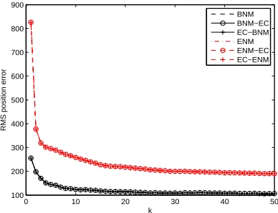
2.8 RMS position error comparison for example 3 with correct Q and ˆx0|0 = ¯x0.
Note that BNM, BNM-EC and EC-BNM essentially overlap with each other,
and ENM, ENM-EC and EC-ENM essentially overlap with each other. . . . 39
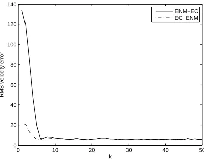
2.9 RMS velocity error comparison for example 3 with correct Q and ˆx0|0 = ¯x0.
Note that BNM, BNM-EC and EC-BNM essentially overlap with each other,
2.10 RMS position error comparison for example 3 with Q mismatch. Note that
BNM-EC essentially overlaps with EC-BNM, and ENM-EC essentially
over-laps with EC-ENM. . . 41
2.11 RMS velocity error comparison for example 3 with Q mismatch. Note that BNM-EC essentially overlaps with EC-BNM, and except for the small devia-tion at transient, ENM-EC essentially overlaps with EC-ENM. . . 42
2.12 RMS position error comparison for example 3 with mis-specified ˆx0|0. Note that BNM-EC essentially overlaps with EC-BNM, and ENM-EC essentially overlaps with EC-ENM. . . 43
2.13 RMS velocity error comparison for example 3 with mis-specified ˆx0|0. Note that BNM-EC essentially overlaps with EC-BNM, and except very little de-viation at transient, ENM-EC essentially overlaps with EC-ENM. . . 44
2.14 RMS position error comparison for example 4 . . . 45
2.15 RMS velocity error comparison for example 4 . . . 45
3.1 Comparison of estimate to the mean ofz in one run . . . 74
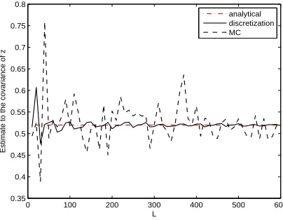
3.2 Comparison of estimate to the covariance ofz in one run . . . 74
3.3 Comparison of estimate to the mean ofz in another run . . . 75
3.4 Comparison of estimate to the covariance ofz in another run . . . 75
3.5 RMS error comparison for quantized estimation . . . 77
3.6 RMS position error comparison with correct Q and ˆx0|0 = ¯x0. Note that KF overlaps with IEC. . . 82
3.7 RMS velocity error comparison with correct Q and ˆx0|0 = ¯x0. Note that KF overlaps with IEC. . . 83
3.9 RMS velocity error comparison with Q mismatch. Note that KF and IEC-Q
have no noticeable difference. . . 85
3.10 RMS position error comparison with mis-specified ˆx0|0 . . . 85
3.11 RMS velocity error comparison with mis-specified ˆx0|0 . . . 86
3.12 RMS position error comparison for example 4 . . . 86
3.13 RMS velocity error comparison for example 4 . . . 87
5.1 RMS error comparison with pk = 0.8. Note that MMSE-a and MMSE-b overlap with each other. . . 140
5.2 RMS error comparison with pk = 0.5. Note that MMSE-a and MMSE-b overlap with each other. . . 141
5.3 RMS error comparison with pk = 0.2. Note that MMSE-a and MMSE-b overlap with each other. . . 142
5.4 RMS error comparison with p11= 1, p00 = 1 . . . 143
List of Tables
2.1 LMMSE estimators used in example 1 . . . 34
2.2 LMMSE estimators used in example 2 . . . 36
2.3 State estimators used in example 3 . . . 39
3.1 Comparison of computational burden . . . 77
3.2 Estimators used in inequality constrained estimation example . . . 82
3.3 Estimators used in noise-free measurement example . . . 84
5.1 Estimators used in Fig. 5.1 to Fig. 5.3 . . . 139
Chapter 1
Introduction
1.1 Background
The process of inferring the value of a quantity of interest from indirect, inaccurate and
uncertain observations is known as estimation [10]. More rigorously, estimation can be
viewed as the process of selection of a point from a continuous space—the “best estimate.”
The quantity of interest in an estimation problem can be a parameter—a time-invariant
quantity (parameter estimation), or the state of a dynamic system (state estimation).
Dynamic systems are encountered almost everywhere in reality, e.g., in target tracking,
chemical reaction, satellite guidance and navigation, power transmission and distribution,
orbit determination, weather and financial forecasting, optimal control, fault diagnosis. We
are interested to know the state of a dynamic system, but only indirect, inaccurate and
uncertain observations are usually available to us. So state estimation is extremely important
in practice.
In a typical state estimation problem, the estimator uses the knowledge about the
evolu-tion of the state (the system dynamics), the sensor (measurement system) and the
probabilis-tic characterization of the various random factors (uncertainties) and the prior information.
A celebrated solution to state estimation is the Kalman filter [62], which is optimal in the
is usually not valid. Next, depending on the applications, some of the extensions to the
classical state estimation will be briefly summarized. We describe these techniques following
largely [76].
In practice, either the system dynamics or measurement system can be nonlinear and
the driving noise may also be non-Gaussian. This leads to nonlinear filtering, which consists
of point estimation and density estimation [76]. The goal of point estimation is to get
some descriptive statistics of the random state, instead of its probability distribution. For
example, most point estimation approaches focus on getting the first two moments of the
state. Density estimation aims at estimating the probability distribution of the state.
To deal with the nonlinearity from system dynamics and/or measurement equations, in
nonlinear point estimation the simplest way is approximation by linearization. For example,
the most widely used Extended Kalman filter (EKF) successively linearizes around the latest
estimate through a first-order Taylor series expansion (TSE). The EKF is popular mainly
because of its simplicity, but its performance is not necessarily good. It is known that the
performance of EKF relies heavily on the degree of nonlinearity of the system dynamics
and/or measurement equations and the accuracy of the initial estimate [76]. From TSE,
we know that the linearization is an adequate approximation of its nonlinear counterpart
only when the latest estimate is sufficiently close to the quantity to be estimated, which can
rarely be guaranteed in practice. The error may build up over time and result in filtering
divergence. One compensation is to use iterated EKF (IEKF), in which the measurement
equation is repeatedly linearized around the most recent updated state estimate several times.
The IEKF usually outperforms the EKF somewhat, especially if the state update improves
state prediction greatly, but an improvement is not guaranteed in general [76]. Experience
indicates that after a couple of iterations the performance improvement diminishes. Another
second-order TSE and then applies the Kalman filter formulas for the gain calculation and
update. Its implementation is not as simple as the EKF. TSEs with orders higher than two
are rarely used in practice. Note that the EKF is derivative based, e.g., we need to calculate
Jacobian and even Hessian matrices, which requires differentiability of the nonlinear function.
In contrast, other nonlinear point estimation approaches introduced below are derivative free.
The idea of the EKF is to approximate a nonlinear function by its TSE approximation.
Another popular idea proposed in recent years is to use interpolation. Unlike the TSE
approximation which relies on the function value at only a single point, interpolation relies
on the function values at multiple points and it is possible to be derivative free [76]. There
are numerous interpolation formulas. Stirling’s is among the best. Under the Gaussian
assumption, the second-order Stirling interpolation based filter (DD2) [89] has fourth-order
error, compared with the order error of the EKF and third-order error of the
second-order EKF.
In contrast to the function approximation techniques [76], e.g., EKF, second-order EKF,
first-order Stirling interpolation based filter (DD1) [89] and DD2, that approximate the
in-volved nonlinear functions, moment matching techniques for nonlinear filtering approximate
the first two moments involved in the LMMSE filter directly [76]. Different moment matching
techniques differ from each other on the ways the first two moments involved in the LMMSE
filter are approximated. For example, the unscented transformation (UT), which is the key
to unscented filtering (UF) [60], approximates mean and covariance of a nonlinearly
trans-formed random vector by deterministically sampled sigma points and their corresponding
weights. The Gaussian filter [57] successively approximates each pdf by a moment-matching
Gaussian distribution and then uses Gauss-Hermite quadratures to compute the involved
first two moments.
Both TSE and Stirling’s interpolation approximate the involved nonlinear functions in a
linearization [76] approximates the original nonlinear stochastic system locally by a stochastic
model that is simple and linear in an optimal fashion so that linear filtering results can be
applied. While the EKF is not accurate if the estimation error is not small, the filter based on
stochastic linearization accounts for large errors within the expectations probabilistically and
thus tends to have a more conservative gain and better performance for the case involving
large estimation error. The main difficulty associated with stochastic linearization lies in
the (analytical or numerical) evaluation of the expectations. Statistical linearization [69]
approximates them by sample averages.
Density estimation is much harder than point estimation because the first two moments
are only two descriptive statistics of a distribution. In theory, density estimation can be
solved by Bayesian recursive filtering (BRF). The main difficulty for BRF comes from the
evaluation of the expectations of the transition density and likelihood function. Particle
filters [2] are sequential Monte-Carlo (SMC) simulation-based implementations of the BRF.
It approximates the posterior distribution by a random probability mass function (pmf).
The key to particle filtering is the choice of proposal distribution and resampling. As a
breakthrough in the SMC method, resampling was introduced to counteract degeneracy,
otherwise after several recursions weights of the random pmf will be concentrated at one
particle leaving negligible weights to the others [76]. Although particle filtering is a close
approximation to BRF, it achieves the significantly improved estimation performance at the
cost of a heavily increased computational burden.
State estimation plays a key role in target tracking. In contrast to other state estimation,
the challenges in target tracking are mainly from the measurement-origin uncertainty and
target motion uncertainty.
By measurement-origin uncertainty in target tracking, it is meant that the origin of a
also be from background clutter or countermeasures. In multiple-target tracking in
clut-ter, a measurement may or may not be from a specific target of interest. It may also be
from other targets or from background clutter or countermeasures. Most filters dealing with
measurement-origin uncertainty in target tracking follow the traditional two-stage strategy:
data association first and then estimate. That is, the origin of the measurements are
de-termined first and then measurement-origin known filtering techniques can be applied. For
instance, the nearest neighbor filter (NNF) [102,108] chooses the validated measurement that
is closest to the gate center and ignores the rest, then it treats the selected measurement as
if it were surely the true one and uses it to update the track. The NNF can be improved
significantly [76] by accounting for, in the estimation step, the probability that the NN
mea-surement is not really the true one if the validated meamea-surement set is not empty, leading to
the probabilistic nearest neighbor filter. The NNF only chooses the closest validated
mea-surement to the gate center and discards the rest. This is hard decision. A major drawback
is that the decision error (i.e., the closest validated measurement is not from the target) is
not taken into account in estimation. The probabilistic data association filter (PDAF) [12]
calculates the probability of each validated measurement to be from the true target and uses
them as weights to sum up all validated measurements (soft or no decision) as a whole to
up-date the track. The joint probabilistic data association filter (JPDAF) [48] is an extension of
the PDAF to track maintenance of multiple targets by following the same soft decision idea.
Three fundamental assumptions used by JPDAF [76] are that the established targets/tracks
are known, a validated measurement can have only one source, and at most one measurement
can originate from a target. Similar to the PDAF, the JPDAF calculates the probability of
each measurement to be from the established targets. Another popular method for
multiple-target tracking is multiple hypothesis tracking (MHT) [93], which differs from the JPDAF
in two fundamental aspects [76]: the associations are measurement-oriented, rather than
not just for the current time as in the JPDAF.
Another major difficulty in maneuvering target tracking is due to the target motion
uncertainty. In essence, maneuvering target tracking is a hybrid estimation problem in
which we need to estimate both the continuous target state and discrete target motion
mode [76]. Soft decision based multiple model (MM) approach, e.g., interacting multiple
model (IMM) [16], is becoming the mainstream in maneuvering target tracking [76], as
opposed to traditional hard decision based algorithms, e.g., variable dimension filter [5], and
input estimation algorithm [20]. The conventional hard decision based approaches have two
stages. They decide on a model first and then run a filter based on it as if it were the true
one. There is only one model chosen at each time and only the filter based on it is run
at any single time. The major drawback of the hard decision based approach is that the
decision errors with respect to the model are not accounted for in estimation [76]. The MM
approach assumes a set of models for the true mode, each having the possibility to be true
at the time. A bank of elemental filters, each based on a unique model in the set, is run.
The overall estimate is a weighted average of the results of elemental filters. In contrast to
the hard decision based approaches, all possible decisions and their error probabilities are
accounted for in the MM approach.
With the emerging of sensor networks, traditional state estimation problems are facing
new challenges. For example, the measurements are available from multiple sensors. How
to best utilize these multiple measurements is the key of estimation fusion [81]. There are
two basic fusion architectures. One is centralized fusion and the other is distributed
fu-sion, depending on whether the raw measurements are sent to the fusion center or not. In
centralized fusion, all raw measurements are sent to the fusion center, while in distributed
fusion, each sensor only sends in processed data. They have pros and cons in terms of
problem with distributed data. Distributed fusion is more challenging and has been a focal
point of most fusion research.
Other challenges faced by network-based state estimation include: due to unreliable
communication between local sensors and the processing center, packet transmission
de-lay [4,86,112,115,129] and multiple packet dropouts [98–100,113,114] are usually inevitable;
also, the constraints on communication bandwidth, power consumption [46, 70] and
com-putational capability should be considered, which make the distributed estimation [81] and
estimation problems with compressed [35, 128] or quantized data [33, 58] necessary; the
sen-sors often work asynchronously [1, 55, 56, 74, 82, 88, 122] instead of synchronously, which is
widely assumed in the literature; the sensors may also have different sampling rates and
communicate rates.
In reality, the evolution of the state may subject to constraints. For example, in ground
target tracking [65], the road networks can be described by equality or inequality constraints.
In the quaternion-based attitude estimation problem [15], the attitude vector must have a
unit norm. In a compartmental model with zero net inflow [27], mass is conserved. In an
undamped mechanical system, such as one with Hamiltonian dynamics, energy conservation
law holds. Likewise, in circuit analysis, Kirchhoff’s current and voltage laws hold. In a
chemical reaction, the species concentrations are nonnegative. All these make the constrained
state estimation necessary.
1.2 Research Objectives
As briefly summarized above, depending on applications, there are different extensions to the
classical state estimation. The main objective of this research is to deal with state estimation
with two types of unconventional measurements and two types of network-induced problems.
measurement considered is noise-free measurements and the other is set measurement. The
first type of network-induced problem is distributed estimation fusion with transformed data
and the second type is the one in the presence of multiple packet dropouts.
Conventionally, a measurement is assumed to be a point in the measurement space and
driven by noise. But in reality, for some applications, the measurements may be noise-free
or a subset of the measurement space. For example, state estimation problems under linear
or nonlinear equality constraints, with correlated or singular measurement noise can all be
formulated as those with noisy and noise-free measurements. State estimation problems
under linear or nonlinear inequality constraints, with quantized measurements can all be
formulated as those with point and set measurements. All these unconventional
measure-ments surely need special treatment in order to obtain the optimal or near optimal solutions
efficiently.
Considering the communication constraints, it is more beneficial for local sensors to
send in processed data with less communication in distributed estimation fusion. In terms
of estimation performance, it is better that the distributed estimation fusion with locally
processed data can achieve as close performance to the centralized fusion as possible and is
numerically more robust. The objective of research on this topic is to develop distributed
fusion algorithms which can achieve these desirabilities.
Due to unreliable communication between local sensors and the processing center, packet
dropouts may happen during transmission. The objective of research on this topic is to
propose LMMSE-optimal and MMSE-optimal estimators for state estimation in the presence
of packet dropouts.
1.3 Thesis Outline
Chapter 1 presents the background and objectives of this research work.
Chapter 2 deals with optimal state estimation with noisy and noise-free measurements.
Given only the first two moments and without any assumption on the rank of the
measure-ment matrix for noise-free measuremeasure-ment, it is pointed out that this estimation problem is in
essence just one with singular measurement noise and is not really a big deal in theory, with
the optimal solution provided by the batch LMMSE estimator. Two sequential forms of the
batch LMMSE estimator are obtained to reduce the computational complexity.
Chapter 3 addresses state estimation problems with point and set measurements. Inspired
by the estimation with quantized measurements developed by Curry [28], under a Gaussian
assumption, the MMSE state estimator with point measurements and set measurements of
any shape is proposed by discretizing continuous set measurements.
Chapter 4 discusses lossless linear transformation of sensor data for distributed estimation
fusion. By taking linear transformation of the raw measurements received by each sensor,
two optimal distributed fusion algorithms are proposed. Compared with existing fusion
algorithms, they have three nice properties.
Chapter 5 is about optimal state estimation in the presence of multiple packet dropouts.
An alternative form of LMMSE estimation in the presence of multiple packet dropouts is
proposed first. Then under a Gaussian assumption, the MMSE estimation is also proposed.
Chapter 6 draws conclusions from this research work and lists some future work to
Chapter 2
Optimal Linear State Estimation with Noisy
and Noise-free Measurements
2.1 Introduction and related research
As will be shown below, numerous state estimation problems can be formulated as those with
both noisy and noise-free measurements 1 (e.g., state estimation under linear or nonlinear
equality constraints, with correlated or singular measurement noise.)
For the case with noise-free measurements only, one simple heuristic [74,84] is to increase
the zero diagonal elements of the measurement noise covariance matrix artificially to a small
number, but optimality is lost and a stabilizing effect on the numerics of the Kalman filter
occurs. Another well established method is the so-called reduced-order filter [74,84], in which
a smaller dimensional state is used, as the name suggests. The key idea here is to express
the original state as a linear combination of the current measurement and the reduced-order
state from an invertible augmentation to the original measurement equation. In this way,
the possible numerical problem resulted from zero covariance matrices of the measurement
noises can be circumvented. But the computational complexity is not necessarily reduced
The state vectors of many dynamic systems evolve according to some linear or nonlinear
equality constraints. For example, in ground target tracking [65, 123, 125], if we treat roads
as curves without width, the road networks can then be described by equality constraints. In
the quaternion-based attitude estimation problem, the attitude vector must have a unit norm
[15]. In a compartmental model with zero net inflow [27], mass is conserved. In an undamped
mechanical systems, such as one with Hamiltonian dynamics, energy conservation law holds.
Likewise, in circuit analysis, Kirchhoff’s current and voltage laws hold. For state estimation
with noise-free measurements due to equality constraints, numerous results and methods are
available [51, 61, 66, 105, 116, 119, 124, 125, 131]. For example, the reparameterization method
simply reparameterizes the system model so that the equality constraints are not required
any more. It has several disadvantages. First, the physical meaning of the reparameterized
system state may vary and be different at different time instants. Second, the interpretation
of the reparameterized system state is less natural and more difficult [105]. Another popular
method for equality constrained estimation is the projection method [51, 61, 66, 105, 124,
125], in which the estimate is projected onto the constraint subspace. Unfortunately, it
has problems and limitations. Its main idea is to apply classical constrained optimization
techniques to the constrained estimation problem. Some other methods, e.g., maximum
probability method and mean square method, were also discussed in [105]. They are not free
of the limitations, either. Also, all existing work processes the noisy measurement first and
then the equality constraint. Is it the only choice or a good choice? If there are more than
one choice, how should the end user choose among them? Unfortunately, such questions
have not been answered in theory.
A white-noise observation model is widely used in target tracking. In practice, the
measurement noise may be colored [18, 19, 49, 50, 52, 77, 83, 95, 121]. A “brute force” solution
is to augment the state with measurement noise and thus the problem is reduced to a
a singular error covariance—an undesirable feature [11, 74]. To avoid this, the measurement
differencing approach was first proposed in [18].
Some but not all measurement components may be so accurate that it is occasionally
reasonable to assume that they are perfect, i.e., they have no error [17,19,44,45,47,54,59,83,
90,91]. This is of practical importance [47] since it is often the case, e.g., in many industrial
control systems [91]. For such a state estimation problem, the Kalman filter of a full system
order, with a possible numerically ill-conditioined gain matrix, is inappropriate [91]. In such
cases, reduced-order filters are preferable since there is no need to estimate those states
which are known exactly [54]. Actually to circumvent numerical problems, as discussed
below, Moore-Penrose pseudoinverse (MP inverse for short) can be simply used to replace
the inverse if the optimality criterion is LMMSE. Since the computational complexity of the
Kalman filter is mainly determined by the involved inverse, which has the same dimension as
the measurement, it should be noted that the computational complexity can not necessarily
be reduced by just reducing the order of the state.
As shown later, the state estimation problem with both noisy and noise-free
measure-ments is in essence just one with singular measurement noise and is not really a big deal
in theory. What matters is the computational complexity of the solution. So a main focus
of this chapter is to find computationally efficient ways and analyze their applicapability to
different scenarios.
This chapter is organized as follows. Sec. 2.2 formulates the problem. Sec. 2.3 gives some
cases with noise-free measurements so as to show our research work in this direction is useful.
Sec. 2.4 presents the batch LMMSE estimator. Sec. 2.5 presents two equivalent forms of
the sequential LMMSE estimator. Sec. 2.6 discusses extension to nonlinear measurements.
2.2 Problem formulation
Consider the following generic dynamic system
xk=Fk−1xk−1+Gk−1wk−1 (2.1)
with zero-mean white noise wk with cov(wk) =Qk ≥0 andxk ∈Rn,E[x0] = ¯x0, cov(x0) =
P0.
Assuming that two types of measurements of the system state are available at the same
time. The first type is noisy:
zk(1) =Hk(1)xk+vk(1) (2.2)
with zero-mean white noise vk(1) with cov(vk(1)) = Rk(1) > 0 and z(1)k ∈ Rm1. hw
ki, hvk(1)i and x0 are uncorrelated with each other.
The assumption R(1)k >0 is not restrictive in our framework, as explained in Sec. 2.3.4. The second type of measurement is noise free:
zk(2) =Hk(2)xk (2.3)
where zk(2) ∈Rm2.
One may think that z(2)k is always random since it is a measurement of the state. As shown later, this is not always true.
In this work, given only the first two moments, we try to obtain the LMMSE state
estimation with both noisy and noise-free measurements. That is,
ˆ
xLMMSEk|k =∆ E∗xk|zk
= arg min
ˆ
xk|k=ak+BkZk
where
zk ={z1,· · · , zk}, Zk = [z1′,· · · , zk′]′
zk = [(zk(1))′,(zk(2))′]′ (2.4)
MSE ˆxk|k
=E[(xk−xˆk|k)(xk−xˆk|k)′]
and ak, Bk do not depend on Zk.
2.3 Noise-free measurements
Before getting into details about how to obtain the optimal state estimation, let us discuss
some cases with both types of measurements to show that our work is not only meaningful
in theory but also useful for application.
2.3.1
Linear equality constraints
In this case, a linear equality constraint is placed on theestimand (quantity to be estimated):
Dxk =dk (2.5)
where matrix D and vectordk are both known.
Let
zk(2) =dk, Hk(2) =D
It can be easily seen that the above linear equality constraint is exactly a noise-free
measure-ment. So state estimation with linear equality constraints is a special case of the problem
tions were made in the derivation of their results. For example, except for [131], they all
made the Gaussian assumptions. Under the Gaussian assumption, the result in [119] was
claimed to be optimal in the sense of generalized maximum likelihood (GML) in which the
correlation between the pseudo measurement noise and the estimand was totally ignored;
the result in [116] and the maximum probability method in [105] were claimed to be optimal
in the sense of maximum a posterior probability (MAP); the mean square method in [105]
was claimed to be optimal in the sense of MMSE. Necessary conditions need to be
satis-fied by a constrained linear system, and one way to construct a homogeneously constrained
linear system based on the information of an unconstrained linear system was introduced
in [66]. [51,66] formulated the problem with the Gaussian assumption just to agree with the
assumptions in the standard Kalman filtering. [124] provided a geometric interpretation of
the results in [105], so the Gaussian assumption was maintained. Since our optimality
cri-terion is LMMSE, we only assume the first two moments to be known, which is the same as
in [131]. Another common assumption is that Dis of full row rank, otherwise, we can make
it full row rank by simply removing linearly dependent rows. But to obtain the rank of D
and find its linearly dependent rows may not be trivial. In addition, why is this assumption
needed? What is the advantage of it? This will be analyzed later. On the contrary, we do
not have any restrictions on the rank of Hk(2).
There was one common problem in the derivations of most existing results. The objective
functions are inconsistent before and after using linear constraints, although some of the
results are the same as a form of our sequential LMMSE filter. Specifically, the objective
function before using the linear constraints is MSE (in the average sense), while afterwards
it becomes fitting error in the least-squares sense, in which the estimate is treated as data.
2.3.2
Nonlinear equality constraints
In this case, a nonlinear equality constraint is placed on the estimand:
c(xk) = 0
where c(·) is some vector-valued nonlinear function.
Let
zk(2) = 0, h(2)k (xk) =c(xk)
Then state estimation with nonlinear equality constraints is a special case of the problem
with a nonlinear measurement model (see the section “extension to nonlinear measurements”
for details.)
This case has also been widely studied [61, 105, 119, 124, 125]. Under the Gaussian
as-sumption and linearization based on a first-order TSE, the result in [119] was claimed to be
approximately GML-optimal. [105] extended their state estimation results for linear equality
constraints to the case with nonlinear equality constraints. Under the Gaussian assumption,
a second-order TSE was utilized in [124, 125] to get better estimation results. [61] even put
constraints on the statistics of the distribution of the estimate and proposed a two-step
pro-jection method. The same problem and limitations mentioned in the above subsection exist
in these results.
2.3.3
Autocorrelated measurement noise
Suppose that only noisy measurements are available for the dynamic system (2.1) as follows
where the measurement noise hvki is autocorrelated instead of white:
vk+1 =Bkvk+vkw
with zero-mean white hvw
ki, uncorrelated with hwki and x0, and cov(vkw) =Rwk >0,
A “brute force” solution to the optimal state estimation problem in this case is as follows.
Let
xak =
x′
k vk′ ′
, Fka=
Fk 0
0 Bk
, Gak =
Gk 0
0 I
, wka=
w′
k (vkw)′ ′
Ha k =
Hk I
Then the above dynamic system can be rewritten as
xa
k=Fka−1xak−1+Gak−1wka−1
z(2)k =Hkaxak
As can be seen, the original noisy measurement zk(2) is now noise free with respect to (w.r.t.) the augmented statexa
k. As such, we only have noise-free measurements. As pointed
out in, e.g., [11, 18, 74], due to the increased state dimension and zero measurement noise,
numerical problems may arise if the inverse is still used as in the standard Kalman filtering,
which is undesirable. That is also why the “difference measurement” method [11, 74] is
popular for this case. But if the inverse is replaced by the MP inverse in the singular cases,
the optimal state estimation can still be obtained based on this augmented noise-free form.
Also, one bonus is that we will have the optimal estimate of the measurement noise at the
2.3.4
Singular measurement noise
Suppose that the measurement available for the dynamic system (2.1) is:
¯
zk = ¯Hkxk+ ¯vk (2.6)
where ¯Rk = cov(¯vk) with
R¯k = 0. We show that this case can be converted to our
formulation with both noisy and noise-free measurements.
It follows that
rank ¯Rk ∆
=m1 < m ∆
= dim (¯vk)
It then follows from singular value decomposition (SVD) that there must exist a unitary
matrix ¯Uk such that
¯
UkR¯kU¯k′ =
R(1)k 0m1×(m−m1) 0(m−m1)×m1 0(m−m1)×(m−m1)
where R(1)k >0 is an m1×m1 diagonal matrix. That is also why we can assumeR(1)k >0 in
our problem formulation without loss of generality.
Let
zk = ¯Ukz¯k
Then, Eq. (2.6) can be rewritten as
where
zk = [(zk(1))′,(z
(2)
k )′]′, Hk = [(Hk(1))′,(H
(2)
k )′]′ = ¯UkH¯k, vk = [(v(1)k )′,(v
(2)
k )′]′ = ¯Uk¯vk zk(1) ∈Rm1, z(2)
k ∈R
m2, H(1)
k ∈R
m1×n, H(2)
k ∈R
m2×n, v(1)
k ∈R
m1, v(2)
k ∈R m2
m2 =m−m1, cov(vk(1)) =R(1)k , cov(vk(1), vk(2)) = 0, vk(2) = 0 a.s.
Since ¯Uk is unitary and thus invertible, zk = ¯Ukz¯k is sufficient in the sense that the
LMMSE based on zk is equivalent to the LMMSE based on ¯zk. That is, the original noisy
measurements only Eq. (2.6) is equivalent to the following:
zk(1) =Hk(1)xk+vk(1) zk(2) =Hk(2)xk
which is exactly in the form of our formulation.
2.4 Batch LMMSE estimation
With the augmented zk in Eq. (2.4), the stacked measurement equation can be written as
zk =
Hk(1) Hk(2)
xk+
vk(1)
0m2×1
Define
Hk= [(Hk(1))′,(Hk(2))′]′ vk= [(vk(1))′,0′m2×1]
Then the equation becomes
zk =Hkxk+vk
where zk ∈ Rm1+m2, hvki is zero-mean white noise with cov(vk) = Rk = diag(Rk(1),0m2×m2) and uncorrelated withhwki and x0.
Given ˆxk−1|k−1 =E∗[xk−1|zk−1],Pk−1|k−1 = MSE(ˆxk−1|k−1) and zk, it is well known (see,
e.g., [73, 81]) that the batch LMMSE estimator of xk is:
Prediction:
ˆ
xk|k−1 =E∗[xk|zk−1] =Fk−1xˆk−1|k−1
Pk|k−1= MSE(ˆxk|k−1) =Fk−1Pk−1|k−1Fk′−1+Gk−1Qk−1G′k−1
Update:
ˆ
xk|k =E∗[xk|zk−1, zk] = ˆxk|k−1+Pk|k−1Hk′Sk+(zk−Hkxˆk|k−1)
Pk|k = MSE(ˆxk|k) =Pk|k−1−Pk|k−1Hk′Sk+HkPk|k−1
Sk =HkPk|k−1Hk′ +Rk
In this dissertation, A+ stands for the unique MP inverse of matrix A. It reduces to A−1
whenever A−1 exists.
Compared with the standard Kalman filtering, nothing is different except that the inverse,
if not exist, is now replaced by the MP inverse.
Since Rk ≥ 0 in general, the batch LMMSE estimator with both noisy and noise-free
measurements needs to calculate the MP inverse Sk+, which is (m1+m2)×(m1+m2).
Even if x0, wk and vk(1) all have a Gaussian distribution with a nonsingular covariance
ofxk is nonexistent and the MAP estimate ofxkdoes not exist if Pk|kis not positive definite.
That is also one of the reasons why we choose LMMSE as our optimality criterion.
2.5 Sequential LMMSE estimation
To reduce the computational complexity of the batch LMMSE estimator, we obtain two
equivalent sequential forms of the LMMSE estimator. They process the noisy and noise-free
measurements sequentially and thus have reduced computation.
2.5.1
Form 1
Theorem 1 (Sequential LMMSE, form 1). Given ˆxk−1|k−1 =E∗[xk−1|zk−1],Pk−1|k−1 =
MSE(ˆxk−1|k−1) and zk, one form of the sequential LMMSE estimator ofxk is:
Prediction: Same as in the batch LMMSE estimator.
Update by the noisy measurement:
ˆ
x(1)k|k = ˆxk|k−1+Pk|k−1(Hk(1))′(S
(1)
k )−1(z
(1)
k −H
(1)
k xˆk|k−1) (2.7)
Pk(1)|k =Pk|k−1−Pk|k−1(Hk(1))′(S
(1)
k )−
1H(1)
k Pk|k−1
Sk(1) =Hk(1)Pk|k−1(Hk(1))′+R
(1)
k (2.8)
Update by the noise-free measurement:
ˆ
xk|k= ˆx(1)k|k+Pk(1)|k(Hk(2))′(S
(2)
k )+(z
(2)
k −H
(2)
k xˆ
(1)
k|k) (2.9)
Pk|k=Pk(1)|k −Pk(1)|k(Hk(2))′(S
(2)
k )+H
(2)
k P
(1)
k|k (2.10)
Sk(2) =Hk(2)Pk(1)|k(Hk(2))′ (2.11)
E∗[x
k|zk−1, z(1)k ] and P
(1)
k|k = MSE(ˆx
(1)
k|k).
Since the LMMSE estimator E∗[x
k|zk−1, zk] always has the quasi-recursive form [73]:
ˆ
xk|k =E∗[xk|zk−1, zk] =E∗[xk|zk−1, zk(1), z
(2)
k ] = ˆx
(1)
k|k+C1,2C
+ ˜
z∗ 2|1z˜
∗
2|1
where
˜
z∗2|1 =z(2)k −E∗[zk(2)|zk−1, zk(1)] =zk(2)−Hk(2)xˆ(1)k|k=Hk(2)(xk−xˆ(1)k|k) Cz˜∗
2|1 = cov(˜z
∗
2|1) =H (2)
k P
(1)
k|k(H
(2)
k )′
∆
=Sk(2) C1,2 = cov(˜x(1)k|k,z˜∗2|1) =P
(1)
k|k(H
(2)
k )′
(2.9) follows. Also,
Pk|k = MSE ˆxk|k
=Pk(1)|k−C1,2Cz˜+∗ 2|1C
′
1,2 =P (1)
k|k −P
(1)
k|k(H
(2)
k )′(S
(2)
k )+H
(2)
k P
(1)
k|k
Remark: This sequential LMMSE estimator needs to calculate anm1×m1 inverse (Sk(1))−1
and anm2×m2 MP inverse (Sk(2))+. This is less demanding than computing the (m1+m2)×
(m1+m2) MP inverse Sk+ in the batch LMMSE estimator.
Remark: IfPk(1)|k >0 andHk(2) is of full row rank, then (Sk(2))+ can be replaced by (S(2)
k )−1
and this sequential LMMSE estimator will be exactly the same as the one in [105] for a linear
equality constrained state estimation problem. But there is still a significant difference. This
sequential LMMSE estimator is free of the problem and limitations of the existing results
discussed above.
LMMSE estimator of xk was presented in [131]:
ˆ
xk|k = (I −Jk)ˆxk(1)|k+Jk(Hk(2))+z
(2)
k (2.12)
where
Jk =Pk(1)|k(Hk(2))′(Sk(2))+Hk(2)
This can also be easily proved from our sequential LMMSE estimator sinceHk(2)(Hk(2))+ =I.
This weighted average form does provide a better understanding of the mathematical
mean-ing behind ˆxk|k, which is a weighted average of ˆx(1)k|k and (Hk(2))+z
(2)
k (a particular solution to
the linear equality constraint equation (2.5)). But computationally, this form is not preferred
for two reasons. First, it requires two MP inverses: (Hk(2))+ = (H(2)
k )′(H
(2)
k (H
(2)
k )′)−1 and
(Sk(2))+. Our sequential LMMSE estimator only needs (S(2)
k )+. Second, it is valid only when Hk(2) is of full row rank, but our sequential LMMSE estimator does not have this limitation.
2.5.2
Form 2
Theorem 2 (Sequential LMMSE, form 2). Given ˆxk−1|k−1 =E∗[xk−1|zk−1],Pk−1|k−1 =
MSE(ˆxk−1|k−1) and zk, an alternative form of the sequential LMMSE estimator ofxk is:
Prediction: Same as in the batch LMMSE estimator.
Update by the noise-free measurement:
ˆ
x(2)k|k=E∗[xk|zk−1, zk(2)] = ˆxk|k−1+Pk|k−1(Hk(2))′(S
(2)
k )
+(z(2)
k −H
(2)
k xˆk|k−1)
Pk(2)|k = MSE(ˆx(2)k|k) =Pk|k−1−Pk|k−1(Hk(2))′(S
(2)
k )+H
(2)
k Pk|k−1
Update by the noisy measurement:
ˆ
xk|k= ˆx(2)k|k+Pk(2)|k(Hk(1))′(S
(1)
k )−1(z
(1)
k −H
(1)
k xˆ
(2)
k|k)
Pk|k=Pk(2)|k−Pk(2)|k(Hk(1))′(Sk(1))−1Hk(1)Pk(2)|k Sk(1) =Hk(1)Pk(2)|k(Hk(1))′+R(1)k
Proof: Parallel to that of Theorem 1.
Remark: If the noise-free measurement is due to some linear equality constraint (2.5),
this form is contrary to the common practice of processing the constraints later.
Remark: Form 1 and form 2 have the same computational complexity.
Remark: If Hk(2) is of full row rank, then a nice equivalent weighted average form of ˆx(2)k|k
is
ˆ
x(2)k|k = (I−Lk)ˆxk|k−1+Lk(Hk(2))+z
(2)
k
where
Lk =Pk|k−1(Hk(2))′(S
(2)
k )+H
(2)
k
which can be easily proved from form 2 using Hk(2)(Hk(2))+ = I. The same remarks as for
form 1 can be made here.
Remark: Since both forms of the sequential LMMSE estimator are equivalent to the batch
LMMSE estimator, both forms have exactly the same performance. Then, the processing
order for zk(1) and z(2)k does not matter in either performance or computation.
If the noise-free measurement is from a linear equality constraint (2.3) and the estimator
is initialized by ¯x0 and P0, the following theorem shows that the LMMSE update by the
noise-free measurement in both of the sequential forms can be simply skipped without a
Theorem 3. If the noise-free measurement is from a linear equality constraint (2.3) and
ˆ
x0|0 = ¯x0, P0|0 =P0, then for sequential LMMSE estimator form 1, we have
ˆ
xk|k= ˆx(1)k|k, Pk|k=Pk(1)|k
and for sequential LMMSE estimator form 2, we have
ˆ
x(2)k|k = ˆxk|k−1, Pk(2)|k =Pk|k−1
Proof: In this case, z(2)k is known deterministically. If ˆx0|0 = ¯x0, P0|0 = P0, it then
follows from (2.3) that for form 1
z(2)k =E∗[zk(2)|zk−1, z(1)k ] =Hk(2)xˆ(1)k|k
and for form 2
zk(2) =E∗[zk(2)|zk−1] =Hk(2)xˆk|k−1
The theorem can then be easily shown.
Remark: This result for constrained state estimation agrees with Theorem 2 in [132]
which dealt with constrained least-squares parameter estimation.
Remark: If the noise-free measurement is from a linear equality constraint, then ¯x0 and
P0 can not be designated arbitrarily and should satisfy some necessary conditions, as pointed
out in [66].
Remark: It should be noted that Theorem 3 is obtained under the assumption that the
constrained LMMSE estimation can be obtained optimally. In practice, this optimality can
not be guaranteed due to model mismatch (e.g., in target tracking) or nonlinearity in the
estimation performance. Note also that if the noise-free measurement is random, Theorem
3 does not hold in general. Numerical examples to show these points are provided later.
If the noise-free measurement is from a linear equality constraint, then we need to double
check whether the estimate really satisfies the constraint. The following theorem shows that
all estimates really do so.
Theorem 4. For estimates from all forms, we have
Hk(2)xˆk|k−1 =zk(2), H
(2)
k xˆk|k=zk(2), H
(2)
k xˆ
(1)
k|k =z
(2)
k , H
(2)
k xˆ
(2)
k|k =z
(2)
k
Proof: Since the batch and sequential LMMSE estimators are equivalent, only sequential
form 1 is used to show that Hk(2)xˆk|k =z(2)k for simplicity.
It follows from Eq. (2.9) that
zk(2)−Hk(2)xˆk|k = (I −Sk(2)(S
(2)
k )+)H
(2)
k (xk−xˆ(1)k|k)
and thus, by the unbiasedness of ˆx(1)k|k,
E[zk(2)−Hk(2)xˆk|k] = 0
and
cov(zk(2)−Hk(2)xˆk|k) = (I−S
(2)
k (S
(2)
k )
+)S(2)
k (I−(S
(2)
k )
+S(2)
k ) = 0
Sozk(2) =Hk(2)xˆk|k almost surely.
Hk(2)xˆ(2)k|k=zk(2) can be proved similarly. Hk(2)xˆ(1)k|k=zk(2) and Hk(2)xˆk|k−1 =zk(2) then follow
from Theorem 3.
Remark: Hk(2)xˆk|k=zk(2) and H
(2)
k xˆ
(2)
k|k =z
(2)
constraint).
Since ˆxk|k is the LMMSE estimate of xk given zk and Pk|k is the corresponding MSE
matrix, they have the following properties:
• Pk|k ≤ Pk(1)|k ≤ Pk|k−1 in general. But if the noise-free measurement is from a linear
equality constraint and ˆx0|0 = ¯x0, P0|0 =P0, we have Pk|k =Pk(1)|k.
• Pk|k ≤ Pk(2)|k ≤ Pk|k−1 in general. But if the noise-free measurement is from a linear
equality constraint and ˆx0|0 = ¯x0, P0|0 =P0, we have Pk(2)|k =Pk|k−1.
• Ifx0,wk and vk(1) are jointly Gaussian distributed, ˆxk|k andPk|k are also optimal in the
sense of MMSE.
2.6 Extension to nonlinear measurement
Although the batch LMMSE estimator is optimal, due to its heavier computational burden,
it is not preferred. If the computational burden is concerned, the sequential forms are
preferred.
Both sequential forms are equivalent to the batch LMMSE estimator and have the same
computational complexity. Since form 1 is already simple enough, what is the specific reason
or advantage to adopt and derive form 2? What is the benefit to have these two forms? How
should the user choose between them? There should be no preference between these two
forms if only linear measurements are involved. But if one or both of zk(1) and zk(2) are nonlinear, there is a preference. That is, with linear measurements only, the performance
is independent of the processing order of zk(1) and zk(2). With nonlinear measurements, the order matters.
As demonstrated in [31, 41], for nonlinear filtering, sequential processing can not only
when the less nonlinear measurement is processed first, prediction and update by the more
nonlinear measurement will have a better reference point for function approximation based
nonlinear filters [78] (e.g., EKF and DD2 [89]) and sigma points or quadrature points for
moment approximation based nonlinear filters [78] (e.g., UF [60] and Gaussian Hermite filter
(GHF) [57]). This will be used as guideline for sequential processing in nonlinear filtering.
2.6.1
Nonlinear noisy measurement
In this case, the noisy measurement is nonlinear
zk(1) =h(1)k (xk, vk(1)) (2.13)
while the noise-free measurement is still linear.
Since the noise-free measurement is linear, we should use it first for update. The update
ˆ
x(2)k|k andPk(2)|k by using the noise-free measurement will be optimal. Then prediction and the update by using the noisy measurement should have better accuracy than if the noise-free
measurement is used after the noisy one.
In each cycle, prediction and the update by noise-free measurement are exactly the same
as in Theorem 2, and the update by noisy measurement can be done as follows:
ˆ
xk|k = ˆx(2)k|k+C2,1Cz˜+∗ 1|2z˜
∗
1|2 (2.14)
Pk|k =Pk(2)|k−C2,1Cz˜+∗ 1|2C
′
2,1 (2.15)
˜
z∗
1|2 =z (1)
k −E∗[z
(1)
k |zk−1, z
(2)
k ] (2.16)
Cz˜∗
1|2 = cov(˜z
∗
1|2) (2.17)
2.6.2
Nonlinear noise-free measurement
In this case, the noisy measurement is still linear while the noise-free measurement is
non-linear:
zk(2) =h(2)k (xk) (2.19)
For the same reason as in the above subsection, we should update by the noisy
measure-ment first, and then the noise-free measuremeasure-ment.
In each cycle, prediction and sequential update steps are the same as in the above
sub-section with z(1)k and z(2)k interchanged.
Remark: If the noise-free measurement is from a nonlinear equality constraint and the
LMMSE estimator is initialized by ˆx0|0 = ¯x0, P0|0 =P0, it can be easily shown as in Theorem
3 that the update by the noise-free measurement can be skipped.
2.6.3
Nonlinear noisy and noise-free measurements
In this case, both the noisy measurement (2.13) and the noise-free measurement (2.19) are
nonlinear.
In this case, we need to first measure the nonlinearity of h(1)k (·) and h(2)k (·). If h(kj)(·) is less nonlinear than h(ki)(·), i, j = 1,2, i 6= j, we can use the following general equations to obtain the sequential LMMSE estimator.
update byzk(j) can be done as:
ˆ
x(kj|)k=E∗[xk|zk−1, zk(j)] = ˆxk|k−1+Cx˜k|k−1˜zj∗C
+ ˜
z∗
jz˜ ∗
j
Pk(|jk)=Pk|k−1−Cx˜k|k−1z˜∗jC
+ ˜ z∗ jC ′ ˜
xk|k−1z˜∗j
˜
z∗
j =z
(j)
k −E∗[z
(j)
k |zk−1] Cz˜∗
j = cov(˜z ∗
j), Cx˜k|k−1z˜∗j = cov(˜xk|k−1,z˜ ∗
j)
The update by zk(i) can be done as (2.14) through (2.18) with zk(1) replaced by zk(j) and zk(2)
replaced by z(ki).
Remark: Due to the nonlinearity of zk(i) or zk(j) or both, we do not have an elegant analytical form for E∗[z(j)
k |zk−1], E∗[z
(i)
k |zk−1, z
(j)
k ], Cz˜∗
j, Cz˜i∗|j, C˜xk|k−1z˜
∗
j and Cj,i in general,
but they can be approximated by EKF, UF, DD2, GHF and even from the original definition
of LMMSE estimation, as in [130].
Remark: If the above extension to nonlinear measurements is used to handle constrained
estimation problem, then one natural theoretical question is whether the final estimate
sat-isfies the given constraints. It should be noted that the optimality criterion used in this
work is LMMSE conditioned on all measurement information up to the current time. Since
the equality constraints are already included in the conditioning, ˆxk|k and Pk|k should have
achieved this goal approximately. If ˆxk|k satisfies the equality constraints (e.g., when ˆxk|k
and Pk|k are obtained precisely without any approximation), then it is what we are looking
for, otherwise we have to make a choice between the LMMSE optimality criterion and the
equality constraints. If the criterion is chosen, then ˆxk|k is what we are looking for, otherwise
2.7 Illustrative examples
By Theorem 3, if the noise-free measurements are from equality constraints, then under
certain conditions, the update by the equality constraints is redundant. We also pointed out
that if there exists model mismatch or nonlinearity or ifzk(2) is random, two-step update will improve performance in general. In the following, we further verify these findings through
numerical examples.
Consider the following dynamic system, which describes the motion of an on-road vehicle
[66]:
xk=Fk−1xk−1+Gk−1uk−1+wk−1
where
xk = [ xk yk ˙xk ˙yk ]′, wk ∼ N(0, Qk), x0 ∼ N(¯x0, P0), P0 =NkP0uNk
Fk =
1 0 T 0
0 1 0 T
0 0 1 0
0 0 0 1
, Gk= 0 0
T sinθ
T cosθ
, Qk =
30 10√3 0 0
10√3 10 0 0
0 0 10 10√3/3
0 0 10√3/3 10/3
Nk =I4−(Hk(2))′(H
(2)
k (H
(2)
k )′)−
1H(2)
k , H
(2)
k = [ 0 0 1 −tanθ ]
θ =π/3, T = 2, uk =
1, ifk is odd
−1, ifk is even
¯
x0 and P0u will be given later. The state satisfies the following linear equality constraint [66]
Hk(2)xk = 0 (2.20)
width) is θ.
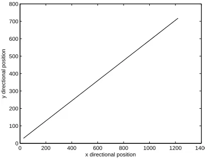
Figs. 2.1 and 2.2 show the true vehicle trajectory and velocity in one run in the
two-dimensional Cartesian coordinate plane. It can be seen that the given linear equality
con-straint is satisfied.
0 200 400 600 800 1000 1200 1400 0
100 200 300 400 500 600 700 800
x directional position
y directional position
Figure 2.1: Vehicle trajectory in one run
−15 −10 −5 0 5 10 15 20 25 30 −10
−5 0 5 10 15 20
x directional velocity
y directional velocity
Figure 2.2: Vehicle velocity in one run
We want to estimate the state in the LMMSE sense based on the measurements and
Qk:
Qmisk =
30 10√3 0 0
10√3 10 0 0
0 0 13.25 0.1443
0 0 0.1443 13.0833
is used in place ofQk in some estimators, possibly along with a mis-specified initial estimate
ˆ
xmis0|0 = ¯x0+ [ 0m 0m 6m/s 12m/s ]′
Also, all results were averaged over 200 Monte Carlo runs.
2.7.1
Example 1
In this example, the measurement provided by one type of sensor is described by
zk(1) =Hk(1)xk+vk(1) zk(3) =Hk(3)xk
where
vk(1) ∼ N(0, Rk(1)), Hk(1) =
1 0 0 0
0 1 0 0
, H
(3)
k = [ 2 3 0 0 ], R
(1)
k = diag{400m
2,400m2
}
That is,z(3)k is a perfect measurement, which is random. It is also known that
¯
x0 = [ 0m 0m 10√3m/s 10m/s ]′, P0u = diag(400m2,400m2,10(m/s)2,10(m/s)2)
which use the true Qk and are initialized with ˆx0|0 = ¯x0.
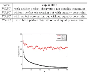
Table 2.1: LMMSE estimators used in example 1
name explanation
P OEC with neither perfect observation nor equality constraint
P OEC without perfect observation but with equality constraint
P OEC with perfect observation but without equality constraint
P OEC with both perfect observation and equality constraint
0 10 20 30 40 50
5 10 15 20 25
k
RMS position error
P OEC P OEC P OEC P OEC
Figure 2.3: RMS position error comparison for example 1. Note that P OEC overlaps with
P OEC and P OEC overlaps with P OEC.
As is clear from the simulation results, on the one hand, the update by the equality
constraint is really unnecessary—it does not improve performance. On the other hand, the
update by the perfect observations is indispensable—it leads to a significant performance
improvement. It should be noted that under our problem formulation, both the perfect
0 10 20 30 40 50 3.5 4 4.5 5 5.5 6 6.5 7 7.5 8 k
RMS velocity error
P OEC P OEC P OEC P OEC
Figure 2.4: RMS velocity error comparison for example 1. Note that P OEC overlaps with
P OEC and P OEC overlaps with P OEC.
2.7.2
Example 2
In this example from [66], the measurement provided by another type of sensor is described
by
zk(1) =Hk(1)xk+vk(1)
where
vk(1) ∼ N(0, R(1)k ), Hk(1) =
1 0 0 0
0 1 0 0
0 0 0 1
, R(1)k = diag(400m2,400m2,10(m/s)2)
It is also known that
¯
x0 = [ 0m 0m 10√3m/s 10m/s ]′, P0u = diag(400m2,400m2,10(m/s)2,10(m/s)2)
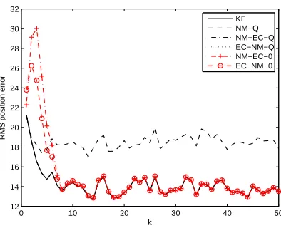
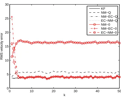
Figs. 2.5, 2.6 and 2.7 show comparison results of LMMSE estimators in Table 2.2.
Checking against the condition stated in Theorem 3, it can be easily justified that the