Input-to-state stability for discrete-time time-varying
systems with applications to robust stabilization of systems in
power form
Dina Shona Laila
1,2and Alessandro Astolfi
1Abstract
Input-to-state stability (ISS) of a parameterized family of discrete-time time-varying nonlinear systems is investigated. A converse Lyapunov theorem for such systems is developed. We consider parameterized families of discrete-time systems and concentrate on a semiglobal practical type of stability that naturally arises when an approximate discrete-time model is used to design a controller for a sampled-data system. An application of our main result to time-varying periodic systems is presented, and this is used to solve a robust stabilization problem, namely to design a control law for systems in power form yielding semiglobal practical ISS (SP-ISS).
Key words: Converse Lyapunov theorem; Discrete-time system; Input-to-state stability; Nonholonomic systems; Nonlinear systems; Power forms; Time-varying system.
1 Introduction
The prevalence of computer controlled systems and the fact that nonlinearities that arise naturally in most plants dynamics often can not be neglected in controller design, have driven people to study and investigate non-linear sampled-data control systems. A framework for discrete-time control design via approximate models of the plant has been proposed in [19]. Within this frame-work, a parameterized family of discrete-time models of the plant is used to perform the controller design, aim-ing at stabilizaim-ing the original continuous-time plant. As indicated in [19], time-invariant models that are usually used in design are often inadequate in practice. There is a class of controllable nonlinear systems that may not be stabilizable using time-invariant control, but there exist time-varying controls to stabilize such systems [2, 26]. Since there are many systems in applications that belong to this class, the stabilization problem using time-varying control has become an important topic of study. In [22], a systematic design of time-varying controllers for a class of controllable systems without drift has been proposed. Stabilization using sinusoids for nonholonomic systems in power form was studied in [31]. A number of more recent works were based on
1
The authors are with the Electrical and Electronic En-gineering Department, Imperial College London, Exhibition Road, London SW7 2AZ, UK.
2
Corresponding author. Tel:+44-20-75946108, Fax:+44-20-75946282, E-mail:{d.laila, a.astolfi}@imperial.ac.uk.
these early results, e.g. [4] that studied exponential sta-bilization using Lyapunov approach, and [12] in which exponential stabilization for homogeneous systems was thoroughly investigated.
Among the results that are available in the literature, there are only few that consider input-to-state stabiliza-tion using time-varying control. Input-to-state stability (ISS) is a type of robust stability for nonlinear systems with inputs (see [25, 27]). Indeed, ISS is very impor-tant, especially when dealing with systems in the pres-ence of disturbances. The first papers presenting Lya-punov characterization of ISS for time-varying nonlin-ear systems are [3, 8]. More recently, the authors of [18] have studied the problem using averaging technique. All the aforementioned works consider continuous-time sys-tems. To the best of the authors knowledge, the only re-sults on discrete-time systems are given in [6, 17], where asymptotic stability for discrete-time time-varying sys-tems is studied. In [5], the same authors have used the results of [6] to prove a converse Lyapunov theorem for ISS for discrete-time time-invariant systems.
(SP-ISS). Our main result is a converse Lyapunov theorem that can be seen as a discrete-time counterpart of the result of [3], and at the same time as a generalization of the results of [5,6]. We also present an application of our main result to time-varying periodic systems.
Moreover, to illustrate the applicability of the main re-sults, we address a robust stability design for a sub-class of driftless control systems, which have a special structure calledpower form. We opted to focus on the sampled-data stabilization of this class of systems to achieve SP-ISS of the closed-loop system, for the follow-ing reasons. First, we can find a simple (strict) SP-ISS Lyapunov function for this class of systems, and second, because of the prevalence of using discrete-time con-trollers in real life applications. Systems in power form are commonly used to model the kinematic equations of
nonholonomicsystems such as mobile robots. Due to the
functionalities of mobile robots, it is preferable to use a digital computer to steer and drive such systems, as the device requires much less space and it can handle other tasks simultaneously, such as data collection, while it is controlling the position of the robots. Since a mobile robot is a mechanical - therefore analog - plant, designing a digital controller for this system is a sampled-data con-trol design problem. Considering the semiglobal practi-cal property also makes sense, since we may assume that in practice the state space for the system is bounded.
The paper is organized as follows. In Section 2, we present preliminaries where notation and definitions are introduced. The main result is presented in Section 3. Section 4 is dedicated to an application of the main result to SP-ISS design problem for systems in power form. Design examples are presented in Section 5, and we conclude in Section 6.
2 Preliminaries
2.1 Definitions and notation
The set of real and natural numbers (including 0) are denoted respectively byRandN. A functionγ:R≥0→ R≥0 is of classK if it is continuous, strictly increasing
and zero at zero. It is of classK∞ if it is of classKand unbounded. Functions of classK∞are invertible. A con-tinuous functionβ:R≥0×R≥0→R≥0is of class-KLif
β(·, τ) is of class-Kfor eachτ ≥0 andβ(s,·) is decreas-ing to zero for eachs >0. Given two functionsα(·) and
γ(·), we denote their composition and multiplication as
α◦γ(·) andα(·)×γ(·), respectively.
To begin with, we consider nonlinear time-varying sys-tems described by
˙
x=f(t, x(t), d(t)), (1)
wherex∈Rnandd∈Rmare the states and exogenous
disturbances, respectively. Assume that the system (1) is between a sampler and zero order hold. The
parame-terized family of discrete-time model of (1) is written as
x(k+ 1) =FT(k, x(k), d(k)), (2)
where the free parameter T > 0 is the sampling pe-riod. Assume that the functionf is locally Lipschitz and
f(t,0,0) = 0. Without loss of generality we may assume the same conditions forFT. For any exogenous distur-banced: N→Rm, we denote kdk∞ := supk∈Nkd(k)k.
We use the notation UB¯, for the set of disturbances d
such that kdk∞ ≤ 1. We denote x◦ := x(k◦),k◦ ≥ 0, and Id the identity function, i.e. Id(s) = s. For any functions or variablesh we use the simplified notation
h(k,·) :=h(kT,·).
We emphasize that for nonlinear systems the exact discrete-time model Fe
T(k, x(k), d(k)) is usually not
known, since it requires solving a nonlinear initial value problem which is almost impossible in general (see [16] for more details). Although for some classes of non-linear systems with special structure it is possible to compute explicitly the exact discrete-time model, the discretization usually destroys the special structure of the systems, which left the discrete-time model not useful for design purposes. Moreover, for systems with disturbances, the exact discrete-time model may not be computable anymore (see Section 5.2 for example). For these reasons, throughout the paper we assume that (2) is obtained by approximating the exact discrete-time model of (1). To guarantee that (2) is a good approxi-mation of (1), we assume thatFT satisfies the following consistency property that is used to limit the mismatch.
Definition 2.1 (One-step consistency) [16] The
fa-mily of approximate discrete-time modelsFT is said to be
one-step consistent with the exact discrete-time models
Fe
T if given any strictly positive real numbers ∆x,∆d,
there exist a function%∈ K∞andT∗>0such that
|Fe
T −FT| ≤T %(T), (3)
for allk≥k◦,T ∈(0, T∗),|x◦| ≤∆xandkdk∞≤∆d.
One-step consistency is commonly used in numerical analysis literature (see for instance [7, 16, 20, 30]). Al-though Fe
T is not known, the consistency property is
checkable [16]. Moreover, since we consider a semiglobal property, we assume that Fe
T and FT are globally
de-fined. We will use the following definitions and techni-calities to construct and prove our main results. Note that the following definitions are modifications of those given in [5, 6].
Definition 2.2 (Semiglobal practical ISS) The fa-mily of systems (2) is semiglobally practically
input-to-state stable (SP-ISS) if there existβ ∈ KLandγ ∈ K,
such that for any strictly positive real numbers∆x,∆d, δ
there existsT∗>0such that the solutions of the system
satisfy
for allk≥k◦,T ∈(0, T∗),|x◦| ≤∆x, andkdk∞≤∆d.
Moreover, if there is no disturbance (d= 0), the system is
semiglobally practically asymptotically stable (SP-AS).
Definition 2.3 (SP-ISS Lyapunov function) A
fa-mily of functionsVT :R×Rn→R≥0is a family of
SP-ISS Lyapunov functions for the family of systems (2) if
there exist functionsα,α∈ K∞, a positive definite
func-tionαand a functionχ∈ K, and for any strictly positive
real numbers∆x,∆d, ν1, ν2, δthere exists strictly positive
numbersT∗andL, such that
α(|x|)≤VT(k, x)≤α(|x|), (5) |x| ≥χ(|d|)+ν1 ⇒
VT(k+ 1, FT)−VT(k, x)≤ −T α(|x|), (6)
VT(k+ 1, FT)≤VT(k, x) +ν2, (7)
for allk≥k◦, T ∈(0, T∗),|x| ≤∆x, andkdk∞ ≤∆d,
and |VT(k, x
1)−VT(k, x2)| ≤L|x1−x2| , (8)
for allk≥k◦,T ∈(0, T∗)andxi ∈[δ,∆x], i={1,2}.
Moreover, ifd= 0, the family of functionsVT is called a
family of SP-AS Lyapunov functions andVT is called a
smooth Lyapunov function if it is smooth inx∈Rn.
Consider nonlinear time-varying systems with control input: x˙ =f(t, x(t), u(t), d(t)), (9)
whereu∈Rlis a feedback controlu(t) :=u(x(t)). The
parameterized family of discrete-time model of (9) is
x(k+ 1) =FT(k, x(k), u(k), d(k)). (10)
We use the following assumption forFT in (10).
Assumption 2.1 There exists T∗ > 0 sufficiently
small, such that for allT ∈(0, T∗), and allk≥k
◦, FT
is continuous and
limT→0FT(k+ 1, x(k), u(k), d(k))→x(k).
Note that the continuity assumption ofFT does not nec-essarily require continuity of the control signalu(k). If we use the approximate model (10) to design a discrete-time controller, we can obtain a discrete-discrete-time controller
u(k) :=uT(x(k)) that is parameterized by T.
Definition 2.4 LetT >ˆ 0 be given and for each T ∈
(0,Tˆ)let the functionsVT :R×Rn→R
≥0anduT :R×
Rn →Rmbe defined. The pair(uT, VT)is a semiglobally
practically input-to-state stabilizing (SP-ISS) pair for the
system (10) if there exist functionsα,α∈ K∞, a positive
definite functionαand a functionχ∈ Ksuch that for any
strictly positive real numbers ∆x,∆d, ν1, ν2 there exist
strictly positive real numbersM andT∗, withT∗ ≤ Tˆ,
such that (5), (6), (7), (8) and
|uT(k, x)| ≤M , (11)
hold, for allk≥k◦,T ∈(0, T∗),|x| ≤∆x, andkdk∞≤
∆d. Moreover, ifd= 0, the pair(VT, uT)is called a
SP-AS pair.
Remark 2.1 While due to continuity of solutions con-dition (7) is not needed in the continuous-time context, we require this condition to guarantee boundedness of trajectories (see [19] for more details).
Definition 2.5 (∆-UBIBS) The family of systems (2)
is∆- uniformly bounded input bounded state (∆-UBIBS)
if there exist functions σ1, σ2 ∈ K, and for any strictly
positive real numbers ∆x,∆d, νb, δb there exists T∗ >0
such that
sup
k≥k◦
|x(k, k◦, x◦, d)|
≤max{σ1(|x◦|) +νb, σ2(kdk∞)}+δb , (12)
for allk≥k◦, T ∈(0, T∗),|x◦| ≤∆x,kdk∞ ≤∆d. By
causality property, (12) is equivalent toσ1(s)≥sand
|x(k, k◦, x◦, d)|
≤ max
k◦≤j≤k−1
{σ1(|x◦|) +νb, σ2(|d(j)|)}+δb . (13)
Remark 2.2 Instead of (12), we could write sup
k≥k◦
|x(k, k◦, x◦, d)| ≤max{σ1(|x◦|), σ2(kdk∞)}+δ,
whereδ:=νb+δb(similarly for (13)). However, we have chosen to use (12) (respectively (13)) for convenience in
proving our main result.
Definition 2.6 (K-asymptotic gain) The family of
systems (2) has a K-asymptotic gain if there exists a
function γa ∈ Kand for any strictly positive real
num-bers∆x,∆d, πthere existsT∗>0, such that
lim
k→∞|x(k, k◦, x◦, d)| ≤γa( limk→∞|d(k)|) +π,
for allT ∈(0, T∗),|x◦| ≤∆
x,kdk∞≤∆d. Definition 2.7 (SPRS) The system (2) is semiglob-ally practicsemiglob-ally robustly stable (SPRS), if there exists
a function ρ ∈ K∞ and for any strictly positive real
numbers ∆x,∆d, δ there exists T∗ > 0, such that for
all k ≥ k◦, T ∈ (0, T∗), x ∈ Rn with |x◦| ≤ ∆x,
and d ∈ UB¯ such that kdρ(|x|)k∞ ≤ ∆d, the system
x(k+ 1) =FT(k, x, dρ(|x|)) =:GT(k, x, d)is SP-AS.
Remark 2.3 [6] For any KL function β, there exist
ρ1, ρ2 ∈ K∞ such that β(s, r) ≤ ρ1(ρ2(s)e−r), for all
s≥0 and allr≥0.
2.2 Nonholonomic systems in power form
Consider systems in power form, modelled as: ˙
x1=u1
˙
x2=u2
˙
x3=x1u2
˙
x4=
1 2x
2 1u2
.. .
˙
xn= 1 (n−2)!x
n−2
1 u2.
The model (14) can be obtained from a diffeomorphic transformation [23] of systems in chained form, which are usually used to model the dynamics of car-like mobile robots with (n−3) trailers. The transformation from a kinematic model of mobile robots to a chained form is presented in [28]. The system (14) can be written in a compact form as
˙
x=f1(x)u1+f2(x)u2, (15)
with the vector fields
f1= ∂
∂x1
; f2=
n X
j=2
xj1−2
(j−2)!
∂ ∂xj .
In the presence of disturbances we have
˙
x=
l=2
X
i=1
fi(x)ui+
m X
j=1
ej(x)dj . (16)
The nominal systems (14) belongs to the class of non-linear systems whose exact discrete-time model can be explicitly computed. However, as indicated in Section 2, the exact discrete-time model of this class is not in power form and is also not affine inu. Moreover, when we con-sider systems with disturbances, the availability of the exact model is no more guaranteed. In this paper we use Euler approximation in order to preserve the power form structure of the system and to deal with disturbances. The Euler model of (16) is written as
x(k+ 1) =x(k) +T
l=2
X
i=1
fi(x)ui+
m X
j=1
ej(x)dj
. (17)
3 ISS Lyapunov converse theorem for time-varying systems
In this section we state and prove our main result. The main result (Theorem 3.1) is a converse Lyapunov theo-rem of ISS for parameterized discrete-time time-varying nonlinear systems. We provide necessary and sufficient conditions for which a parameterized family of discrete-time discrete-time-varying nonlinear systems is input to state stable in a semiglobal practical sense. This result is a discrete-time counterpart of [3], and it generalizes the main result of [5, 6]. The technique used in proving our results is similar to the technique that has been used in [6]. However, there are more technicalities needed to deal with the semiglobal practical property we consider. We are now ready to state our main result.
Theorem 3.1 The parameterized family of discrete-time discrete-time-varying systems (2) is SP-ISS if and only if it
admits a (smooth) SP-ISS Lyapunov functionVT.
Before we proceed with proving Theorem 3.1, we first state some lemmas that are instrumental in constructing the proof of the theorem. The proof of Lemmas 3.2 and 3.3 are given in [6].
Lemma 3.1 If the family of systems (2) is SP-ISS, then
it is∆-UBIBS and it admits aK-asymptotic gain.
More-over, the system is SPRS, and hence SP-AS.
Lemma 3.2 [6, Lemma 2.7] If there exists a continuous
SP-ISS Lyapunov functionVT with respect to a compact
setX, then there exists also a smooth oneWT with respect
to the same set. Moreover, ifVT is periodic with period
λ > 0, thenWT can also be chosen to be periodic with
periodλ.
Lemma 3.3 [6, Lemma 2.8] Assume that system (2)
admits a SP-ISS Lyapunov functionVT. Then there
ex-ists a smooth functionτ ∈ K∞such thatWT =τ◦VT is
also a SP-ISS Lyapunov function for (2), and (6) holds
for someα∈ K∞.
Proof of Lemma 3.1:
SP-ISS⇒∆-UBIBS +K-asymptotic gain:Suppose that the system (2) is SP-ISS. Letβ∈ KLandγ∈ Kbe as in Definition 2.2. By the properties ofKLfunctions, if we fix the second argument, then β is aK function in its first argument. Hence, the ∆-UBIBS property is directly implied. Also, by definition, the function γ is theK-asymptotic gain of the system (2).
∆-UBIBS + K-asymptotic gain ⇒ SPRS ⇒ SP-AS: Suppose that the system (2) is ∆-UBIBS and it admits a K-asymptotic gain. Let σ1, σ2 ∈ K be as
in Definition 2.5. Given any strictly positive numbers ∆x,∆d, νb, δb, there existsT∗>0, such that (12) holds for allk ≥k◦,T ∈ (0, T∗),|x| ≤ ∆x andkdk∞ ≤∆d. Without loss of generality, we assume that the K -asymptotic gainγis such that
γ=σ2, (18)
and the offset π =δb. Let the positive numbersνc and
νd be such that
νc≥νb+δb, (19)
νd≤ min
s∈[0,1)[σ2(ρ(|xρ|))−σ2(sρ(|xρ|))] (20)
νc−νd< νb. (21) We have from Definition 2.5 that σ1 ≥Id for alls≥0.
Pick any functionρ∈ K∞such that
γ◦ρ(s)≤s/2, ∀s≥0. (22)
We will show that, with this choice ofρ, the system
x(k+ 1) =FT(k, x, dρ(|x|)) (23)
is SP-AS. Pick any initial condition such that|x◦| ≤∆x.
Letxρ(k) denote the corresponding trajectory of system (23). Weclaimthe following:
σ2◦ρ(|xρ(k, k◦)|)≤ 1
2σ1(|x◦|) +νc , ∀k≥0. (24)
σ2(ρ(|xρ(0)|)) =γ(ρ(|xρ(0)|))≤1
2|x◦| ≤ 1
2σ1(|x◦|) +νc. The last part to prove is fork >0. Let
k1= min
k∈N|σ2◦ρ(|xρ(k, k◦)|)≥ σ1(|x◦|)
2 +νc
,
which means thatk1>0. Suppose that the claim is false
and hencek1<∞. Then for 0≤k≤k1−1, (24) holds.
From (20) and (21), we have that
σ2(|d(k)ρ(|xρ(k, k◦)|)|)≤ 1
2σ1(|x◦|) +νc−νd ≤ 1
2σ1(|x◦|) +νb ,
(25)
for 0≤k≤k1−1. Then it follows from the ∆-UBIBS
property of the system, and particularly from (12), that |xρ(k1)| ≤ max
0≤j≤k1−1
{σ1(|x◦|) +νb,
σ2(|d(j)ρ(|xρ(j)|)|)}+δb
≤σ1(|x◦|) +νb+δb≤σ1(|x◦|) +νc,
(26)
which, by (18) and (22), implies that
σ2(ρ(|xρ(k1)|)≤
1
2|xρ(k1)| ≤ 1
2σ1(|x◦|) +
νc
2
<1
2σ1(|x◦|) +νc,
(27)
which contradict the definition ofk1. Hence, the claim
is true.
An immediate consequence of the claim is that (26) holds for allk∈Nand that limk→∞|xρ(k)|is finite. By (18),
σ2 =γ is the K-asymptotic gain. From Definition 2.6,
we have lim
k→∞|xρ(k)| ≤klim→∞γ(|d(k)ρ(|xρ(k)|)|) +π ≤ lim
k→∞|xρ(k)|/2 +νc+π ,
(28)
which shows that limk→∞|xρ(k)| ≤2(νc+π), which is bounded for each trajectory, for allk≥k◦. This shows that (23) is SPRS and hence SP-AS. Therefore, this
com-pletes the proof of Lemma 3.1.
Proof of Theorem 3.1In proving this theorem, we fol-low the technique that has been used to prove the con-verse Lyapunov theorem in [9], combined with Theorem 1 of [5].
Proof of sufficiency:From the statement of the the-orem, suppose that for any strictly positive real num-bers ∆x,∆d, ν1, ν2 there existsT∗>0 such that for all
T ∈ (0, T∗), |x| ≤ ∆
x, kdk∞ ≤ ∆d, a smooth radi-ally unbounded continuous functionVT(k, x) is a SP-ISS Lyapunov function for the family of systems (2). Let the functionsα, α, α andχ be as in Definition 2.3, and let
δ >0 be such that max
s∈(0,∆d)
{α−1(α(χ(s) +ν
1))−α−1(α(χ(s)))} ≤δ . (29)
We consider two cases:
Case 1:|x| ≥χ(|d|) +ν1.
Using (5) and (6), it is obvious that we can write
VT(k, x)≥χ˜(|d|) + ˜ν1 ⇒
VT(k+ 1, FT)−VT(k, x)≤ −Tα˜(VT(k, x)), (30) by choosing ˜χ = α◦χ and ˜α = α◦α−1. By Lemma
3.3, since VT is a smooth Lyapunov function, we can haveα∈ K∞. Using (7), and applying the comparison principle [19, Proposition 1], there existsβα˜ ∈ KL, such
that
VT(k, x)≥χ˜(|d|) + ˜ν1 ⇒
VT(k, x)≤βα˜(VT(k◦, x◦), k) +ν2. (31)
Therefore, for allk≥k◦, we can write
VT(k, x(k+k◦, k◦, x◦, d))≤βα˜(VT(k◦, x◦), k) +ν2.
Further, using (5) we obtain
|x(k+k◦, k◦, x◦, d)| ≤α−1(βα˜(VT(k◦, x◦), k) +ν2)
≤α−1(β ˜
α(α(|x◦|), k) +ν2)
≤α−1◦β ˜
α(α(|x◦|), k) +δ2=:β(|x◦|, k) +δ2.
Hence,|x(k, k◦, x◦, d)| ≤β(|x◦|, k−k◦). Case 2:|x|< χ(|d|) +ν1.
From (5), we have that
α(|x|)≤VT(k, x)≤α(|x|)≤α(χ(|d|) +ν1), (32)
which implies that
|x(k, k◦, x◦, d)| ≤α−1(α(χ(|d|) +ν1))
≤γ(|d|) +δ1≤γ(kdk∞) +δ1, (33)
whereγ:=α−1◦α◦χ.
From Case 1 and Case 2, and definingδ:= max{δ1, δ2},
we conclude that for any|x| ≤∆xandkdk∞≤∆d the following holds:
|x(k, k◦, x◦, d)| ≤β(|x◦|, k−k◦) +γ(kdk∞) +δ , (34)
and this completes the proof of the sufficiency.
Proof of necessity: Suppose that the system (2) is SP-ISS. Let arbitrary strictly positive numbers ∆x,∆d, δbe given. We have shown in Lemma 3.1 that SP-ISS implies SPRS with inputdρ(|x|), whered ∈ UB¯ and ρ ∈ K∞.
This further implies that the system is SP-AS. Let the numbers ∆x,∆d, δ generateT∗
1 >0.3 From the SP-AS
property, we have that for all|x| ≤∆x,d∈ UB¯,k≥k◦ andT∈(0, T∗
1)
|x(k+k◦, k◦, x◦, dρ(|x◦|))| ≤β(|x◦|, k) +δ , (35)
holds. By Remark 4.1, there existρ1, ρ2∈ K∞such that
3
Given the numbers ∆x,∆d, δ, we can compute a sampling
periodT∗
|x(k+k◦, k◦, x◦, dρ(|x◦|))| ≤ρ1(ρ2(|x◦|)e−k)+δ . (36)
Defineω:=ρ−1
1 , and letδρ>0 be such that
max
s∈[0,∆x]
ω(ρ1(ρ2(s)e−k) +δ)−ρ2(s)e−k
≤δρ. (37)
From (36) and (37) we obtain
ω(|x(k+k◦, k◦, x◦, dρ(|x◦|))|)≤ρ2(|x◦|)e−k+δρ .
Since ω and ρ2 are K∞ functions, we can always find
˜
ρ2∈ K∞ such that
ω(|x(k+k◦, k◦, x◦, dρ(|x◦|))|)
≤ρ˜2(|x◦|)e−k≤ρ2(|x◦|)e−k+δρ . (38)
Let
V0T(k◦, x◦, dρ(|x◦|))
= ∞ X
k=0
ω(|x(k+k◦, k◦, x◦, dρ(|x◦|))|). (39)
It follows from (38) that
ω(|x◦|)≤V0T(k◦, x◦, dρ(|x◦|))
≤ ∞ X
k=0
˜
ρ2(|x◦|)e−k ≤ e
e−1ρ˜2(|x◦|).
(40)
This shows that the series in (39) is convergent, uni-formly inx◦ with |x◦| ≤∆x and in d∈ UB¯. Since for
eachkandk◦∈N, the functionωis uniformly continu-ous ond∈ UB¯, then so isV0T. DefineVT by
VT(k◦, x◦) = sup d∈UB¯
V0T(k◦, x◦, dρ(|x◦|)). (41)
It then follows immediately from (40) that
ω(|x◦|)≤VT(k◦, x◦)≤ e
e−1ρ˜2(|x◦|). (42)
Hence, selecting α(s) := ω(s) and α(s) := e e−1ρ˜2(s)
proves that (5) holds.
Next, we show that VT admits the desired decay es-timate (6). Pick any k◦, x◦ such that |x◦| ≤ ∆x,
and any µ ∈ UB¯. Consider the exact solution xf :=
Fe
T(k◦, x◦, µρ(|x◦|)) and the approximate solutionxF := FT(k◦, x◦, µρ(|x◦|)). Since FT is one-step consistent withFe
T, we have that
|xf−xF| ≤T %(T), %∈ K∞. (43)
LetT∗≤min{1, T∗
1, T2∗}be sufficiently small such that,
by continuity ofVT and the one-step consistency prop-erty ofFT, we may assume the existence of ˜%∈ K∞such that
|VT(k◦+ 1, xF)−VT(k◦+ 1, xf)| ≤T%˜(T) (44)
holds for allT ∈(0, T∗). Letν >0 be such that ˜
%(T∗)≤ν. (45)
By uniqueness of exact solutions, we see that for any
d∈ UB¯ such thatd(k◦) =µ, it holds that
x(k+k◦+ 1, k◦+ 1, xf, dρ(|xf|))
=x(k+k◦+ 1, k◦, x◦, dρ(|x◦|)), ∀k≥0. (46)
Hence, using (44), (45) andT∗≤1, we have
VT(k◦+ 1, xF)≤VT(k◦+ 1, xf) +T%˜(T)
≤ sup
d∈UB¯
∞ X
k=0
ω(|x(k+k◦+ 1, k◦+ 1, xf, dρ(|xf|))|)+T ν
≤ sup
d∈UB¯
∞ X
k=0
ω(|x(k+k◦+ 1, k◦, x◦, dρ(|x◦|))|) +T ν
≤ sup
d∈UB¯
∞ X
k=1
ω(|x(k+k◦, k◦, x◦, dρ(|x◦|))|) +T ν
≤ sup
d∈UB¯
∞ X
k=0
ω(|x(k+k◦, k◦, x◦, dρ(|x◦|))|)
−ω(|x(k◦, k◦, x◦, dρ(|x◦|))|) +T ν ≤VT(k◦, x◦)−T ω(|x◦|) +T ν ,
which implies that
VT(k◦+ 1, FT(k◦, x◦, µρ(|x◦|))−VT(k◦, x◦)
≤ −T ω(|x◦|) +T ν , (47)
for all|x| ≤∆xandd∈ UB¯, which is equivalent to
|u| ≤ρ(|x|) ⇒ VT(k◦+ 1, FT(k◦, x◦, u))
−VT(k◦, x◦)≤ −T ω(|x◦|) +T ν , (48)
and it is obviously also equivalent to
|x| ≥χ(|u|) +ν1 ⇒ VT(k◦+ 1, FT(k◦, x◦, u)) −VT(k◦, x◦)≤ −T α(|x◦|), (49)
whereχ:=ρ−1andα:= 3
4ω andν1≤ω
−1(4ν).
There-fore, (6) is satisfied.
For (8) to hold, the Lyapunov function needs to be uni-formly continuous in the state space for all small sam-pling periods. To prove the continuity ofVT, we use the following lemma, which is a modification of [6, Lemma 4.4] that applies to parameterized discrete-time systems.
Lemma 3.4 There existsT∗
2 >0such that for all T ∈
(0, T∗
2), the function VT is continuous in Rn, for each
k∈N.
Proof of Lemma 3.4: Letk0 ∈ Nbe given. Uniform
Assumption 2.1, there exists T∗
2 > 0 such that for all
T∈(0, T∗
2) there existsδ >0 such that for anyk≥k◦ |x(k+ 1)−x(k)|< δ, and lim
T→0|x(k+ 1)−x(k)| →0.
Takingx(k) = x◦, then x(k+ 1) = FT(k◦, x◦, d). By uniform continuity ofVT(k◦, x◦), and since the compo-sition of continuous functions is also continuous, for all
T∈(0, T∗
2),VT is uniformly continuous onRn, for each
k∈N.
Note however that the continuous Lyapunov function obtained up to this step is not necessarily smooth. Using Lemma 3.2, we can show the existence of a smooth Lya-punov functionWT as a continuous Lyapunov function
VT exists, and Lemma 3.3 generates the smooth Lya-punov function, by assuming thatα∈ K∞.
The last thing to show is that (7) holds. We have assumed that FT is globally defined for small T, so that FT is finite for allk ≥k◦, |x◦| ≤ ∆x andkdk∞ ≤ ∆d. This guarantees the existence ofc >0 such that
|FT−x◦| ≤c , ∀k≥k◦ . (50)
Moreover, by Lemma 3.2 we may assume that VT is smooth. Then, using (50) and the smoothness ofVT, and lettingLbe the Lipschitz constant ofVT, we obtain that
VT(k◦+ 1, FT(k◦, x◦, u))−VT(k◦, x◦)
≤L|FT−x◦| ≤Lc:=ν2, (51)
Hence (7) holds, and this completes the proof of the
necessity and of the theorem.
3.1 Application to periodic systems
In this section, we apply Theorem 3.1 to periodic discrete-time time-varying systems. Systems belonging to this class are very important in various engineering applications, particularly in tracking control problems (see for instance [12, 22, 29, 31]).
The system (2) is a periodic system ifFT is periodic in time with periodλ >0, i.e.
FT(kT+mλ, x, d) =FT(kT, x, d), m∈N. (52)
We can state the following result.
Corollary 3.1 The parameterized family of
discrete-time discrete-time-varying periodic system (2) with periodλ >0
is SP-ISS if and only if it admits a (smooth) SP-ISS
periodic Lyapunov function with the same periodλ.
4 Semiglobal practical input-to-state stabiliza-tion for systems in power form
In this section we apply the results from Section 3 to the SP-ISS control design problem for systems inpower form. Recall the system (16) with arbitraryl∈N− {0}.
˙
x=
l X
i=1
fi(x)ui+
m X
j=1
ej(x)dj . (53)
Robust stabilization using continuous feedback for sys-tems (53) has been a difficult problem to solve. Let
alone that the nominal system does not satisfy Brock-ett’s necessary condition for smooth stabilization using pure state feedback [1], which makes it necessary to use either control that depends on time (time-varying con-trol) or discontinuous control. The result of [10] states that there does not exist a continuous homogeneous con-troller that robustly stabilizes the system (53) against modeling uncertainties. Many researchers have been try-ing to solve this problem ustry-ing discontinuous feedback (see [11,14,24]). Various results have also been obtained for asymptotic stabilization of the systems. Except a few works in multirate control such as [13, 15, 32], almost all available results concentrate on continuous-time design (see for example [12, 22, 31]). Moreover, the results that are based on Lyapunov approach mostly rely on period-icity and LaSalle Invariance Principle to complete the stability analysis, since finding a strict Lyapunov func-tion for driftless systems is in general very difficult. Yet, due to the inapplicability of LaSalle Invariance Princi-ple for systems with uncertainty, this approach cannot be used to solve a robust stabilization problem.
In this section we address a robust stabilization problem for systems in power form (16), which is a particular case of (53) withl= 2. We provide a pair of SP-ISS Lyapunov function and control law for the system. The control law is similar to the one proposed in [23], and the Lyapunov function is a modification of the one proposed in [22]. Our result can be seen as a discrete-time counterpart and to some extent a generalization of [22, Theorem 2]. We first focus on the SP-AS problem for the nominal system (d = 0), and since we have a strict Lyapunov function, we can naturally obtain a solution to the SP-ISS problem for the system with disturbance (17).
4.1 Semiglobal practical asymptotic stabilization
We consider a stabilization problem in the absence of disturbances, and we state the following theorem.
Theorem 4.1 Consider the Euler approximate model
(17) withd= 0, namely
x(k+ 1) =x(k) +T
2
X
i=1
fi(x)ui . (54)
Suppose the functionsρ : R → RandW : Rn−1 → R
satisfy the following properties.
P1. The function W is continuously differentiable on
Rn−1and of classC2onRn−1− {0}, and it is defined as
W(x) =
n X
i=2
ci|xi|ai
, (55)
withci>0, ai∈ {2,3,· · · }.
P2. The function ρ is of class C1 on (0,∞), and it is
defined as
Then there existsT∗ >0such that for allT ∈(0, T∗),
the controlleruT := (u1T, u2T)T, where
u1T =−g1x1−ρ(W)
cos((k+ 1)T)
−
2sin((k+ 1)T)
+
2∆ρsin((k+ 1)T)
u2T =−g2sign(Lf2W)|Lf2W|
a2ρ(W)
+ 2(g1x1+ρ(W) cos((k+ 1)T)) cos((k+ 1)T)
−g1x1sin((k+ 1)T)
,
(57)
with∆ρ=ρ(W(x(k+1)))−ρ(W(x(k))),g1>0,g2>0,
a sufficiently small >0anda >0, is a SP-AS controller
for the system (54) and the function
VT(k, x) = (g1x1+ρ(W) cos(kT))2+ρ(W)2
−g1x1ρ(W) sin(kT) (58)
is a SP-AS Lyapunov function for system (54), (57).
Proof of Theorem 4.1:Given the functions W and
ρ satisfying P1 and P2 respectively. We prove that (uT, VT) is a SP-AS pair for the system (54) by showing the existence of the positive numbers (T∗, M) such that the inequalities (5)-(8) and (11) hold.
Fix strictly positive numbers ∆x, ν1andν2. We consider
arbitraryxwith|x| ≤∆x. LetT1>0 be such that for all
|x| ≤∆xandT ∈(0, T1), we have|x(k+ 1)| ≤∆x+ 1.
Without loss of generality, assume thatT1 < 1. From
P1 and P2 respectively, we see that the functions W
and ρ(W) are zero at zero, positive definite in Rn−1
and radially unbounded. To show that the inequality (5) holds, we write the Lyapunov function (58) as
VT(k, x) =hx1 ρ(W)
i P
" x1
ρ(W) #
,
with
P= "
g2
1 g1(cos(kT)−sin(kT))
g1(cos(kT)−sin(kT)) cos2(kT) + 1
# .
The determinant of the matrixP is |P|=g12
h
1−2sin2(kT)−2cos(kT) sin(kT)i. (59)
Let >0 be sufficiently small, such that
2sin2(kT)−2cos(kT) sin(kT)≤˜ <1. (60)
Hence, the matrixPis positive definite, and this implies thatVT(k, x) is positive definite and radially unbounded. Therefore, inequality (5) holds.
We now prove (6) by showing that with the controller (57), the Lyapunov difference is negative definite in a semiglobal practical sense. Using the Mean Value The-orem we obtain
∆ρ:=ρ(W(FT))−ρ(W(x(k)))
≤ dρ(W) dW
W=W∗
(W(FT)−W(x(k)))
≤bg0|W∗|b−1∆W,
(61)
whereW∗=θ
1W(x(k+ 1)) + (1−θ1)W(x(k)) forθ1∈
[0,1], and
∆W :=W(FT)−W(x(k))
≤ dW dx
x=x?
(FT−x(k))≤Lf2W(x
?)T u
2T,
(62)
withx? =θ
2x(k+ 1) + (1−θ2)x(k) forθ2∈[0,1]. Let
T2>0 be sufficiently small, such that forT ∈(0, T2) we
can assume that Lf2W(x
?) ≈ Lf
2W(x). Moreover, we
use the following approximation
cos((k+ 1)T)−cos(kT)≈Tsin(kT)≈O(T2), (63) sin((k+ 1)T)−sin(kT)≈Tcos(kT)≈O(T). (64)
The Lyapunov difference can then be written as ∆VT =VT(k+ 1, x(k+ 1))−VT(k, x(k))
=g1(x1+T u1) + (ρ(W) + ∆ρ) cos((k+ 1)T) 2
−(g1x1+ρ(W) cos(kT))2+ 2ρ(W)∆ρ −g1(x1+T u1) (ρ(W) + ∆ρ) sin((k+ 1)T)
+g1x1ρ(W) sin(kT).
We use (61), (62), (63), (64) andsufficiently small (=
O(T)) and substitute the controller (57) to obtain
∆VT ≤O(T2)−2T g1
g1x1+ρ(W) cos((k+ 1)T)
2
−2T g1(
2ρ(W) sin((k+ 1)T))
2
−T A(g1x1sin((k+ 1)T))2
−2T g1(
2∆ρsin((k+ 1)T))
2−T A2ρ(W)
+ 2(g1x1+ρ(W) cos((k+ 1)T)) cos((k+ 1)T)
2 ,
where A :=g2bg0|W∗|b
−1
|Lf2W|
a+1
≥ 0. We now fo-cus on the state x1 in the first term, and the states
xi, i= 2,3,· · ·, nin the second term. The first term is negative definite forx16=−ρ(W) cos((k+ 1)T)/g1, but
at these points, the third term is negative, and hence the sum of both terms is still negative. Moreover, the second term is negative definite for (k+ 1)T 6=iπ, i∈N.
How-ever, at these points the total quantity is still negative since cos((k+ 1)T) reaches its maximum and the non-trigonometric term is nonzero. Therefore, we can write
∆VT ≤ −Tα˜(|x|) +O(T2), (65) with ˜αpositive definite. Define ˜ν1:=κα˜(ν1), 0< κ <1,
and letT3>0 be such that for allT ∈(0, T3), the term
O(T2) < T˜ν
1. DefiningT∗ := min{T , T˜ 1, T2, T3}, then
for all|x| ≤∆x, and allT ∈(0, T∗), we have that
and hence, (6) holds. Inequality (7) follows directly from (66). Uniform continuity of the Lyapunov function (58) inRn, independently ofT is obvious from its
construc-tion. Therefore, it implies that the Lipschitz condition (8) holds. The last thing is to show that (11) holds. From (55), (56), (61), (62), and|x(k+ 1)| ≤∆x+1, we obtain
u1T =−g1x1−ρ(W)(cos((k+ 1)T)
−
2sin((k+ 1)T)) +
2∆ρsin((k+ 1)T) ≤g1∆x+g0(c∗(n−1)∆a
∗
x )b(1 +
2) +bg0(c∗(n−1)(∆x+ 1)a
∗
)b=:M1,
u2T =−g2sign(Lf2W)|Lf2W|
a2ρ(W)
+ 2(g1x1+ρ(W) cos((k+ 1)T)) cos((k+ 1)T)
−g1x1sin((k+ 1)T)
≤g2a∗c∗(n−1)(∆x)(a
∗+n−3)
×4g0(c∗(n−1)∆a
∗
x )b+ (2 +)g1∆x
=:M2,
withc∗:= max{ci}anda∗:= max{ai}. LetM =M
1+
M2then (11) holds, and this completes the proof.
Remark 4.1 Comparing the structure of the controller (57) with the homogeneous controller proposed in [23], we can see that the former is a perturbed form of the
latter.
4.2 Semiglobal practical input-to-state stabilization
In the presence of modeling uncertainties it has been proven in [10] that smooth control is not robust in stabi-lizing affine systems, of which systems in power form are a special case. Although the robustness definition of [10] is not general, it shows that robust stability design for this class of system is nontrivial. In Theorem 4.1, we have obtainedVT, a strict SP-AS Lyapunov function for the system. It is known that negative definiteness of ∆VT
makes possible to extend the result directly to the sta-bilization in the presence of disturbances. The following is an extension of Theorem 4.1 to SP-ISS using smooth feedback.
Theorem 4.2 Consider the Euler approximate model
(17). Suppose that the functionsρandW satisfy
prop-erties P1 and P2 respectively. Then there existsT∗>0
such that for allT ∈(0, T∗), the controller (57) is a
SP-ISS controller for the system (17) and the function (58) is a SP-ISS Lyapunov function for the system (17), (57).
Sketch of the proof of Theorem 4.2:The proof fol-lows very similar steps as the proof of Theorem 4.1, by taking into account the disturbanced∈Rl, affecting the
system (17). Given a positive number ∆d>0 such that
the disturbanced satisfies |d| ≤ ∆d. Note that, while
in the SP-AS case it is sufficient to show that (6) holds with a positive definite ˜α, for SP-ISS ˜α is required to be aK∞-function. Therefore we need to modify the last step in the following way. Note that by using Young’s
inequality we can split all terms containing the states and the disturbance. Through suitable majorization and since sin((k+ 1)T))2≤1 we obtain
∆VT ≤ −TA¯(x 2
1+ρ(W) 2
sin((k+ 1)T)2) +Tχ¯(|d|) +Tν¯1 ≤ −TA¯(x21+ρ(W)
2
) sin((k+ 1)T)2
+Tχ¯(|d|) +Tν¯1 ,
with ¯A >0 and ¯χ∈ K. We add and subtract the term
T µA¯(x2
1+ρ(W)2) with 0< µ ≪ T, so that µA¯(x21+
ρ(W)2)≤0.1¯ν
1for all|x| ≤∆x. Hence,
∆VT ≤ −TA¯(x21+ρ(W)2)(sin((k+ 1)T)2+µ)
+Tχ¯(|d|) +T(¯ν1+ 0.1¯ν1)
≤ −Tα˜(|x|) +Tχ¯(|d|) +T˜ν1,
with ˜α∈ K∞and ˜ν1= 1.1¯ν1, that implies that (6) holds.
The rest follows exactly the proof of Theorem 4.1. In practice, when designing a discrete-time controller for a continuous-time plant, the final goal is to achieve sta-bility for the sampled-data system. We are then inter-ested in knowing what can be achieved for the sampled-data system, if the discrete-time model of the system is SP-ISS with the designed controllers. For time invari-ant systems, the relation between SP-ISS of a discrete-time model and the sampled-data system follows from the results of [16] and [21]. In the present work, although we are dealing with time-varying systems, due to uni-form boundedness of all signals with respect to time, the relation between SP-ISS of the closed-loop discrete-time model and the sampled-data system follows closely and lead to the same conclusions as the results of [16] and [21]. The following result is stated without proof, and it can further be shown that our design satisfies this result and the pair (uT, VT) given by (57) and (58) is a SP-ISS pair for systems in power form (16).
Proposition 4.1 If the following conditions hold: (i)
the pair (uT, VT)is an SP-ISS pair for the approximate
model (10); (ii)FT is one step consistent withFe
T ((43)
holds); (iii)uT is uniformly locally bounded; (iv) the
so-lution of the sampled-data system (9) withuT is bounded
overT, then the pair(uT, VT)is an SP-ISS pair for the
sampled-data system.
5 Design examples
5.1 SP-AS design for a car-like mobile robot
Consider a simple kinematic model of a car-like mobile robot moving on a plane [31]:
˙
x=vcosθ; φ˙ =ω; ˙
y=vsinθ; θ˙= L1tan(φ)v , (67)
system (67) in power form withn= 4. It has been shown in [23] that the controller4
u1=−3x1+ 0.4 6
p
W(x) cost u2=−0.03κsign(Lf2W(x))
5
q
|Lf2W(x)|,
(68)
with W(x) = 0.5x6
2 + 104|x3|3 + 1.5× 106x24 and
Lf2W(x) = 3x 5
2+ 3×10⁴sign(x3)x23x1+ 1.5×106x4x21,
asymptotically stabilizes the mobile robot. Applying Theorem 4.1, we construct the controller
u1T =−3x1+ρ(W)(cos((k+ 1)T)−
2sin((k+ 1)T))
u2T =u2
2ρ(W)−3x1sin((k+ 1)T) (69)
+ 2(3x1+ρ(W) cos((k+ 1)T)) cos((k+ 1)T)
,
withρ(W) = 0.4p6
W(x) andu2given by (68) withκ=
1, which is a SP-AS controller for the Euler model of the system. As stated in Remark 4.1, the controller (69) is a perturbed version of (68).
−1.5 −1 −0.5 0 0.5 1 −1
−0.5 0 0.5 1
x y
(a)
Discrete−time
0 10 20 30 40
−4 −2 0 2 4 6
Time (second) (b)
log(V
T
)
[image:10.595.46.283.332.440.2]Discrete−time
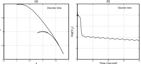
Figure 1. Response of the car model controlled using our proposed controller (69).
−1.5 −1 −0.5 0 0.5 1 −1
−0.5 0 0.5 1
x y
(a)
Homogeneous
0 10 20 30 40
−4 −2 0 2 4 6
Time (second)
log(V)
(b)
[image:10.595.374.476.367.426.2]Homogeneous
Figure 2. Response of the car model controlled using the sampled homogeneous controller (68).
Figure 1 shows the simulation results when the controller (69) is applied to control the plant in power form, and Figure 2 shows the response when the sample and hold version of controller (68), withk= 25/6, is applied. In
4
For consistency with Theorem 4.1, we have replaced the term sintwith costinu1 of [23].
the simulations we have usedx◦ = (0,0,0,1)0,T = 0.2 and= 0.35. We display the (x, y) position of the car and the log(VT) respectively. The (x, y) position of the car is given by the equationsx=x1andy=x4−x1x3+12x21x2.
Moreover, for comparison to the graph of log(VT) of Fig-ure 1(b), we have plotted log(V), where V = VT with
= 0, in Figure 2(b). It is shown that the proposed perturbed controller (69) performs very similarly to the homogeneous controller (68) in the absence of distur-bances. Note however that the controller (69) is in fact also a SP-ISS stabilizing controller for the same system with disturbance.
5.2 SP-ISS design for a unicycle mobile robot
Consider the model of a unicycle mobile robot moving on a plane, with two independent motorized wheels [22]:
˙
x=vcosθ+dsinθ; ˙y=vsinθ−dcosθ; ˙θ=ω, (70)
withv - the forward velocity,ω - the steering velocity, (x, y) - the Cartesian position of the center of mass of the robot,θ- the heading angle from the horizontal axis, and
d- a disturbance (exogenous force) perpendicular to the forward direction. Using the coordinate transformation
x1=x; x2= tanθ; x3 =−y+xtanθ ,we obtain the
model of system (70) in power form with disturbance:
˙
x1=u1+
d p
1 +x2 2
˙
x2=u2
˙
x3=x1u2+d
q 1 +x2
2,
(71)
where u1 := vcosθ, and u2 := ωsec2θ. Note that for
system (71), the exact discrete-time model is not com-putable explicitly. Choosing
W = 0.5x4
2+ 104x23andρ(W) = 0.1 4
p |W|,
it can be shown that the controller
u1T =−2x1+ρ(W)(cos((k+ 1)T)−
2sin((k+ 1)T))
u2T =−0.05 sign(Lf2W)|Lf2W|
α
2ρ(W) (72) + 2(2x1+ρ(W) cos((k+ 1)T)) cos((k+ 1)T)
−2x1sin((k+ 1)T)
,
and the Lyapunov function
VT = (2x1+ρ(W) cos((k+ 1)T)2+ρ(W)2
−2x1ρ(W) sin((k+ 1)T)
(73)
is a SP-ISS pair for the closed-loop system which consist of the Euler model of (71) with the controller (72).
[image:10.595.45.282.488.594.2]the (x, y) position5, which is given by the equations
x=x1andy=x1x2−x3. In the simulation, we use the
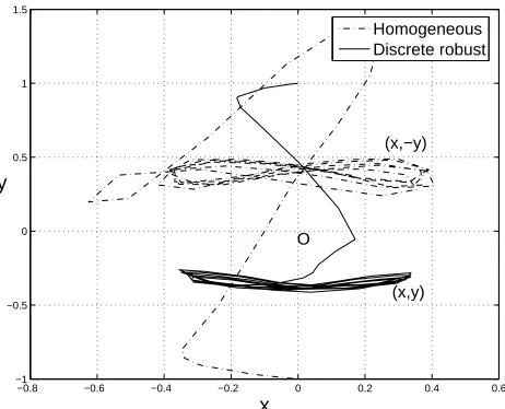
initial conditionx0= (0, 0, −1)T,T = 0.5 and= 13..
The simulation shows that, for the chosen parameters, the position of the vehicle is closer to the origin when ap-plying the proposed controller (72). This indicates that compared to the homogeneous controller, our proposed controller performs somewhat better in the presence of a disturbance. This behaviour is consistent for other sim-ulation settings with a careful choice of parameters of the controller.
−0.8 −0.6 −0.4 −0.2 0 0.2 0.4 0.6 −1
−0.5 0 0.5 1 1.5
x y
Homogeneous Discrete robust
O
(x,−y)
[image:11.595.48.279.204.391.2](x,y)
Figure 3. Position (x, y) with robust controller (72) vs posi-tion (x,−y) with homogeneous controller (upside down), for
d= 0.2.
6 Summary
We have presented a converse Lyapunov theorem for SP-ISS for parameterized discrete-time time-varying sys-tems. We have also presented an application of our result to discrete-time time-varying periodic systems and have applied this result to solve a discrete-time robust sta-bilization problem for nonholonomic systems in power form. We have proposed a construction of a discrete-time SP-ISS control law and a strict Lyapunov function. Design examples show that robust stabilization using continuous control is possible, and this gives an alter-native to emulation design for sampled-data stabiliza-tion for systems in power form. Moreover, since the ex-act discrete-time model of the nominal systems in power form can be explicitly computed, designing a discrete-time asymptotically (and robustly) stabilizing controller for the systems based on the exact discrete-time model and comparing the performance of the controller with the result of this paper would be an interesting topic for further research. Finally, the applicability of our method
5
Note that in Figure 3, in order to give a clear comparison, we plot the (x, y) position of the mobile robot controlled by the robust controller, and plot the (x,−y) position of the mobile robot when applying the homogeneous controller.
to more general classes of nonholonomic systems would also be an interesting direction to investigate.
Acknowledgements
This research was supported by the EPSRC Portfolio Award, Grant No. GR/S61256/01. The work of A. As-tolfi is partly supported by the Leverhulme Trust. The authors are grateful to the reviewers for their construc-tive comments.
References
[1] R. W. Brockett. Asymptotic stability and feedback stabilization. In R. W. Brockett, R. S. Millman, and H. J. Sussmann, editors, Differential Geometric Control Theory, pages 181–191. Birkhauser, Boston, 1983.
[2] J. M. Coron. Global asymptotic stabilization for controllable systems without drift.Math. of Control Signals and Systems, 5:295–312, 1992.
[3] H. A. Edwards, Y. Lin, and Y. Wang. On input to state stability for time varying nonlinear systems. InProc. IEEE Conf. Decis. Contr., volume 4, pages 3501–3506, Sydney, Australia, 2000.
[4] J. M. Godhavn and O. Egeland. A Lyapunov approach to exponential stabilization of nonholonomic systems in power form. IEEE Trans. Auto. Contr., 42:1028–1032, 1997. [5] Z. P. Jiang and Y. Wang. Input-to-state stability for
discrete-time nonlinear systems. Automatica, 37:857–869, 2001. [6] Z. P. Jiang and Y. Wang. A converse Lyapunov theorem
for discrete-time systems with disturbances. Systems and Control Letters, 45:49–58, 2002.
[7] D. S. Laila, D. Neˇsi´c, and A. R. Teel. Open and closed loop dissipation inequalities under sampling and controller emulation. European Journal of Control, 8:109–125, 2002. [8] Y. Lin. Input to state stability with respect to noncompact
sets. In 13th IFAC World Congress, pages 73–78, San Francisco, 1996.
[9] Y. Lin, E. D. Sontag, and Y. Wang. A smooth converse Lyapunov theorem for robust stability.SIAM J. Contr. Opt., 34:124–160, 1996.
[10] D. A. Lizarraga, P. Morin, and C. Samson. Non-robustness of continuous homogeneous stabilizers for affine control systems. In Proc. 38th IEEE Conf. Decis. Contr., pages 855–860, Arizona, 1999.
[11] P. Lucibello and G. Oriolo. Robust stabilization via iterative state steering with an application to chained form systems. Automatica, 37:71–79, 2001.
[12] R. T. M’Closkey and R. M. Murray. Exponential stabilization of driftless nonlinear control systems using homogeneous feedback. IEEE Trans. Automat. Control, 42:614–628, 1997. [13] S. Monaco and D. Normand-Cyrot. An introduction to motion planning under multirate digital control. In Proc. 31st IEEE Conf. Decis. Contr., pages 1780–1785, Tucson, Arizona, 1992.
[14] P. Morin and C. Samson. Exponential stabilization of nonlinear driftless systems with robustness to unmodelled dynamics. Control, Optim. and Calc. Variations, 4:1–35, 1999.
[16] D. Neˇsi´c and D. S. Laila. A note on input-to-state stabilization for nonlinear sampled-data systems. IEEE Trans. Auto. Contr., 47:1153–1158, 2002.
[17] D. Neˇsi´c and A. Loria. On uniform asymptotic stability of time-varying parameterized discrete-time cascades. IEEE Trans. Automat. Contr, 49:June, 2004.
[18] D. Neˇsi´c and A. R. Teel. Input-to-state stability for nonlinear time-varying systems via averaging. Math. Control, Signals and Systems, 14:257–280, 2001.
[19] D. Neˇsi´c and A. R. Teel. A framework for stabilization of nonlinear sampled-data systems based on their approximate discrete-time models.IEEE Trans. Auto. Contr., June, 2004. [20] D. Neˇsi´c, A. R. Teel, and P. Kokotovi´c. Sufficient conditions for stabilization of sampled-data nonlinear systems via discrete-time approximations.Syst. Contr. Lett., 38:259–270, 1999.
[21] D. Neˇsi´c, A. R. Teel, and E. Sontag. Formulas relating
KL stability estimates of discrete-time and sampled-data nonlinear systems.Syst. Contr. Lett., 38:49–60, 1999. [22] J. B. Pomet. Explicit design of time-varying stabilizing
control laws for a class of controllable systems without drift. Systems and Control Letters, 18:147–158, 1992.
[23] J. B. Pomet and C. Samson. Time-varying exponential stabilization of nonholonomic systems in power form. In Proc. of IFAC Symp. Robust Control Design, pages 447–452, Rio de Janeiro, 1994.
[24] C. Prieur and A. Astolfi. Robust stabilization of chained systems via hybrid control. IEEE Trans. Auto. Contr., 48:1768–1772, 2003.
[25] E. D. Sontag. Smooth stabilization implies coprime factorization. IEEE Trans. Auto. Contr., 34:435–443, 1989. [26] E. D. Sontag. Feedback stabilization of nonlinear systems.
In M. A. Kaashoek et al., editor,Robust Control of Linear Systems and Nonlinear Control, Proceedings of the Internat. Symp. MTNS-89, pages 61–81. Birkhauser, 1990.
[27] E. D. Sontag. The ISS philosophy as a unifying framework for stability-like behaviour. In A. Isidori, F. Lamnabhi-Lagarrigue, and W. Respondek, editors,Nonlinear Control in the Year 2000, Lecture Notes in Control and Information Sciences, volume 2, pages 443–468. Springer, Berlin, 2000.
[28] O. J. Sordalen. Conversion of the kinematics of a car withn
trailers into a chained form. InProc. of Internat. Conf. on Robotics and Automat., pages 382–386, Atlanta, 1993.
[29] O. J. Sordalen and O. Egeland. Exponential stabilization of nonholonomic chained systems. IEEE Trans. Auto. Contr., 40:35–49, 1995.
[30] A. M. Stuart and A. R. Humphries.Dynamical Systems and Numerical Analysis. Cambridge Univ. Press, 1996.
[31] A. R. Teel, R. M. Murray, and G. Walsh. Nonholonomic control systems: from steering to stabilization with sinusoids. InProc. IEEE Conf. Decis. Contr, pages 1603–1609, Tucson, AZ, 1992.