Algorithm based comparison between the integral method and
harmonic analysis of the timing jitter of diode-based and solid-state
pulsed laser sources
N.K. Metzger
a,n, C.-R. Su
b, T.J. Edwards
b, C.T.A. Brown
baSUPA School of Engineering and Physical Sciences, Photonics & Quantum Sciences, Heriot Watt University, Edinburgh EH14 4AS, UK bSUPA School of Physics and Astronomy, University of St Andrews, North Haugh, St Andrews, Fife KY16 9SS, UK
a r t i c l e i n f o
Article history: Received 21 August 2014 Received in revised form 25 November 2014 Accepted 27 November 2014 Available online 3 December 2014
Keywords: Phase noise Timing jitter Semiconductor lasers Mode-locked lasers Pulsed laser noise Pulse train Laser stabilization
a b s t r a c t
A comparison between two methods of timing jitter calculation is presented. The integral method uti-lizes spectral area of the single side-band (SSB) phase noise spectrum to calculate root mean square (rms) timing jitter. In contrast the harmonic analysis exploits the uppermost noise power in high harmonics to retrieve timingfluctuation. The results obtained show that a consistent timing jitter of 1.2 ps is found by the integral method and harmonic analysis in gain-switched laser diodes with an external cavity scheme. A comparison of the two approaches in noise measurement of a diode-pumped Yb:KY(WO4)2passively mode-locked laser is also shown in which both techniques give 2 ps rms timing jitter.
&2014 The Authors. Published by Elsevier B.V. This is an open access article under the CC BY license (http://creativecommons.org/licenses/by/3.0/).
1. Introduction
Actively and passively mode-locked lasers are ideal candidates for the generation of coherent, stable and highly periodical pulse trains. They have been the subject of intense investigation as they can be used in many applications, including high-speed optical communications, all-optical signal-processing, optical sampling and clock distribution[1]. Among these applications, some require not only high peak power and short pulse operation, but also the smallest possible timing jitter, as thefluctuation of the time in-terval between pulses degrades the quality of the expected system performance.
A broad bandwidth oscillator can detect timingfluctuations by monitoring the beat frequency between a modulated signal and low-jitter electrical trigger signal [2]. This enables one to easily obtain the exact timingfluctuation of an unknown optical source. Although this is an accurate method to calculate timing jitter, the equipment requirement of a broad bandwidth and a trigger-de-pendent source limits the practicality of such spectral measure-ments. These drawbacks can be overcome with the combination of a fast photodetector and an electronic spectrum analyzer. The
available bandwidth of the spectrum analyzer not only facilitates measurements, but also provides important insight into sources of both correlated and uncorrelated timing jitter[2,3].
By considering the noise sideband of the power spectrum, phase noise can be distinguished from amplitude fluctuation. Whilst phase noise rises quadratically with harmonic order, am-plitude fluctuation remains order independent across the full frequency spectrum[2]. Both of these effects contribute to ped-estals or broad noise sidebands that prevent a clean RF signal. The single side-band (SSB) phase noise, which is identified by the carrier per resolution bandwidth, reveals information about the timing jitter. Following von der Linde's work[2], the rms timing
fluctuation at a given carrier frequencyfRcan be obtained from a
spectral integration of noise if the rms amplitude noise remains small.
When using this method the integration boundaries need to be chosen carefully[4–12]to obtain high measurement accuracy. To solve this problem, an approach using a simplified theoretical model has been developed[2]. The harmonic approach adjusts the integration by utilizing the uppermost noise power to identify the timing jitter in higher harmonic orders. This has been verified as a valid solution[9,10], yet it remains relatively little used compared to the integration method discussed above. This is because the accuracy of harmonic analysis is greatly restricted by the highest Contents lists available atScienceDirect
journal homepage:www.elsevier.com/locate/optcom
Optics Communications
http://dx.doi.org/10.1016/j.optcom.2014.11.088
0030-4018/&2014 The Authors. Published by Elsevier B.V. This is an open access article under the CC BY license (http://creativecommons.org/licenses/by/3.0/).
nCorresponding author. Fax:þ44 131 451 3473.
harmonic order obtained; the higher the harmonic order, the more precise the timing jitter.
To date, a thorough comparison of both methods has yet to be conducted, despite Ng et al.[11]and Yoshida[12]confirming the consistent outcome of these two approaches in their own system. This publication presents two studies of the rms timing jitter calculated by the integral method as well as the harmonic analysis approach in gain-switched semiconductor laser diodes. The cal-culated timing jitter of 1.1 ps and 1.25 ps obtained by harmonic analysis and integral method respectively in this work, proved comparable to the 1.5 ps jitter in a Fabry–Perot gain-switched semiconductor laser diode with optical feedback [13,14]. These two algorithms were then applied to an Yb:KYW passive mode-locked lasers and yielded a free-running jitter time of 2.05 ps and 1.95 ps respectively. A similar agreement of results was obtained with an Yb:Eb:glass ultrafast laser[15].
The outcomes of this study validates the consistent measure-ment of timing jitter by both the harmonic analysis and integral method when tested theoretically and experimentally in mode-locked and gain-switched lasers.
2. Background to jitter measurements and algorithm development
The well-developed theory by von der Linde has been used to calculate rms timing jitter in spectral measurements[2]. This work analyzed the noise behavior in the power spectrum and found that noise varies with increasing harmonic orders. While amplitude noise remains a frequency-independent trend, phase noise in-creases quadratically and further becomes the main source of noise for high harmonics in RFSA. Phase noise is thus observed to have the largest contribution with respect to rms timing jitter. To compute timing jitter, there are two approaches advocated.
Thefirst approach, the integral method, uses the integration of the entire SSB phase noise to calculate the rms timing jitter. This approach assumes that the amplitudefluctuation is negligible in affecting the power spectrum. The second, harmonic analysis, is a simplified version of the integral method. This utilizes the whole power spectrum and then retrieves the uppermost noise power and full width at half maximum (FWHM) noise bandwidths in high harmonic orders for the calculation of rms timing jitter. Both methods have been validated to be correct theoretically and ex-perimentally[3,9,11,12,16,17].
In order to compare rms timing jitter efficiently, these two methods were implemented in Matlab. The content of these pro-grams for harmonic analysis and the integral method will be dis-cussed in the following sections.
2.1. Algorithm for harmonic analysis
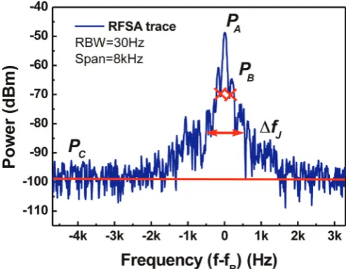
Before calculating rms timing jitter, harmonic analysis requires information from the RFSA trace. Afluctuation-free pulse train is seen to have a delta RF linewidth. However, once the pulse en-counters phase noise, an undefined phase relation between each pulse will result in the broadened linewidth RFSA trace shown in Fig. 1. After the red crosses (PB), the power spectrum encounters
noise interruption.
InFig. 1,PAdenotes the peak of the RFSA trace.PB andPC
re-present the power of the maximum noise level and the averaged noisefloor respectively.
The rms timing jitter can be estimated[2]with Eq.(1), given prior knowledge of parametersPA, PB,PC,
Δ
fresresolutionband-width (RBW),
Δ
fJ(the FWHM of noise bands), round trip timeT,and the harmonic ordernof the measured RFSA data in Eq.(1).
⎡ ⎣ ⎢ ⎢ ⎛ ⎝ ⎜ ⎞ ⎠ ⎟ ⎤ ⎦ ⎥ ⎥ t T n P
P f f (2 ) (1) B A n J res 1/2 π Δ = Δ Δ
where
Δ
tsymbolizes the rms timing jitter.PBthe uppermost noiselevel (red crosses in Fig. 1) is determined automatically as illustrated inFig. 2.
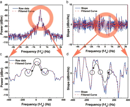
Initially, the unprocessed RFSA data is convoluted with a moving average filter generated by the analysis program to re-move spurious aliasing ripples. From thisfiltered curveFig. 2(a), the algorithm is able to extract its slope. The slope of the raw RFSA data and itsfiltered curve slope are both depicted inFig. 2(b) by the blue curve and red dotted curve, respectively. Looking back at the original data inFig. 2(a), it can be seen that the uppermost phase noise has a local minima, shown in the expanded (c). Fur-thermore, the local maximum or minimum points inFig. 2(c) will have a value of approximately zero at the same frequencies in (d). It is not surprising that the extreme values usually result from the transition in slope. Therefore, to find the uppermost noise, the program can rely on the transition point of the slope. In other words, values where there are zero crossingsFig. 2(d) correspond to the extreme values of (c).
Similarly PA and PC can both be obtained from a standard
maximum and minimum search function wherePCwas taken as
the average noisefloor. The points (fJ1andfJ2) both have powers of (PBþPC)/2 in the power spectrum, where the corresponding
fre-quency distance between the two points determines the FWHM of the noise bandwidths
Δ
fJ¼fJ1–fJ2. Roundtrip timeT, harmonic or-dern, and RBW can be retrieved from the RFSA trace. This method assumes no correlations between the intensity and phase noise of the pulses[2]. When timing-jitterfluctuations between pulses are uncorrelated in time a Lorentzian shaped RFSA trace is obtained. Correlations between timingfluctuations tend to produce traces that are Gaussian in shape[6]. In thefirst case the accuracy of the prediction of the jitter will suffer however the algorithm will still give a fast qualitative prediction as shown in experimental section.2.2. Amplitudefluctuations
[image:2.595.303.550.58.250.2]Although amplitude noise remains a small value for most fre-quencies, it nevertheless influences the power spectrum regarding
Fig. 1.The RFSA trace obtained with Matlab (RBW¼30 Hz). The RFSA trace shows
lower harmonic orders[2]. Zero-order noise has especially been found to be influenced most by energy instability. This behavior is described below in Eq.(2)
⎡⎣ ⎤⎦
E E/ ( / )P PB A0 fA/ fres (2)
1/2
Δ = Δ Δ
where
Δ
E/Eis the amplitudefluctuation,PB is the maximum ofnoise level,PAis the peak power,
Δ
fAis the FWHM of the zeroorder noise bands and
Δ
fresis the resolution bandwidth. It can beseen that the equation is very similar to Eq.(1), except that the harmonic order is zero. Therefore the Matlab based harmonic analysis algorithm can be applied to evaluate energyfluctuation when the carrier frequency is set at DC.
2.3. Integral method
In a second approach the integral method was used to auto-matically determine the noise level. When using the integral method to calculate the timing jitter, it is necessary to obtain the SSB phase noise spectrum. The SSB phase noise spectrum,L(f), is defined as the ratio of noise in a 1 Hz resolution bandwidth at a specified frequency offset fto the oscillator signal amplitude at carrier frequencyfn. Eq.(3)illustrates this concept[16]
⎡ ⎣ ⎢ ⎢
⎤ ⎦ ⎥ ⎥ L f P f
P f ( ) log ( )
(3)
F
A res
10
=
Δ
where PF(f) is the SSB noise spectral density, PA is the carrier
power, and
Δ
fresresolution bandwidth (RBW). For higherharmo-nic orders,PF(f) will be dominated by the SSB phase noise spectral
densityPJ(f)[16]. WhereL(f) is obtained from the RFSA trace in
units of dBc/Hz. The spectral area of the power spectrum can be directly related to the timingfluctuation by Eq.(4)
t
f L f df L f df 1
2 ( ) ( ) (4)
j
n f f
f f
f f f f
n min
n max
n max
n min
∫
∫
π
= +
+ +
− −
wherefnis the carrier frequency at harmonic ordern,L(f) is the
SSB phase noise spectrum, andtjis the rms timing jitter. In the
equation, fmax and fminare the upper and lower boundaries for
integration.
Because of its simple numerical formula, the integral method is most commonly used for calculating timing jitter. An algorithm for the integration method can be implemented by simply performing integration via the trapezoidal method.
Despite being a convenient way to determine timing jitter, care has to be taken when defining the integration boundaries fmax
(upper boundary) andfmin(lower boundary)[2].
In this work the lower integration boundary (fmin) was
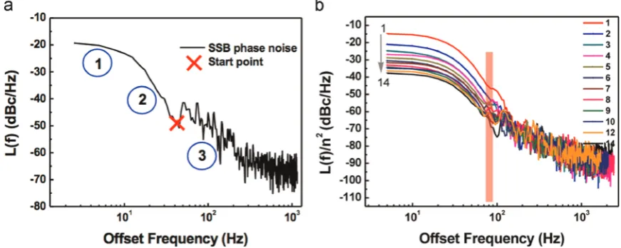
de-termined through the aid of the harmonic algorithm. Fig. 3 (a) shows the 14th order SSB phase noiseL(f) in the RF spectrum. The red cross representsPBthe power of the maximum noise level
[image:3.595.86.519.57.414.2]as used for the harmonic analysis. InFig. 3(b) the normalizedL(f) from harmonic orders 1–14 is shown.
Fig. 2.The illustration of harmonic analysis (a) the raw RFSA trace (blue curve) and thefiltered curve (red dashed line) with a RBW of 30 Hz. (b) The slope of the RFSA data
The curve inFig. 3(a) can be divided into three regions. Thefirst section from 5 Hz to 20 Hz displays a white plateau as marked 1. The second section ranging from 20 Hz to 40 Hz shows accelerated degradation. Beyond 40 Hz, the third section shows a decaying trend of 20 dBc/Hz per decade due to phase noise marked as 3. Fig. 3(b) demonstrates the respective normalized SSB phase noise with varying ordern. The lower integration boundary (fmin) are
within offset frequencies 80–90 Hz as highlighted in Fig. 3(b). After this the normalized SSB phase noise scales and aligns each other accordingly to their respective order numbernfrom 1 to 14. These lower boundaries were determined by the harmonic analysis algorithm as indicated by the red cross in Fig. 3(a). Ac-cording to the algorithm's search result, the pure signal and phase noise can be separated, thus demonstrating the viability of the Matlab algorithm to identify phase noise.
The upper integration boundaryfmaxhas an approximate limit.
Typicallyfmax is half the span[11,18] or the point where phase
noise hits the thermal noisefloor[4,19]. In the analysis presented here the upper integration boundary was selected to be at the intercept where the noise floor meets the phase noise, to be analogous with the harmonic analysis and the slope is not at 20 dBc/Hz per decade. In the following example this is illustrated:
the integral algorithm employedfmin¼0.5 kHz, found by the
har-monic algorithm as a lower integration boundary and the upper integration boundary wasfmax¼10 kHz as the intercept with the
noise floor. The noise floor therefore determines the upper boundary and hence thesefluctuations are not accounted for in the integral. This aids to reduce the contribution of amplitude
fluctuations to the analysis under the assumption that the timing jitter within the integral boarders is correlated and amplitude
fluctuations are small and do not affect the phase[2].Fig. 4 de-monstrates the resulting integration boundaries.
In the analysis shown inFig. 4, a jitter of 2.85 ps was obtained compared to a jitter value of 2.59 ps obtained for the same dataset using the Harmonic analysis. To check the robustness of our ap-proach several measurements were conducted from which a pre-cision of76% was estimated.
Integration of the entire area from fmin to half of the
mea-surement span as used in Refs.[18,20]results in an increase of the calculated jitter by about 15%, which is similar to[21]. Thus it can be seen that the spectral area related to phase noise is affected by the correct choice of fmax outside the thermal noise floor. The
[image:4.595.74.510.60.234.2]average noise floor (red line in Fig. 4(a)) was found to be 96.42 dBm whereasfmax(red circle inFig. 4(a)) was determined
Fig. 3.(a) The SSB phase noise spectrum (acquired with a RBW of 80 Hz) of harmonic ordern¼14 with three different slopes; (b) the normalized SSB phase noise depicted
[image:4.595.76.512.527.704.2]with varied harmonic orders fromn¼1 to 14. Withfminbeing within offset frequencies 80–90 Hz as highlighted in red. (For interpretation of the references to color in this figure legend, the reader is referred to the web version of this article.)
Fig. 4.(a) Harmonic analysis: The RFSA trace (with a RBW of 100 Hz) showsPB(red crosses) andPCthe average noisefloor as a red line as determined by the harmonic
to93.45 dBm by the integral analysis. Both values are reasonably close to each other and give confidence in the presented approach to determine the integration boundary. In the following work,fmin
was set to be equal to that used in the harmonic analysis to enable the comparison between the two approaches.
With these algorithms, we are now well placed to analyze different laser systems and compare their jitter values.
3. Application to picosecond pulses from a gain-switched ex-ternal cavity diode laser
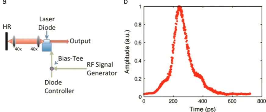
With the developed algorithm, we assessed the performance of a commercial GaAs tapered diode lasers from m2k-laser (TAL-1060-2000). The laser has a reflectivity 1% at the output facet and anti-reflection coating of 0.01% at the rear facet and was arranged in an external cavity geometry[22,23]as depicted inFig. 5(a). The laser was operated with a DC offset bias and a supplementary RF-modulated injection current from a signal generator. An electronic amplifier was incorporated to provide an RF power of 35 dBm. The output optical pulses centered at 1060 nm were detected using a fast InGaAs photodiode, which had a time response full-width at half-maximum (FWHM) of 12.5 ps. Care has to be taken not to oversaturate the sensitive detector as permanent damage might occur. For the experiments conducted here an average power of 0.5–0.6 mW was incident on the detector element. This was below the maximum value of 1 mW quoted by the manufacturer for save operation. By blocking the beam into the detector input it was ensured that the acquired RFSA trace was above the detector and RF analyzer noisefloor before each measurement. The pulse train was captured using a 22 GHz Radio Frequency Signal Analyzer that was computer interfaced.
The maximum output power is found to be 115 mW when operated at an injection current of 200 mA. The cavity length is chosen to be 23.2 cm give a pulse repetition frequency of 651.1 MHz. The best pulse quality requires a stable signal without any noise induced by self-pulsation. The RFSA trace is found to be Lorentzian shape when the DC current is maintained at 42 mA, and the RF frequency is set at 640.67 MHz. These results corre-spond to those obtained in similar gain-switched schemes[13]. With the parameters chosen above, the RFSA trace can be seen up to the 7th harmonic order in the system.
The jitter algorithm was applied to all seven harmonic orders.
The harmonic approach and integral method in the RF spectrum are depicted inFig. 6(a) and (b), respectively.
InFig. 6(a), the harmonic approach establishes the red starred points as the uppermost powers used to calculate timing jitter. FromFig. 6(b), the spectral area is calculated via integration from fmin¼0.9 kHz to fmax¼10 kHz and is further converted to timing
jitter by the integral method. Increasing of the integration border to the full acquisition spanfmax¼40 kHz results in an increase of
the timing jitter by 13% approximately 3% relative to the increased integration bandwidth indicating that the major contribution to the jitter is in the lower frequency components. Relaxation oscil-lations for modulated lasers can contribute to the timing jitter but are estimated to be higher than the jitter frequency range of ap-proximately 1–10 kHz considered here. Fig. 7(a) shows that the total phase noise determined by the harmonic and integral method is consistent. The two results both follow the linear ten-dency of
ϕ
(n)/ϕ
(1)¼n from orders 1 to 7. Consequently, a fre-quency-independent jitter is obtained from the two algorithms in Fig. 7(b).From Fig. 7(b), the average jitter [5] is determined to 1.270.2 ps and 1.270.2 ps for the harmonic and integral method respectively. This corresponds well to the value (1.5 ps) obtained in [13] where the single contact Fabry–Perot gain-switched semi-conductor laser diode is operated at twice the DC threshold cur-rent with an external cavity scheme. The reduced jitter, which differs from the typical value of the gain-switched edge emitting laser diode (41.5 ps experimentally and 43.5 ps theoretically [24]), is due to optical feedback, which has been verified to reduce timing jitter greatly[25]. This is because the high coherence of reflected photons suppresses the spontaneous emission of laser diodes [24]. In summary, both the harmonic approach and the integral method give consistent and accurate calculations of tim-ing jitter for this laser system.
4. Application to femtosecond pulses from an mode-locked Yb:KYW laser
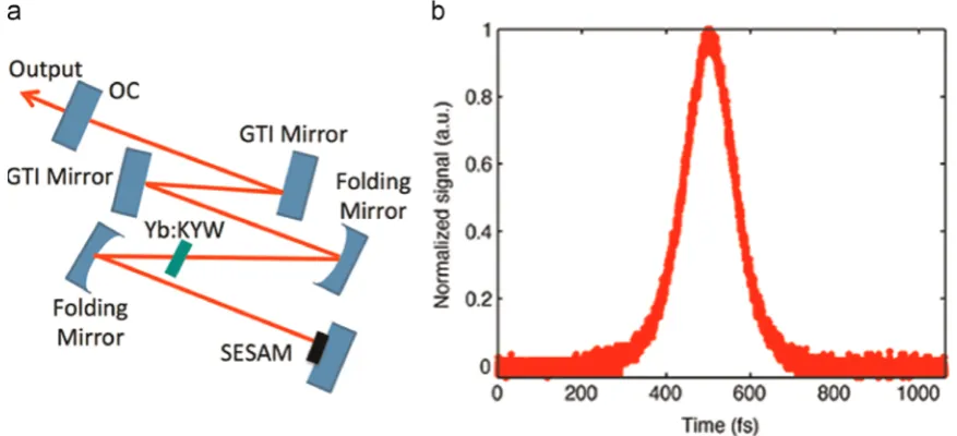
[image:5.595.82.519.530.714.2]We next applied the algorithm to passively mode-locked pulses from a solid state laser. The pulse source used was a diode-pumped Yb:KYW laser similar to the systems developed in[26,27]. The laser was passively mode-locked using a semiconductor sa-turable absorber mirror and produced of 138 fs duration in the
Fig. 5.(a) Layout of the gain-switched laser diode. The external cavity is formed between a HR high reflected mirror and the diode facet. Two 40microscope objectives are
Fig. 6.(a) The RFSA trace of the 7th order in gain-switched laser diode with a RBW of 100 Hz and span of 80 kHz (b) the SSB phase noise spectrum of 7th order with the lower integrationfmax¼10 kHz (circle) and the upper boundaryfmin¼900 Hz (cross). (For interpretation of the references to color in thisfigure, the reader is referred to the web version of this article.)
Fig. 7.(a) The rms phasefluctuation determined by the harmonic and integral method and plotted with the theoretical prediction line. (b) The measurement of timing jitter
by the two algorithms.
Fig. 8.(a) A schematic of the asymmetricz-fold Yb:KYW cavity. The folding mirrors are spherically curved with radii of curvature of 75 mm. SESAM is a semiconductor
saturable absorber mirror (A¼2% andΔR¼1.2%), while OC is a 3.2% output coupler. Both GTI mirrors provide a single pass dispersion of910 fs2
[image:6.595.73.512.515.715.2]1035–1040 nm wavelength range with a pulse repetition fre-quency of 161 MHz at an average output power of 80 mW. The corresponding spectral width for the pulses was 8.5 nm, which implied a time-bandwidth product of 0.33.
The schematic and a measured intensity autocorrelation trace of the mode-locked Yb:KYW laser are shown inFig. 8.
The output beam is coupled into the same measurement setup as in the previous section via an optical isolator to prevent feed-back. The highest harmonic order is found to be 22. In harmonic orders higher than 22, the phase noise interferes with the RFSA trace so strongly that the timing jitter cannot be distinguished.
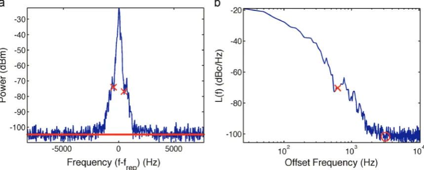
[image:7.595.88.518.61.233.2]A high RBW of 80 Hz and span of 20 kHz is chosen to prevent amplitudefluctuation from entering low harmonics. InFig. 9the RFSA trace and the resulting SSB trace for the 7th order are shown. InFig. 9(b), the noise band has a gradually descending slope in the SSB phase noise spectrum and is found that the noise skirt hits the noise floor at an offset frequency of approximately 3 kHz. Hence,fmax¼3.1 kHz is selected as a suitable upper boundary and fmin¼625 Hz is selected as the lower boundary.
Fig. 10(a) shows the evaluation of timing jitter when the am-plitude noise is taken to be negligible.Fig. 10(b) illustrates the total rms phase noise with varied harmonic orders.
InFig. 10(a), the linear trend also obeys the predicted theore-tical model detailed previously. In Fig. 10(b), the consistency of harmonic approach and integral method is demonstrated up to the
12th harmonic order. In higher harmonic orders, the phase noise interferes with the RFSA trace more strongly so that the timing jitter cannot be distinguished accurately and the results start to
fluctuate. The algorithms determine an average timing jitter[5]of 2.070.6 ps and 1.970.3 ps for the harmonic and integral method respectively for the different orders. This is a comparable value to the 2.5 ps obtained in a similar soliton mode-locked system[15]. Timing phase noise scales inversely with the intracavity pulse energy and linearly with the square of pulse duration [28]. The discrepancy of 0.5 ps can be explained from the interaction be-tween the lower pulse energy (0.5 nJ) and shorter pulse duration (138 fs) compared to the pulse energy (1.03 nJ) and pulse duration (255 fs) obtained in [15]. In conclusion, harmonic and integral method found an average timing jitter of approximately 2 ps, a value that is much larger than that obtained in active mode-locked systems[14]. To diminish the free-running timing jitter to a fem-tosecond jitter regime, feedback timing stabilization such as a phase-locked loop (PLL) system can be employed in the same mode-locked system scheme[29].
5. Conclusion
This publication presented thefirst direct comparison between the harmonic analysis and the integral method of characterizing
Fig. 9.(a) The RFSA trace for the 7th order with a RBW of 80 Hz, and (b) its SSB phase noise with the lower integrationfmax¼3.2 kHz (circle) and the upper boundaryfmin
[image:7.595.87.519.281.451.2]¼625 Hz (cross).
Fig. 10.The timing jitter measurements of a Yb:KYW mode-locked laser (a) the total phase noisefluctuation and (b) the timing jitter of different harmonic orders calculated
timing jitter. The study of both approaches used the theoretical framework developed by von der Linde[2]that has been widely used in RF measurement, and investigated using an automated Matlab program[30]. The algorithm results show that both the harmonic approach and the integral method correspond to the theory appropriately and are reliable in characterizing rms timing jitter. Noise estimation in gain-switched laser diode and Yb:KYW passive mode-locked solid state laser are used to thoroughly compare the two methods.
The applied method relies on direct detection of the pulse train and therefore the dynamic range of the detector limits phase noise measurement of the RF harmonic. These limitations are overcome by employing the optical cross-correlation method [31]. In con-trast to the approach applied in this publication it is an all-optical timing jitter characterization method that enables extremely high timing resolution. The optical cross-correlation method has re-cently been employed for ultralow timing jitter measurement[32] in solid state lasers and also shows good agreement with the in-tegral method when applied to mode-locked laser diodes[33].
Nevertheless the outcomes not only demonstrate a consistent relationship between the two methods but also prove their accu-racy in evaluating rms timing jitter, as the values have been
con-firmed experimentally and theoretically in the same system setup.
Acknowledgments
This work was supported by the European Metrological Re-search Programme EMRP under IND 14. The EMRP is jointly fun-ded by the EMRP participating countries within EURAMET and the European Union. N.K. Metzger acknowledges support from the EPSRC Centre for Innovative Manufacturing in Laser-based Pro-duction Processes, funded through EPSRC grant EP/K030884/1.
References
[1]E.A. Avrutin, J.H. Marsh, E.L. Portnoi, Monolithic and multi-GigaHertz mode-locked semiconductor lasers: constructions, experiments, models and appli-cations, IEEE Proc.—Optoelectron. 147 (2000) 251–278.
[2]D. von der Linde, Characterization of the noise in continuously operating mode-locked lasers, Appl. Phys. B 39 (1986) 201–217.
[3]D.A. Leep, D.A. Holm, Spectral measurement of timing jitter in gain-switched semiconductor lasers, Appl. Phys. Lett. 60 (1992) 2451–2453.
[4]J.P. Tourrenc, A. Akrout, K. Merghem, A. Martinez, F. Lelarge, A. Shen, G. H. Duan, A. Ramdane, Experimental investigation of the timing jitter in self-pulsating quantum-dash lasers operating at 1.55mm, Opt. Exp. 16 (2008) 17706–17713.
[5]C.Y. Lin, F. Grillot, Y. Li, R. Raghunathan, L.F. Lester, Microwave characterization and stabilization of timing jitter in a quantum-dot passively mode-locked laser via external optical feedback, IEEE J. Sel. Top. Quantum Electron. 17 (2011) 1311–1317.
[6]D. Eliyahu, R.A. Salvatore, A. Yariv, Effect of noise on the power spectrum of passively mode-locked lasers, J. Opt. Soc. Am. B 14 (1997) 167–174. [7]B. Zhu, I.H. White, K.A. Williams, M.R.T. Tan, R.P. Schneider Jr, S.W. Corzine, S.
Y. Wang, Ultralow timing jitter picosecond pulse generation from electrically gain-switched oxidized vertical-cavity surface-emitting lasers, IEEE Photonics Technol. Lett. 9 (1997) 1307–1309.
[8]M. Schell, W. Utz, D. Huhse, J. Kässner, D. Bimberg, Low jitter single-mode pulse generation by a self-seeded, gain-switched fabry-perot semiconductor-laser, Appl. Phys. Lett. 65 (1994) 3045–3047.
[9]M. Jinno, Correlated and uncorrelated timing jitter in gain-switched laser-diodes, IEEE Photonics Technol. Lett. 5 (1993) 1140–1143.
[10]A. Martinez, S. Yamashita, Multi-gigahertz repetition rate passively mod-elockedfiber lasers using carbon nanotubes, Opt. Exp. 19 (2011) 6155–6163. [11]W. Ng, Y.M. So, R. Stephens, D. Persechini, Characterization of the jitter in a
mode-locked Er-fiber laser and its application in photonic sampling for ana-log-to-digital conversion at 10 Gsample/s, J. Lightwave Technol. 22 (2004) 1953–1961.
[12]E. Yoshida, M. Nakazawa, Measurement of the timing jitter and pulse energy fluctuation of a PLL regeneratively mode-lockedfiber laser, IEEE Photonics Technol. Lett. 11 (1999) 548–550.
[13]K.A. Williams, I.H. White, D. Burns, W. Sibbett, Jitter reduction through feed-back for picosecond pulsed InGaAsP lasers, IEEE J. Quantum Electron. 32 (1996) 1988–1994.
[14]D.J. Derickson, P.A. Morton, J.E. Bowers, R.L. Thornton, Comparison of timing jitter in external and monolithic cavity mode-locked semiconductor-lasers, Appl. Phys. Lett. 59 (1991) 3372–3374.
[15]G.J. Spühler, L. Krainer, E. Innerhofer, R. Paschotta, K.J. Weingarten, U. Keller, Soliton mode-locked Er:Yb:glass laser, Opt. Lett. 30 (2005) 263–265. [16]K.K. Gupta, D. Novak, H.F. Liu, Noise characterization of a regeneratively
mode-lockedfiber ring laser, IEEE J. Quantum Electron. 36 (2000) 70–78. [17]M.J.W. Rodwell, D.M. Bloom, K.J. Weingarten, Subpicosecond laser timing
stabilization, IEEE J. Quantum Electron. 25 (1989) 817–827.
[18]U. Keller, K.D. Li, M.J.W. Rodwell, D.M. Bloom, Noise characterization of fem-tosecondfiber raman soliton lasers, IEEE J. Quantum Electron. 25 (1989) 280–288.
[19]G. Serafino, P. Ghelfi, P. Pérez-Millán, G.E. Villanueva, J. Palací, J.L. Cruz, A. Bogoni, Phase and amplitude stability of EHF-band radar carriers generated from an active mode-locked laser, J. Lightwave Technol. 29 (2011) 3551–3559. [20]A. Finch, X. Zhu, P.N. Kean, W. Sibbett, Noise characterization of mode-locked
color-center laser sources, IEEE J. Quantum Electron. 26 (1990) 1115–1123. [21]M.J.R. Heck, E.J. Salumbides, A. Renault, E.A.J.M. Bente, Y.-S. Oei, M.K. Smit, R. van Veldhoven, R. Nötzel, K.S.E. Eikema, W. Ubachs, Analysis of hybrid mode-locking of two-section quantum dot lasers operating at 1.5μm, Opt. Exp. 17 (2009) 18036.
[22]P.J. Delfyett, L.T. Florez, N. Stoffel, T. Gmitter, N.C. Andreadakis, Y. Silberberg, J. P. Heritage, G.A. Alphonse, High-power ultrafast laser-diodes, IEEE J. Quantum Electron. 28 (1992) 2203–2219.
[23]P.J. Delfyett, High-power ultrafast semiconductor-laser diodes, Ultrafast Pulse Gener. Spectrosc. 1861 (1993) 72–83.
[24]M.R.H. Daza, C.A. Saloma, Jitter dynamics of a gainswitched semiconductor laser under self-feedback and external optical injection, IEEE J. Quantum Electron. 3 (2001) 254–264.
[25]E.H. Bottcher, D. Bimberg, Detection of pulse to pulse timing jitter in peri-odically gain-switched semiconductor-lasers, Appl. Phys. Lett. 54 (1989) 1971–1973.
[26]N.K. Metzger, W. Lubeigt, D. Burns, M. Griffith, L. Laycock, A.A. Lagatsky, C.T. A. Brown, W. Sibbett, Ultrashort-pulse laser with an intracavity phase shaping element, Opt. Exp. 18 (2010) 8123–8134.
[27]A.A. Lagatsky, E.U. Rafailov, C.G. Leburn, C.T.A. Brown, N. Xiang, O. G. Okhotnikov, W. Sibbett, Highly efficient femtosecond Yb:KYW laser pumped by single narrow-stripe laser diode, IEEE Electron. Lett. 39 (2003) 1108–1110.
[28]R. Paschotta, Noise of mode-locked lasers (Part II): timing jitter and other fluctuations, Appl. Phys. B 79 (2004) 163–173.
[29]H. Tsuchida, Pulse timing stabilization of a mode-locked Cr:LiSAF laser, Opt. Lett. 24 (1999) 1641–1643.
[30] N.K. Metzger,〈http://home.eps.hw.ac.uk/km359/commercial.html〉(August 2014).
[31]L.A. Jiang, A. Leaf, M.E. Grein, H. Haus, E.P. Ippen, Noise of mode-locked semiconductor lasers, IEEE J. Sel. Top. Quantum Electron. 7 (2001) 159–167. [32]A.J. Benedick, J.G. Fujimoto, F.X. Kärtner, Opticalflywheels with attosecond
jitter, Nat. Photonics 6 (2012) 97–100.