Parallel processor implementation in computerized tomography using transputers : a thesis presented in partial fulfilment of the requirement for the degree of Master of Technology in Production Technology at Massey University

PARALLEL PROCESSOR IMPLElVIENTATION

IN COMPUTERIZED TOMOGRAPHY USING

TRANSPUTERS

A THESIS PRESENTED IN PARTIAL FUFILMENT OF THE

REQUIREMENT FOR THE DEGREE OF MASTER OF TECHNOLOGY IN PRODUCTION TECHNOLOGY AT MASSEY UNIVERSITY

WENJUWU

Abstract

Acknowledgements

I wish to express my sincere appreciation to my supervisor, Dr. Bob Chaplin, for his guidance throughout this project.

I would like to thank Prof Bob Hodgson and Dr Bob Chaplin for their help and care during the course ofmy study, Dr Roger Browne for his help throughout the project and Mr White Page for his help in image research.

My thanks also extend to Dr Paul Austin, Dr Huub Bakker, Mr Ralph Pugmire, Dr Clive Marsh, Mr Merv Foot and all staff in the Production Technology Department of Massey University for their help and friendship.

I wish to gratefully acknowledge Mr Phil Long for all his help during my research period.

Table of Contents

Abstract .. ... ... .. .. .. . . ... .. . . .. . .. . ... . ... . ... ... ... ... 11

Acknowledgements . ... . . . ... . .. .. ... ... ... ... 111

Table of Contents . . . .. . . .. . . . .. . . . .. . . . .. .. . .... .. . . . ... ... .... .... ... . .. ... 1v

List of Figures . . . .. . . .. . ... .. . . .. . . .. . . .. .. . . . .. ... . . .. . . . ... ... VIII Chapter 1 Introduction to X-Ray Computerized Tomography... 1

1.1 Digital Image Processing... 1

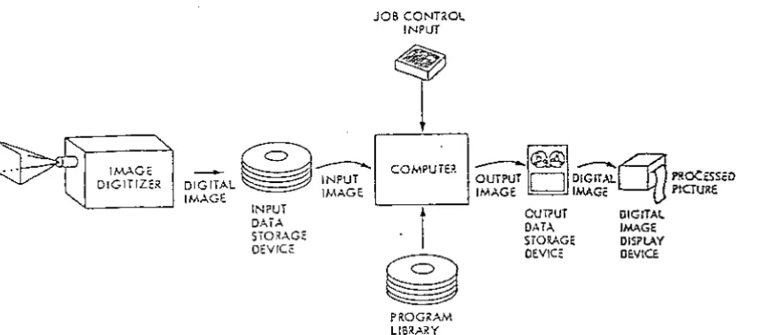
1.1.1 The elements of digital image processing ... 2

1.1.2 Basic classes of digital image processing ... .... ... 3

1.2 The Fundamentals of Computerized Tomography ... 7

1.2.1 Theoretical background for image reconstruction ... 9

1.2.1.1. The N-Dimensional Continuous Fourier Transform ( CFT) . ... .. . . .. .. . .. . . . .. .. . . .. .. . . ... . .. ... 9

1.2.1.2. The N-Dimensional Discrete Fourier Transform (DFT) ... 11

1.2.1.3. Projections... 14

1.2.1.4. The Projection-Slice Theorem ... 15

1.2.1.6. Reduction of the Dimensionality of the

Reconstruction Problem .. .. . ... .. .. .. .. .. .. .. .. .. .. . . ... ... .. 18

Chapter 2 Introduction to Parallel Processing and Transputers ... 19

2.1 The Principles of Parallel Processing Systems... 19

2.2 Description of Parallel Processes ... ... 22

2.2.1 Initiation and termination mechanisms... 23

2.2.2 Synchronization mechanism ... 23

2.2.3 Protection mechanism ... 24

2.2.4 Communication mechanism ... 24

2.3 The Transputers . . . .. . . .. .. .. .. .. . . .. .. . .. .. .. . .. ... .. .. ... . . .. . . ... ... 25

2.3.1 Overview ... .. ... 25

2.3.2 Occam ... ... 27

2.3.3 Communication channels... 30

Chapter 3 Reconstruction Algorithms for Parallel and Fan Beam Projections . . . . .. . . .. . . .. . . ... ... .. ... ... 32

3.1 Reconstruction Algorithm for Parallel Projections... 32

3.1.1 The idea ... 32

3.1.2 Theory ... ... ... ... ... ... 35

3.3 Modified Backprojection Algorithm... 44

Chapter 4 Parallel Processor Implementation in Computerized Tomography using Transputers . . . ... ... . . .. .. . . . ... . ... ... .. . .. .. 52

4.1 Analysis of the Reconstruction Algorithm... 52

4.2 IMS T414 Transputer... 57

4.2.1 Pin designations . . . .. . . .... ... .. . ... ... 59

4.2.2 Processor ... 60

4.2.3 Communications ... 62

4.2.4 Timers . . .. . . .. . .. . . ... . . ... ... .... ... 63

4.3 The Structure of the Transputer Network... 63

4.4 Connectivity of the Transputer System ... 65

4.4.1 Topology of transputer system ... 67

4.5 Algorithm Structure ... 69

4.5.1 Convolution ... .. ... 69

4.5.2 Backprojection ... 70

4.5.3 Interpolation .... ... 70

4.6 Implementation Details ... 71

4.6.2 Algorithm implementation in multiple transputer

network system .. ... ... ... ... 72

Chapter 5 Conclusion ... 78

References... 79

List of Figures

Fig. 1-1 A digital image processing system... 3

Fig. 1-2 Image representation and modelling... 4

Fig. 1-3 Image reconstruction using x-ray CT scanners... 7

Fig. 1-4 Typical chest x-ray radiograph ... 8

Fig. 1-5 The relationship between the projection of a two-dimensional function and slice of its Fourier transform ... 17

Fig. 2-1 Diagram to show that two summations can be performed in parallel ... 21

Fig. 2-2 Block diagram of the transputer ... 26

Fig. 2-3 Processes of a transputer ... .. .. .. .... ... .... ... ... 27

Fig. 3-1 Filter process ... 33

Fig. 3-2 Backprojection reconstruction... 36

Fig. 3-3 The ideal filter response for the filtered backprojection algorithm 38 Fig. 3-4 The impulse response of the filter shown in Fig. 3-3 ... .. 39

Fig. 3-5 Fan beam projections ... .. 41

Fig. 3-6 Fan and parallel beam projections ... .. 43

Fig. 3-8 Block diagram of the hardware for a single block of the systolic

array... 49

Fig. 3-9 The blocks in systolic arrays .. .. .. ... 50

Fig. 3-10 The new block diagram of the hardware for a single block of the systolic array... 51

Fig. 4-1 IMS T414 block diagram... 58

Fig. 4-2 Linked process list ... 61

Fig. 4-3 The arrangement of transputer network... 65

Fig. 4-4 Link names and addresses ... .. .... .. ... 66

Fig. 4-5 Block diagram of target system .. ... ... 68

Fig. 4-6 The communication structure of the transputer network ... 69

Fig. 4-7 Polar coodinate reconstruction geometry ... ... ... ... 7 4 Fig. 4-8 Cartesian reconstruction geometry... 75

CHAPTER 1. INTRODUCTION TO X-RAY COMPUTERIZED TOMOGRAPHY

Tomography refers to the cross-sectional imaging of an object from either transmission or reflection data collected by illuminating the object from many different directions. The impact of this technique in diagnostic medicine has been revolutionary, since it has enabled doctors to view internal organs with unprecedented precision and with safety for the patient. The first medical application utilized x-rays for forming images of tissues based on their x-ray attenuation coefficient. More recently, however, medical imaging has also been successfully accomplished with radioisotopes, ultrasound, and magnetic resonance; the image parameter being different in each case.

There are numerous nonmedical imaging applications which lend themselves to the methods of computerized tomography. Researchers have already applied this methodology to the mapping of underground resources via crossborehole imaging, some specialized cases of cross-sectional imaging for nondestructive testing, the determination of the brightness distribution over a celestial sphere, and three-dimensional imaging with electron microscopy.

Fundamentally, tomographic imaging deals with reconstructing an image from its projections. It is an important part of Digital Image Processing. In this chapter, we firstly introduce some basic idea about Digital Image Processing. Then the fundamentals of computerized tomography will be discussed.

1.1 Digital hnage Processing

speed and storage capabilities required for practical implementation of image processing algorithms. Since then, this area has experienced vigorous growth, having been a subject of interdisciplinary study and research in such fields as engineering, computer science, information science, statistics, physics, chemistry, biology, and medicine. The results of these efforts have established the value of image processing techniques in a variety of problems ranging from restoration and enhancement of space-probe pictures to processing of fingerprints for commercial transactions. Several new technological trends promise to further promote digital image processing. These include parallel processing made practical by low-cost microprocessors, and the use of charge-coupled devices (CCDs) for digitizing, Storage arrays. Another impetus for development in this field stems from some exciting new applications on the horizon. Certain types of medical diagnosis, including differential blood cell counts and chromosome analysis, are a state of practicality by digital techniques. The remote sensing programs are well suited for digital image processing techniques. Thus, with increasing availability of reasonably inexpensive hardware and some very important applications on the horizon, one can expect digital image processing to continue its phenomenal growth and to play an important role in the future.

1.1.1 The Elements of Digital hnage Processing

IMAGE DIGITIZER

JOB CONHOL

INPUT

1

___,... INPUT ourPur

D

DIGITAL no<:osco

DIGITAL IMAGE IMAGE IMAG- PICTURE

IMAGE c

~ [ COMM~

1~1@@1

~oTI

" - - - - ~ IN~UT l CUT?UT DIGITAL

DAIA

I

DATA IMAGE

STORAGe • STORAGE DISPLAY

oev,ce ~ oev,cs oev«:e

PROGRAM LIBRARY

Fig. 1-1 A digital image processing system

1.1.2 Basic Classes of Digital hnage Processing

Digital image processing has a broad spectrum of applications, such as remote sensing via satellites and other spacecraft, image transmission and storage for business applications, medical processing, radar, sonar, and acoustic image processing, robotics, and automated inspection of industrial parts.

Although there are many image processing applications, the basic classes of digital image processing are as follows:

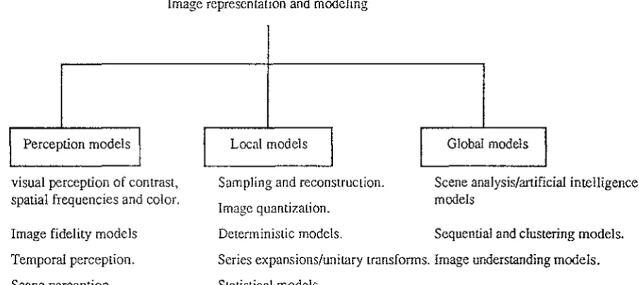
* Image representation and modelling

[image:13.599.41.476.87.277.2]

two-dimensional function that bears information can be considered an image. Image models give a logical or quantitative description of the properties of this function. Figure 1-2 lists several image representation and modelling problems.

Image representation and modeling

Perception models

visual perception of contrast, spatial frequencies and color.

Image fidelity models

Temporal perception.

Scene perception.

Local models

Sampling and reconstruction.

Image quantization.

Deterministic models.

Global models

Scene analysis/artificial intelligence models

Sequential and clustering models.

Series expansions/unitary transforms. Image understanding models.

Statistical models.

Fig. 1-2 Image representation and modelling * Image enhancement

In image enhancement, the goal is to accentuate certain image features for subsequent analysis or for image display. Examples includes contrast and edge enhancement, pseudocoloring, noise filtering, sharpening, and magnifying. Image enhancement is useful in feature extraction, image analysis, and visual information display. The enhancement process itself does not increase the inherent information content in the data. It simply emphasises certain specified image characteristics. Enhancement algorithms are generally interactive and application-dependent.

* Image restoration

[image:14.597.51.504.144.346.2]

of a sensor or its environment, noise filtering, and correction of geometric distortion or nonlinearities due to sensors.

* Image analysis

Image analysis is concerned with making quantitative measurements from an image to produce a description of it. In the simplest form, this task could be reading a label on a grocery item, sorting different parts on an assembly line, or measuring the size and orientation of blood cells in a medical image. More advanced image analysis systems measure quantitative information and use it to make a sophisticated decision, such as controlling the arm of a robot to move an object after identifying it or navigating an aircraft with the aid of images acquired along its trajectory.

Image analysis techniques require extraction of certain features that aid in the identification of the object. Segmentation techniques are used to isolate the desired object from the scene so that measurements can be made on it subsequently. Quantitative measurements of object features allow classification and description of the image.

* Image data compression

The amount of data associated with visual information is so large (see Table

applications, data compression 1s of great importance 1n digital image processing.

Table l.la Data Volumes of Image Sources (in Millions of Bytes) National archives

1 h of colour television Encyclopaedia Britannica

Book (200 pages of text characters) One page viewed as an image

Table 1.lb Storage Capacities (in Millions ofBytes) Human brain

Magnetic cartridge Optical disc memory Magnetic disc

2400-ft magnetic tape Floppy disc

Solid-state memory modules * Image reconstruction from projections

12.5x 109

28x 103

12.5x 103

1.3

0.13

125,000,000 250,000 12,500

760

200

1.25 0.25

P.~onttruction '

-algorithm

<!I

_I

:k

'

,,

---·L...l.~----.,.-

_----r,

.Xnyi

~~-,----t

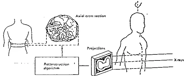
l

Fig. 1-3 Image reconstruction using x-ray CT scanners. 1.2. The Fundamentals of Computerized Tomography

We know that x- rays, radioisotopes, ultrasound and magnetic resonance can be used to obtain a reconstructed image. Because x-rays are broadly used today, we will only discuss utilizing x-rays to form the images based on their attenuation coefficient.

On November 1895, Professor Rontgen discovered the x-rays. The prospects for x-ray diagnosis were immediately recognised. In Great Britain, it has been estimated that there are 644 medical and dental radiography examinations per 1000 population per year, so that the technique is of major importance in medical imaging.

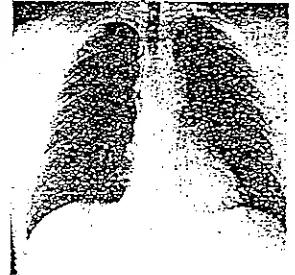
[image:17.596.114.434.75.207.2]

[image:18.597.168.316.168.306.2]

When we look at a chest x-ray (see Figure 1-4), certain anatomical features are immediately apparent. The ribs, for example, show up as a light structure because they attenuate the x-ray beam more strongly than the surrounding soft tissue, so the film receives less exposure in the shadow of the bone. Correspondingly, the air-filled lungs show up as darker regions.

Fig. 1-4 Typical chest x-ray radiograph

X-ray films usually allow contrasts of the order of 2% to be seen easily, so a 1 cm thick rib or a 1 cm diameter air-filled trachea can be visualised. However, the blood in the blood vessels and other soft-tissue details, such as details of the heart anatomy, cannot be seen on a conventional radiograph. In order to make the blood vessels visible, the blood has to be infiltrated with a liquid contrast medium containing iodine compounds; the iodine temporarily increases the linear attenuation coefficient of the fluid medium to the point where visual contrast is generated. Consideration of photon scatter further degrades contrast.

Another problem with the conventional radiograph is the loss of depth information. The three-dimensional structure of the body has been collapsed, or projected, onto a two-dimensional film.

It is apparent that conventional x-radiographs are inadequate in these two respects, namely the inability to distinguish soft tissue and the inability to resolve spatially structures along the direction of x-ray propagation.

Institute of Radiology annual conference, has been described as the greatest step forward in radiology since Rontgen's discovery. The relevant abstract (Ambrose and Hounsfield 1972) together with the announcement entitled 'X-ray diagnosis peers inside the brain' in the New Scientist (27 April 1972) can be regarded as the foundation of clinical x-ray CT. Hounsfield shared the 1979 Nobel Prize for Physiology and Medicine with Cormack.

With computerized tomography, the two inabilities of conventional x-radiographs can be solved. By combining "ordinary" x-ray technology with sophisticated computer signal processing, computerized tomography can generate a display of the tissues of the body which is unencumbered by the shadows of other organs. Computerized tomography also passes x-rays through the body of a patient, but the detection method is usually electronic in nature, and the data is then converted from an analogue signal to digital impulses in an analogue-to-digital (A/D) converter. This digital representation of the x-ray intensity is fed into a computer, which then reconstructs an image.

Since Hounsfield's invention of the computerized tomography (CT) scanner in 1972, great improvements have been made in x-ray tomography, with the result that the patient scan time has been reduced to less than 10s from over 4 m1ns.

1.2.1. Theoretical Background for Image Reconstruction

1.2.1.1. The N-Dimensional Continuous Fourier Transform (CFT)

We consider here a function _{f(xpx2, ... ,xN)} of N continuous variables

Xi,X₂, ••• ,xN. We will generally find it convenient to express the N-tuple

+oo +oo

F(mpm2, ... , mN)

=

J ... J

f(xi,x2, ... ,xN )exp[-_j(m1x1

+

_{m2x2+ ... +mNxN )]dx1dx2 ... dxN}

or, expressed in vector notation,

and

+oo

F(iiJ)=

f

J(x)exp[-J(.x•w)]dx

f(x)

=

l

NT

F(m)exp[j(.x · w)]dm

(2n) _-oo

(1.1)

(1.2)

(1.3)

(1.4)

where

.x •

iiJ denotes the dot product of the vectors

x

and

w

or equivalently with

.x

and

m

interpreted as row matrices .x ·

m

=

.xw'.

A useful property of the N-dimensional Fourier transform pair which we will want to use later is that if f(x) and F(m) form a Fourier transform pair, then f(xA) and F(wA) form a Fourier transform pair if A is an orthogonal

t .

.

A-I A--1 ma nx, 1.e.,

=

.

This property is easily verified by direct substitution into (1.3). Thus an orthogonal transformation or equivalently an orthogonal change of coordinates in signal space results in the same change of coordinates in Fourier space. For example, for N=2, if

[

cose

sine]

A=

so that JCi) is rotated by an angle 0, then its Fourier transform will be rotated by the same angle 0.

1.2.1.2. The N-Dimensional Discrete Fornier Transform (DFT)

We are here interested in functions which can be processed by a digital computer and consequently can be represented by their samples. Thus we consider the class of band-limited functions. Specifically, JCi) is said to be band-limited if there exists an N-tuple (Wi,W_{2 , •••} ,WN) such that F(m) is zero

for

lm;I

> Wi> i

=

1,2, ... ,N. In some cases it is convenient to set

W

=

max(Wi, W_{2 , ••• ,} WN) and refer to the scalar Was the bandwidth of f(x). The N-dimensional sampling theorem states that if f(x) is sampled in signal space on a rectangular lattice with the sample spacing in dimension X; less

than TC I Wi, then f (x) can be recovered from its samples. Sampling on a

rectangular lattice will be referred to as periodic Cartesian sampling.

Let us denote by g(n) the N-dimensional sequence corresponding to sampling

f (x) with a sample spacing of TC I Vi in the dimension xi where Vi > Wi so that

(1.6)

from the sampling theorem the Fourier transform F(m) of f(x) can be obtained from g(n) by the relation

(1.7)

h - d h ( co1 CO2 wN ) d

w ere COv enotes t e vector - , - , ... , - an

v1 v2

vN

b y(CO) --{ 1,

lmil<Vi,

i=l,2, ... ,N

0, otherwise

+V

g(n)

=

l N

f

F(w)exp{jn(n · Q)y )}dw (27r) -V

(1.8)

The original N-dimensional function f(x) can be obtained from the sequence g(n) by means of the interpolation formula

where

+oo

f(x)

=

I:gCn)</JCn,x)

n=-oo

sin V. (x. - nin)

</J(n,x)

=

IT . .

vi

i=l V.(x.-nin)

l l

v.

l

(1.9)

(1.10)

When only a finite number of the samples of f(x) are nonzero, the Fourier transform F(w) can be represented by a finite set of Cartesian samples. The relationship between the Cartesian samples of F(w) and the Cartesian samples of f(x) is the N-dimensional DFT. Specifically, let us assume that

g(n) = 0, if ni ~ Mi or ni < 0, i = 1,2, ... ,N.

We now consider the Cartesian samples of F(w), which we denote by G(k)

given by

where k; is an integer such that

M. M.

-1

+

1 ~ ki ~ - 1

, if M; is even

2 2

- Mi - l < k. < Mi - l if M 1

. is odd

Then

and

( ) - 1 ~ ~Gk~ . ~~ ~~

4~

g

n,,,~, ...

,nN - - - L . , ; · · · L . , ; ( i,"'2,···,kN)•exp[J2n(-+-+ ... + - - ) ]

M1 ·Mz · ... ·MN k1 k2 M1 Mz MN

(1.12) Since G(ki,k_{2 , •••} ,kN) as defined in (1.11) is periodic in k; it is frequently convenient to use the values of k; in the range given above. Adopting this convention and defining the vector kM as the N-tuple

we can express (1.11) and (1.12) as M-1

G(k)

=

L

g(n) · exp[-j2n(n · kM )] (1.13)

n=O

and

(1.14)

The class of functions f (x) which can be represented by a finite number of samples will be referred to as band-limited functions of finite order M where

1.2.1.3. Projections

A projection is a mapping of an N-dimensional function to an (N-1)-dimensional function obtained by integrating the function in a particular direction. For example, Px

2 (x1) given by

+=

px₂ (x,)

=

f

_f(Xi,X2)dx₂ (1.15)

is an example of a projection of the two-dimensional function _f(xi,x2) onto one dimension.

For the general case, we define a projection as follows: Let f(x) denote an N-dimensional function and let i1 denote a new set of coordinates where

x=ilA

and A is an orthogonal transformation. Then a projection onto the hyperplane (upu2, ... ,u;_pu;+i,···,uN) is defined as

+=

Pu; (llpU2,···,Ll;_pU;+i, ... ,uN)

=

I

f(uA)du; (1.16)

The coordinate axis u;, which is normal to the hyperplane onto which f(x) is projected, will be referred to as the projection axis.

For N =2, the matrix A is given by

[

cos

e

sine] A=

In this case, the Ui, Uz coordinate axes are offset from the (x1,x2 ) axes by an

angle of 0. For two-dimensional functions it will generally be convenient to

refer to a projection by its angle 0. A projection at angle 0 will be interpreted

to mean a projection onto the coordinate ½, which is at an angle 0 with x₁•

Equivalently, then, the projection axis Uz is at an angle 0 to the coordinate axis x_{2 •} Equation (1.15) corresponds to a projection at an angle 0

=

0 or equivalently with x2 as the projection axis.

1.2.1.4. The Projection-Slice Theorem

The projection-slice theorem relates the (N-1)-dimensional Fourier transforms of the projections to the N-dimensional Fourier transform of the original function. Basically, the theorem states that the (N-1)-dimensional Fourier transform of a projection is a "slice" through the N-dimensional Fourier transform of f (x).

First, let us consider a projection for which the projection axis is one of the coordinate axes of f(x), for example, x_{1 •} Then px

1 (x2 , ••• ,xN) is given by

+=

Pxl (Xz,···,XN)

=

f

f(x)dx1 (1.17)

and its (N-1)-dimensional Fourier transform is given by

+oo +oo

Px, (OJz,···, (J)N)

=

J ...

f

Px, (Xz,···,XN). exp[-j(OJ2X2+ ... +WNXN )] (1.18)

Comparing (1.18) and (1.1), we see that

(1.19)

In other words, Px

1 (OJ2 , ... ,0JN) is a "slice" of F(wpw2, ... ,wN) defined by OJ1 =0.

A general projection was defined in (1.16) where A is an orthogonal transformation. It was argued previously that if F(w) is the Fourier transform of f(x) then F(Q) is the Fourier transform of /(u) where

(1.20)

From this, (19) is easily generalized to state that a projection for which the projection axis is the transformed coordinate ui has an (N-1)-dimensional Fourier transform which is a slice of F(Q) for Qi

=

0 where the coordinate systems

u

and Q are related to the coordinate systems

x

and

m

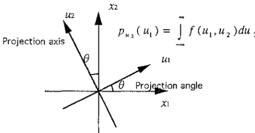
by the same orthogonal transformation. In two dimensions, for example, the projection-slice theorem states that the one-dimensional Fourier transform of a projection at an angle 0 is a slice at the same angle of the two-dimensional Fourier transform of the original object. This relationship is depicted in Figure 1-5.

X2

U2

Projection axis

[image:26.599.121.384.364.501.2]

(I) 2

Fig. 1-5 The relationship between the projection of a two-dimensional function and slice of its Fourier transform.

1.2.1.5. The Basis for Reconstruction from Projections

From the projection-slice theorem, we see that specification of a projection in signal space corresponds to the specification of a slice in Fourier space and thus represents a partial specification of the signal itself. In principle, then, if an unlimited number of projections at different orientations are available, the Fourier transform of f(x) can be obtained and therefore so can f(x) itself. Generally, in any practical context, we are restricted to a finite number of projections.

Under certain assumptions, it is possible to carry out an exact reconstruction from a finite number of projections. If the structure is highly symmetrical, a finite number of projections might suffice for exact reconstruction. For example, for a two-dimensional circularly symmetric function all of its projections are identical and consequently such a function can be represented exactly by a single projection. Similarly, in three dimensions, for an object which is cylindrically symmetric all of the projections for which the axis is normal to the longitudinal axis are identical and consequently, in this case also, a single projection is sufficient.

[image:27.597.185.380.62.205.2]

of each projection is a function of a set of continuous variables, but only a finite number of points from each Fourier transform can be computed and stored. Thus from the projections, only samples in the Fourier domain are available, in part because of the limited number of projections and in part because only samples of the Fourier transform on each slice can be obtained. The essence of the reconstruction problem, then, is to approximate all of Fourier space from its values on a discrete point set.

1.2.1.6. Reduction of the Dimensionality of the Reconstruction Problem

As we saw in Section 4, the underlying basis for reconstruction is to obtain samples in the Fourier plane by transforming projections. Intuitively it seems reasonable that projections need not be taken in all orientations. For three-dimensional objects, for example, we could imagine using only projections in the spatial domain on planes parallel to one of the coordinates axis, say x1 • Slices of these projections at x1

=

A are then projections of the

two-dimensional function f(A,x₂,xJ and, consequently, a two-dimensional reconstruction algorithm can be applied to reconstructing this two-dimensional slice of the two-dimensional object. In this way, the dimensional object can be built up slice by slice and, consequently, the three-dimensional problem can be reduced to a series of two-three-dimensional problems. In the general case, we can apply a similar argument to reduce an N-dimensional problem to a set of (N-1)-dimensional problems each of which can in principle be reduced to an (N-2)-dimensional problem, etc.

CHAPTER 2. INTRODUCTION TO PARALLEL PROCESSING AND TRANSPUTERS

2.1. The Principles of Parallel Processing Systems

In real life, things occur in parallel. Consider how unrealistic it would be if that were not the case.

It would be most strange if, whilst waiting for a roll of

film to be developed at the printer, the photographer did not continue to take photographs, assuming both film and camera were available and operative. The manager who needs to present information in a meaningful way, does not wait until a report has been typed before undertaking any further work. To be efficient, these tasks must be carried out in parallel.

The reasons for finding the parallel method of operation preferable to the sequential mode are quite apparent. The sequential mode leads to a very uneconomical time management function, being a tremendous waste of time and resources.

It is the same that a simple-minded approach to gain speed, as well as power, in computing is through parallelism; here many computers would work together, all simultaneously executing some portions of a procedure used for solving a problem. Such an approach rests on the following assumptions:

(1) The availability of many low-cost, high speed computers that can be put together to work in unison, as in a concert;

(2) the existence of a strategy to partition a problem into smaller problems, such that most of these can be solved simultaneously, and from which we can easily construct the solution to the entire problem: this is popularly known as the "divide-and-conquer strategy".

fabricate millions of transistor-equivalent devices on a single 4mm square silicon ship. Several hundreds of thousands of such chips can be put together to build several thousands of processors within a few cubic centimetres at a reasonable cost.

The second of these assumptions, namely the application of the divide-and-conquer strategy, raises three basic issues:

(1) decomposability, (2) complexity, and (3) communication.

We shall consider these issues below. Decomposability.

Decomposibility is a measure of the degree by which a problem can be split into components which can be computed in parallel. Some problems appear to be inherently serial in nature and not amenable to parallel processing. It is however not easy to determine whether a problem is inherently serial as it is often possible to reformulate problems into a form suitable for parallel processing.

A very simple example is the sum of a set of figures. This appears to be an inherently serial problem. However if we reformulate the problem in a hierachical form, the addition of pairs of numbers may be partially computed in parallel.

e.g .. A=l,2,5,7,9

1+2

"'

/

+

_'

5+7

_► s

/

+

9

Fig. 2-1. Diagram to show that two summation can be performed in parallel Complexity.

As mentioned before, to obtain the maximum gain 1n speed, several processors should be used to process the decomposed tasks. The effectiveness of this depends on how well a problem can be partitioned for solution by a given computer architecture or by an algorithm.

For instance, let T be the total time taken by an algorithm in which there is a serial portion taking time Ts and a parallel portion taking time TP, so that Ts+ TP

=

T; then, no matter how many processors are used, the serial portion would limit the increase in speed by a factor of at most T / Ts; this is because at best TP can go down to near zero! Thus, if an algorithm has a 10% serial portion, the speed increase that can be achieved by putting infinitely many processors to work would still be limited to ten times.

Therefore a judicious choice is needed in partitioning an algorithm and minimizing the serial portion.

Communication.

[image:31.597.163.388.64.192.2]

links between any two tasks among n tasks could be n(n-1) and so the communication complexity grows quadratically. The communication problem introduces a new dimension to parallel programming and parallel architecture design. This means that in addition to the computing time and memory space requirements of an algorithm, we must also consider the communication costs and set a bound on the complexity of communication. This would imply that communication between tasks which are not close enough (closeness being measured by a suitably defined criterion for an architecture) should be avoided; that is, the communication should preferably be confined to only those processes that are very close neighbours. When a large number of processors are assigned to carry out the split tasks, it is possible that simultaneous request or access to certain data or tasks may create a conflict or collision. This could slow down the anticipated speed advantage resulting from the multiple processors, or may even lead to a state of inactivity or standstill when two processes or processors wait for each other indefinitely (deadlock), or may delay some process indefinitely (lockout). Since the computational speeds for different tasks are unpredictable (non-deterministic), the different processes may loss synchronisation, leading to a total breakdown of the tasks.

The communication problem is therefore concerned with the minimisation of communication complexity, prevention of deadlocks and improved coordination.

In recent years, the models and techniques employed to solve the three basic issues, namely decomposability, complexity and communication, have grown into a major interdisciplinary science of parallel processing. This science deals with both the theoretical studies and the practical aspects of design to achieve the best results.

2.2. Description of Parallel Processes

of operations. Therefore, a sequential program is easily described with the help of flow diagrams containing the following well-known deterministic constructs (or boxes):

(1) begin (start); (2) assignment (set);

(3) if B then S else T (decision); (4) while B do S (indefinite loop); (5) for i=l ton (definite loop); (6) end (halt).

In the case of parallel or non-sequential programs, in addition to the above constructs we need the following mechanisms:

(1) parallel initiation and termination mechanisms;

(2) synchronisation, protection and communication mechanisms; 2.2.1. Initiation and Termination Mechanisms

When a set of processes are non-sequential we need to have constructs that can begin a list of processes simultaneously and end a list of processes when all of them terminate. These are respectively called cobegin and coend constructs.

2.2.2. Synchronization Mechanism

2.2.3. Protection Mechanism

The synchronisation mechanism alone is not adequate to carry out non-sequential programming. In order to coordinate the processes it is also necessary to prevent clashes among them. That is, we must restrict the access of a shared variable or a resource to one process at a time. This is achieved by using another mechanism called the protection mechanism. This protection mechanism prevents interference or clashes from other processes when a particular process is using a shared variable or a resource.

The sequence of statements in which access to a shared variable or resource is to be exclusively provided to a process is called a critical section or critical region. When a process is about to execute its critical section we avoid a clash by ensuring that no other process is executing its own critical region at the same time. Then once access is given to a process, access by another process should be allowed by an unlocking process. In other words, the protection mechanism should provide a locking facility to allow each process to perform its critical section and to unlock and let the other processes do their own critical sections.

2.2.4. Communication Mechanism

Two distinctly different methods are used for synchronisation among processes.

(1) Shared-variable method.

In this method, synchronisation and communication among the processes are achieved using shared mechanisms under a centralised control.

(2) Message-passing method.

delay and wait operations among them. These two methods have contributed to the development of new styles of programming languages for concurrent programming.

The design of methods for the description of parallel processes and the synchronisation and protection mechanisms has been a very active area of research during recent years. As a result of these studies, new concepts and analytic models have been developed for the programming, complexity and analysis of parallel and concurrent processes.

2.3. The Transputer

The transputer comprises a single chip, made using very large scale integration (VLSI) techniques which condense the equivalent of 250,000 transistors onto a chip measuring 9mm square. Some of the transputer's circuitry and elements are as small as 1.5 micrometers.

The objective of the transputer is to generate high performance calculations and currently, the most powerful transputer can process 10 million program instructions per second. This is faster than any other 32-bit microprocessor and has the advantage of being increased when working in conjunction with other transputers.

The transputer does not operate using a series of sequential steps, but is a parallel processor with the ability to carry out several computations simultaneously. The management of this parallel facility may be carried out via the purpose-built concurrent programming language Occam.

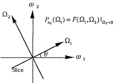
2.3.1.0verview

RESET

_{- - - ~}

ANALYSE _---,....-J

ERROR

Boot from ROM

- - - - 1 ~

vcc

_{- - - ~}

GND

----,....-J

SYSTEM SERVICES

ON-CHIP

RAM APPLICATION

SPECIFIC INTERFACES

PROCESSOR

[image:36.597.53.505.52.310.2]

LINK INTERFACE

Fig. 2-2 Block diagram of the transputer

LINK IN

LINK OUT

The transputer has been specifically developed for concurrent processing. The on-chip local memory assists in eliminating processor-to-memory bottlenecks, and each transputer supports 4 asynchronous, high speed serial links to other transputer units. The efficient utilisation of each processor's time slices is carried out by a microcoded scheduler.

The transputer-to-transputer links provide a combined data communications capacity of 5 Megabytes/sec and operate concurrently with internal processes. This is a radical departure from the shared bus concept employed in the majority of multiprocessor architectures.

It

allows parallel connection without the overhead resulting from having to provide the complex communications between conventional parallel processors. The advantages over multi-processor buses are as follows:

- No contention for communications

- No capacity load penalty as transputers are added

The system architecture may comprise either a single transputer chip or a network of transputers functioning together as a concurrent system.

Low cost systems which perform at supercomputer speeds are quite easily achieved. This is because when transputers are connected together there is an increase in processing power available which, as there is no communication overhead, theoretically has no limit.

2.3.2. Occam

The system supports a high level concurrent programming language, Occam, specifically designed to run efficiently on transputer systems. Occam allows access to machine features and removes the need for a low level assembly language.

Occam and the transputer were designed together enabling optimal implementations of Occam to be achieved with respect to concurrency and communications. The transputer instruction sets have been designed for efficient and simple Occam compilation.

An Occam program comprises a set of sequential or parallel processes, or may comprise a number of other processes.

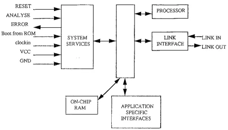
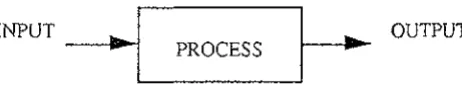
There are three primitive processes upon which all else is based, these being assignment , input and output.

INPUT _----,►~

I

_PROCESS 1---1111►► OUTPUT

Fig. 2-3. Processes of a transputer

An assignment changes the value of a variable, an input receives a value from a channel, and an output sends a value to a channel.

[image:37.597.159.390.523.566.2]

v:=e

sets the value of the variable v to the value of the expression e and then terminates.

An input is indicated by the symbol ? The example

c?x

inputs a value from channel c, assigns it to the variable x and then terminates.

An output is indicated by the symbol ! The example c!e

outputs the value of the expression e to channel c.

Sequential programming languages deal with processes as a number of statements to be executed strictly in sequence. In the real world, just as a large, work intensive task would be split between many people in order to utilise the available workforce and to improve performance levels, so a process can be expressed in terms of modules which may be executed concurrently. The Occam language enables an application to be expressed in terms of a number of concurrent processes which communicate using channels.

For example, Occam can express an application as follows: PAR

The component processes Pl, P2, P3 ... are executed together, and are called concurrent processes. The construct terminates after all of the component processes have terminated, for example:

PAR

cl? x c2 ! y

allows the communications on channels cl and c2 to take place together. The parallel construct is unique to OCCAM. It provides a straightforward way of writing programs which directly reflects the concurrency inherent in real systems.

Occam can be applied to a system with one transputer or one which is made up of many transputers. A program written in Occam may be implemented on a single transputer, or, without modification, (although some modification may enhance performance) it may be implemented on a system with more than one transputer. In this situation each transputer would be executing an Occam process, and the links between the transputers would provide the Occam channels. Occam may be used as a design language for such a system, describing both the system as a whole, as well as each individual transputer.

OCCAM programs may be configured for execution on one or many transputers. The transputer development system provides the necessary tools for correctly distributing a program configured for many transputers. Configuration does not affect the logical behaviour of a program. However, it does enable the program to be arranged to ensure that performance requirements are met.

PLACEDPAR

1s executed by a separate transputer. The variables and times used in a placement must be declared within each placement process.

PRIPAR

On any individual transputer, the outermost parallel construct may be configured to prioritise its components. Each process is executed at a separate priority. The first process has the highest priority, the last process has the lowest priority. Lower priority components may only proceed when all higher priority components are unable to proceed.

2.3.3. Communication Channels

Two processes or equivalently, two transputers, communicate via channels. These channels are one-way with one process writing to the channel and the other process reading from the channel. When it is required that communications between processes takes place, the two processes must synchronise, that is, they must both be ready. If necessary, one process must wait for the other.

Two processes communicating is equivalent to two transputers communicating; this mode of communication is similar to the handshake method used in hardware systems.

Internally, there may be many concurrently performing communications channels because Occam may be used for a single transputer or a whole network of maybe thousands. If the system comprises a single transputer then the processor time is shared between the concurrent processes with channels being achieved by a block movement of data in memory.

Concurrent processes communication only by using channels, and communication is synchronized. If a channel is used for input in one process, and output in another, communication takes place when both the inputting and the outputting processes are ready. The value to be output is copied from the outputting process to the inputting process, and the processes then proceed.

CHAPTER 3. RECONSTRUCTION ALGORITHMS FOR PARALLEL AND FAN BEAM PROJECTIONS

The projection slice theorem [5] relates the Fourier transform of a projection to the Fourier transform of the object along a single radial. Thus given the Fourier transform of a projection at enough angles the projections could be assembled into a complete estimate of the two-dimensional transform and then simply inverted to arrive at an estimate of the object, while this provides a simple conceptual model of tomography, practical implementations require a different approach.

The algorithm that is currently being used in almost all applications of straight ray tomography is the filtered backprojection algorithm. It has been shown to produce accurate reconstructions and amenable to fast implementation, it is derived from the Projection Slice Theorem. This theorem is brought into play by rewriting the inverse Fourier transform in polar coordinates and rearranging the limits of the integration therein. The derivation of this algorithm is perhaps one of the most illustrative examples of how we can obtain a radically different computer implementation by simply rewriting the fundamental expressions for the underlying theory. In this chapter, details will be presented for the filtered backprojection algorithms for two types of scanning geometries, parallel beam and fan beam. Then, a modified reconstruction algorithm will be advanced, it reduces the computational requirements of backprojection. The computer implementation of these algorithms requires the projection data to be sampled and then filtered. We will first provide an intuitive rationale behind the filtered backprojection approach.

3.1 Reconstruction Algorithm for Parallel Projections

3.1.1. The Idea

Fourier transform is found of the projection at each angle then it follows easily by the Projection Slice Theorem [5]. We say that the projections are nearly independent (in a loose intuitive sense) because the only common information in the Fourier transforms of the two projections at different angles is the de term.

To develop the idea behind the filtered backprojection algorithm, we note that because of the Fourier Slice Theorem the act of measuring a projection can be seen as performing a two-dimensional filtering operation. Consider a single projection and its Fourier transform. By the Fourier Slice Theorem, this projection gives the values of the object's two-dimensional Fourier transform along a single line. If the values of the Fourier transform of this projection are inserted into their proper place in the object's two-dimensional Fourier domain then a simple (albeit very distorted) reconstruction can be formed by assuming the other projections to be zero and finding the two-dimensional inverse Fourier transform. The point of this exercise is to show that the reconstruction so formed is equivalent to the original object's Fourier transform multiplied by the simple filter shown in Figure 3-1.

I•) (hi (<J

Fig. 3-1 Filter process

This figure shows the frequency domain data available from one projection. (a) is the ideal situation. A reconstruction could be formed by simply summing the reconstruction from each angle until the entire frequency domain is filled. What is actually measured is shown in (b). As predicted by the Fourier Slice Theorem, a projection gives information about the Fourier transform of the object along a single line. The filtered backprojection algorithm takes the data in (b) and applies a weighting in the frequency domain so that the data in (c) are an approximation to those in (a).

It is important to remember that this summation can be done in either the

Fourier domain or in the space domain because of the Fourier transform. As will be seen later, when the summation is carried out in the space domain, this constitutes the backprojection process.

As the name implies, there are two steps to the filtered backprojection algorithm: The filtering part, which can be visualized as a simple weighting of each projection in the frequency domain, and the backprojection part, which is equivalent to finding the elemental reconstructions corresponding to each wedge filter mentioned above.

The first step mentioned above accomplishes the following: A simple weighting in the frequency domain is used to take each projection and estimate a pie-shaped wedge of the object's Fourier transform. Perhaps the simplest way to do this is to take the value of the Fourier transform of the projection, s₈(w), and multiply it by the width of the wedge at that frequency. Thus if there are K projections over 180° then at a given frequency w, each wedge has a width of 21elwl / K.

The effect of this weighting by 21elwl/ K is shown in Figure 3-l(c). Comparing this to that shown in (a) we see that at each spatial frequency,

w,

the weighted projection, (21elwl I K)s₀(w), has the same "mass" as the pie-shaped wedge. Thus the weighted projections represent an approximation to the pie shaped wedge but the error can be made as small as desired by using enough projections.

The final reconstruction is found by adding together the two-dimensional inverse Fourier transform of each weighted projection. Because each projection only gives the values of the Fourier transform along a single line, this inversion can be performed very quickly. This step is commonly called a backprojection since, it can be perceived as the smearing of each filtered projection over the image plane.

*

Measure the projection, P0(t)

* Fourier transform it to find s₀(co)

* Multiply it by the weighting function 2rclcol / K

* Sum over the image plane the inverse Fourier transforms of the filtered projections (the backprojection process).

There are two advantages to the filtered backprojection algorithm over a frequency domain interpolation scheme. Most importantly, the reconstruction procedure can be started as soon as the first projection has been measured. This can speed up the reconstruction procedure and reduce the amount of data that must be stored at any one time. To appreciate the second advantage, it should be noted that in the filtered backprojection algorithm, when we compute the contribution of each filtered projection to an image point, interpolation is often necessary; it turns out that it is usually more accurate to carry out interpolation in the space domain, as part of the backprojection or smearing process, than in the frequency domain. Simple linear interpolation is often adequate for the backprojection algorithm while more complicated approaches are needed for direct Fourier domain interpolation.

3.1.2. Theory

The derivation of the backprojection algorithm for a parallel beam geometry begins with the inverse Fourier transform: [7]

+e.o+oo

f(x,y)=

I

fFCu,v)ejZ1t(ux+vy)dudv

(3.1)

Converting to polar coordinates and substituting the Fourier transform of the projection at angle 0, s₉(co), for the two-dimensional Fourier transform F(co,0), we get

where

;t

f(x,y)=

f

Q₀(xcos0+ysin0)d0

0

+=

Q0(t) =

J

s8(CD)lwlej

2_{=tdw (3.3)}

This estimate of ftx,y), given the projection data transform se(m), has a simple form. Equation (3.3) represents a filtering operation, where the frequency response of the filter is given by 1ml; therefore Q₀(t) is called a "filtered projection." The resulting projections for different angles 0 are then added to form the estimate of f(x,y).

Equation (3.2) calls for each filtered projection, Q₀, to be "backprojected."

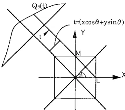
This can be explained as follows. To every point (x,y) in the image plane there corresponds a value of t = xcos 0 + ysin 0 for a given value of 0 , and the filtered projection Q₀ contributes to the reconstruction its value at t (=xcos0+ysin0). This is further illustrated in Figure 3-2. It is easily shown that for the indicated angle 0 , the value of t is the same for all (x,y) on the line LM. Therefore, the filtered projection, Q₀, will make the same

contribution to the reconstruction at all of these points. Therefore, one could say that in the reconstruction process each filtered projection, Q₀, is

smeared back, or backprojected, over the image plane.

[image:46.599.140.357.429.620.2]

t=(xcos0i+ysin0i) y

f

+W . 2W N/2 2W

I

2w1 j21tm(2w )t Qe(t)= se(co)lcoleJ2_{1\'.ll)tdw = -}

L

_s

0( m - ) m - e N

-W N m=-N/2 N N

(3.4)

where the frequency domain is assumed bandlimited and the projection data is assumed to be zero for large values of It I.

However the requirement of finite order and finite bandwidth will lead to artifacts in the reconstructed image. The artifacts can be eliminated by the following alternative implementation of (3.3) which doesn't require the approximation used in the discrete representation of (3.4). When the highest frequency in the projections is finite, (3.3) may be expressed as

where

where, again,

{

1 !col <W bw(co)

=

0

otherwise

(3.5)

(3.6)

-1/2,z 1/2,z Frequency(w)_....,_

Fig. 3-3 The ideal filter response for the filtered backprojection algorithm is shown here. It has been bandlimited to 1 / 2 r.

H(m), shown in Figure 3-3, represents the transfer function of a filter with which the projections must be processed. The samples of impulse response,

h(nr), of this filter is given by the inverse Fourier transform of H(m) and is

1/ 4"C2, n

=

0

h(n"C)

=

0, n even

1

2 2 2, n odd

n n 'C

This function is shown in Figure 3-4.

[image:48.597.130.404.56.258.2]

h(nr) 1/4~

I \

I \

I \

I \

\ I

V

-l/mr2

Fig. 3-4 The impulse response of the filter shown in Fig. 3-3

Since both P0(t) and h(t) are now bandlimited functions, they may be expressed as

P/t)=

t

Pe(kt)sin2rcW(t-kr)

k=-= 2rcW(t-kr)

(3.9)

h(t) =

f

h(kc) sin2rcW(t-kc)

k=-= 2rcW(t-kr)

(3.10)

By the convolution theorem the filtered projection (3.5) can be written as

(3.11)

Substituting (3.9) and (3.10) in (3.11) we get the following result for the values of the filtered projection at the sampling points:

=

Q₀ (nt) = "C

I,

h(n"C - k1:)P₈ (k-r) (3.12)

[image:49.597.135.405.53.310.2]

In practice each projection is of only finite extent. Suppose that each P₈ (k1:) is zero outside the index range k=0, ... ,N-1. We may now write the following two equivalent forms of (3.12):

N-1

Q₀(n1:) = 'C I,h(n1:-k1:)P₈(k1:), n = 0,1,2, ... ,N -1 (3.13)

k=O

or

N-1

Q0(n1:)=1: I,h(k1:)P0(n1:-k1:), n=0,1,2, ... ,N-1 (3.14)

k=-(N-1)

The discrete convolution in (3.13) or (3.14) may be implemented directly on a general purpose computer.

3.2. Reconstruction Algorithm for Fan Projections

,,

Fig. 3-5. A fan beam projection is collected if all the rays meet in one location. According to the [7], The final equation for fan beam geometry to reconstruct

.

.

an image 1s:

112;,; 1 '

f(r,<j>)

= -

-

₂ Q (y )d~ 2

°

L p

(3.15)

where

(3.16)

and where

[image:51.596.143.389.97.370.2]

Here

p

is the angle that the source S makes with a reference axis, and angle y gives the location of a ray within a fan, and Dis the distance of the source S from the origin O.

This calls for reconstructing an image using the following three steps:

Step 1:

Assume that each projection Rp(y) is sampled with sampling interval a. The known data are then Rpi (na) where n takes integer values and

Pi

are the angles at which projections are taken. The first step is to generate for each fan projection Rpi (na) the corresponding R'pi (na) by

(3.18)

Note that n=O corresponds to the ray passing through the center of the projection.

Step 2:

Convolve each modified projection R'.o; (na) with g(na) to generate the corresponding filtered projection:

(3.19)

Step 3:

(a)

(bl

Fig. 3-6. Fan and parallel beam projections.

While the filtered projections are backprojected along parallel lines for the parallel beam case (a), for the fan beam case the backprojection is performed along converging lines (b).

[image:53.596.145.376.115.571.2]

From the presentation, it is obvious that the reconstruction algorithm for fan beam projection is similar to the parallel projection, so we will only consider the parallel projection.

3.3. Modified Back.projection Algorithm

From section 3.1, we know that the standard reconstruction equations are 1 2n oo

f(x,y)=-

J

JQ(0,t)•o(xcos0+ysin0-t)dtd0

2 0 -oo

00

Q(0, t) = JP(0,a)g(t-a)da

-oo

(3.20)

(3.21)

Equation (3.21) convolves the parallel projection P with an anti-blurring kernel g and equation (3.20) performs the backprojection of the filtered projection Q over the reconstruction area f using the mapping function 8. The name mapping function is adopted because it maps the projection functions onto the reconstruction area.

The measurement hardware provides a finite number of projections N at equi-angular displacements around the object, each containing M rays, and the reconstruction area is divided up into an array of rectangular pixels (Cartesian pixel geometry). Incorporating these into equation (3.20) gives the discrete backprojection equation

1N-l M

f(L:ix,k~y) = -

I, I,

Q(nt-.0,m~t)o(lt..xcos(nt..0) + Mysin(nt..0)-rnLit)

2 n=Om=-M

(3.22) where l=l,2,3, ... , L. k=l,2,3, ... , K.

function 8₁ may be nearest-neighbour, linear, or other more elaborate interpolation scheme. However linear and nearest-neighbour are the most common due to their low computational requirement.

An obvious implementation of equation (3.22) would be to pre-calculate the values of the mapping function and store them in a look-up table for subsequent retrieval at run-time. For the standard algorithm using nearest-neighbour interpolation, this requires N x W elements in the table (where N is the number of projections, and W is the number of pixels in the reconstruction area).

It is possible to reduce the size of the mapping function by a factor of N by discretising the reconstruction area using a non-Cartesian coodinate system. In order to develop an algorithm which will achieve this reduction, the coordinates of the standard backprojection equation (3.20) are transformed from Cartesian (x,y) to polar (r,¢).

1 2ir~

f(r,¢) =

2

ff

_o-~ Q(8, t)o(rcos[<P- 8]-t)dtd8 (3.23)

Equation (3.23) describes the system as continuous in both the reconstruction area and the projection space. However the projection space is discrete by

nature of the physical hardware in both the ray position t and the projection angle

e.

Thus equation (3.23) becomes

1 N-1 M

f(r,</>)=-I, I,Q(nLi8,mLit)8₁(rcos[¢-nLi8]-mLit) 2 n=Om=-M

(3.24)

An interpolating mapping function 8₁ is required because the filtered projection data is only available at discrete points, although the reconstruction space f is still described as continuous. The reconstruction area can be divided into N equal angular segments of size Li8 where Li8 is the angular displacement between projections. The angle </> in equation (3.24)

j = truncation(_!_), ¢' = modulo(¢,Li0) 1::,.0

Equation (3.24) becomes

, 1 N-1 M • •

f(r,jii8 + ¢) = -

I, I,

Q(nii0,miit)8/rcos[(J-n)!::,.0+ </> ]-miit)

2 n=Om=-M

(3.25)

(3.26)

Since (j-n)Li0 is azinuthally periodic it may be replaced by the expression module ((j-n),N)Li0, and by defining the mapping function for values j=O, ... , N-1 at one angle nLi0, the function 8₁ is defined for all projection angles

nii0, n=l, ... , N. The general modified backprojection equation is

, 1 N-1 M ,

f(r,jii0 + </>) = -

I, I,

Q(nt::,.0, miit)o₁ (rcos[mod[(j- n),N]t::,.0 + ¢ ]- miit) 2 n=Om=-M

(3.27) The mapping function 8₁ in equation (3.27) is reduced by a factor of N from equation (3.26).

To implement equation (3.27) using a digital computer it is necessary to discretise the reconstruction area f. Since most current tomographic systems require a large number of projections, the number of sectors in the reconstruction area will also be large (because the number of sectors is determined by the number of projections N).

It

is reasonable then to discretise the rotational component in equation (3. 75) from jii0 + ¢' to iii¢, where Li¢=

Lie

(as the segment angle is the same as the projection increment angle), and the radial component from r to (h- .!.)t::,.r where h is an integer

2

greater than zero. This pixel geometry is shown in Figure 3-11 and is described by

1 1 N-1 M 1

f([h- -]!::,.r,iii¢) = -

I, I,

Q(nii0,miit)8₁ ([h- -]!::,.rcos[(i-n)!::,.0]-miit)

[image:57.596.212.345.70.210.2]

Fig. 3-.7. Equi-Radia1/Angular Pixel Geometry

To arrange this reconstruction area onto a Cartesian array of elements appropriate for digital processing, we consider the radial component r in the x-direction, and the angular component </> in they direction. Equation (3.28)

can now be written 1 N-1 M

f(x,y) = -

I, I,

Q(n6.8,m6.t)8₁ (xcos(y-n6.8)- m6.t)

2 n=Om=-M

(3.29)

where x=l,2,3, ... , X; y=l,2,3, ... Y.

Using nearest-neighbour interpolation the mapping function is t

8_{1 (} t) = c5(rnd[-])

6.t (3.30)

where rnd indicates the mathematical rounding operation.

Let the mapping function 8₁ be defined for all points (x,y) in the first projection (n6.0 = 0). Noting that an x-directional shift in the exponential conformal (x,y) domain corresponds to a rotation in the (r, </>) domain about

To maximise the rate at which the algorithm can be processed, equation (3.29) must be broken down into small computational blocks which can all process information at the same time. In this form it is easy to implement on a systolic array, where each block makes up one element of the array.

The modified algorithm is well suited to pre-calculated table look-up techniques since the number of values in the mapping function are reduced by a factor of N (the number of projections), leaving the number of values equal to the number of pixels (Xx Y).

Defining the look-up table as y(x,y), equation (3.29) may be expressed as: 1 N-1 M

f(x,y)=-I LQ(nLi0,mLit)8₁(y(x,y)-~t)

2 n=Om=-M

(3.31)

By performing the round operation on the pre-calculated values, the argument in the mapping function will be integer, and mapping function 8₁ becomes the dirac function 8.

To separate the algorithm into a large number of cells suitable for systolic array organisation, each pixel (x,y) becomes an individual process. From equation (3.31) it is clear that each process involves selecting the correct value of Q corresponding to the appropriate y value. This value is then added to the pixel value. To implement this process each cell must contain:

(1) Storage for the image cell f(ex ,y)

(2) Storage for the filtered ray value Q(nLi8,mLit)

(3) Storage for the pre-calculated mapping function argument value y(x,y) ( 4) A counter m to increment the ray number ~ t