Fundamental aspects of quantum optics : a dissertation

Q U A N T U M O PTICS

A Dissertation

by

XIPING ZHENG

Submitted to the Office of Graduate Studies of Australian National University

in partial fulfillment of the requirements for the degree of

M ASTER OF SCIENCES

December 1994

1

This thesis is an account of research undertaken in the Department of Physics

and Theoretical Physics within the Faculty of Sciences at the Australian National

University

The material presented herein is my own, unless stated otherwise.

None of the work presented here has ever been submitted for any other degrees

at this or any other institution.

patience made this thesis possible.

I would also like to thank Drs. M. Andrew and Y. Mu for useful discussions

when I did this work.

I would further like to thank all of the members of the Department, they give

lots of help in their own way. And in particular, I would like to thank Andrew White,

he read the thesis and corrected the English for me.

Finally, thanks to Xiaoping Yang - my husband, he gave me so much help from

ABSTRACT

F undam ental A sp ects of Q uantum O p tics

. (December 1994)

Xiping Zheng,

B.S., Zhengzhou University and M.S., Shanxi University

Chair of Advisory Committee: Dr.Craig Savage

The objective of this thesis is to investigate two fundamental problems of quan­

tum optics: macroscopically distinguishable quantum superposition states and quan­

tum chaos. After a brief introduction, Chapter II and Chapter III investigate the

problem of superposition states. A method for generating the macroscopically distin­

guishable superposition states via single two-level atom dispersion was proposed by

Savage et a/.[Opt.Lett. 15, 628(1990)]. In chapter II, an extension of this model to a

three-level atom is investigated and the result shows that the superposition state can

be obtained from the three-level model sytem in the dispersive limit. In chapter III,

S ’

the effect of the atomic linewidth is considered. If the atomic linewidth is included,

there will be two contradictory conditions for the generation of distinguishable su-

perpositon states. This shows that the atomic linewidth prevents the formation of

macroscopically distinguishable superpositon states by the proposed method. From

chapter IV to chapter VI, we investigate the transition from a dissipative quantum

system to a classically chaotic system. Specifically, wre apply the method of quantum

trajectories to the case of optical second harmonic generation. In chapter V, the Q

function is obtained numerically by this method and found to agree with the results

the classical strange attractor is approached as the field strength is increased. This is

because the mean values of operator products factorize into products of mean values

TABLE OF C O N T E N T S

CHAPTER Page

I INTRODUCTION... 1

II QUANTUM SUPERPOSITION STATES IN A THREE LEVEL

SYSTEM... 5 A. Macroscopic quantum superposition state generation

using a two-level J-C m o d e l ... 6 B. Three-level atoms and superposition s t a t e s ... 11 C. The semiclassical analysis of the three-level J-C model system 18

III ATOMIC LINEWIDTH PREVENTS MACROSCOPIC SU­

PERPOSITION GENERATION... 22

IV THE CLASSICAL CHAOTIC BEHAVIOR OF SECOND HAR­

MONIC G E N ER A TIO N ... 30 A. Chaos ... 30 B. Classical dynamics of second harmonic g en eratio n ... 33

V QUANTUM CHAOS AND QUANTUM TRAJECTORY METHOD 39 A. Quantum trajectories method... 42 B. Master equation of second harmonic generation ... 46 C. Quantum trajectories in second harmonic generation . . . 48 D. Q-function in second harmonic s y s te m ... 52

VI INDIVIDUAL QUANTUM TRAJECTORIES AND CLAS­ SICAL ATTRACTORS IN SECOND HARMONIC GENER­

ATION... 58 A. The classical lim it... 59 B. Single quantum trajectories in second harmonic generation 61 C. Numerical results and discussion... 64 D. Conclusion... 73

CHAPTER Page

APPENDIX B ... 81

1

CHAPTER I

IN T R O D U C T IO N

Quantum mechanics has been a great success in all practical applications. No exam­

ple of conflict between its predictions and experiment is known. But some mysteries

still exist in quantum mechanics. Since the inception of quantum mechanics, due to

the probability interpretation of quantum mechanics, over half a century ago, there

has been debate about the completeness of the quantum theory. The open question,

“does quantum mechanics obey the correspondence principle", always exist. One of

the important enigmas is the superposition state, another is quantum chaos. The

superposition principle is the source of much of the strangeness in one-particle quan­

tum theory, and has proved to contain even more mysteries when several particles

are involved, this includes the famous question pointed out by Albert Einstein, Boris

Podolsky and Nathan Rosen in 1935[ 1 ]. The linear superposition principle is consid­

ered one of the most fundamental features of quantum mechanics and is at the very

heart of quantum theory [2, 3] and so attracts a lot of attention. From the latter half

of nonclassical states of light because of potential uses in optical communication and

gravity wave detection. Several important nonclassical properties have been shown

that can be obtained from the superposition of coherent states [5, 6, 7, 8, 9]. For

example, squeezed state [6, 7], higher-order squeezing [8, 9] sub-Poissonian photon

statistics [6, 10, 11], and oscillations of the photon-number distribution [13] emerge

from a superposition of coherent states. These results highlight the importance of

superposition state problem. To achieve a macroscopically distinguishable quantum

superposition state, a number of schemes have been proposed. One scheme is generat­

ing the macroscopically distinguishable superposition state via single two level atom

dispersion[52]. It is not difficult to ask how about three level J-C model: Can we get

the superposition state in three-level atomic system? In the first part of the thesis,

after reviewing the scheme of Savage et al.[52], we extended it to the three level J-C

model in chapter II, and in chapter III we analyze the effect of atomic linewidthfld]1.

Further on another fundamental aspect of quantum mechanics is investigated:

quantum chaos. Chaos theory is an exciting field of modern physics. Over the past

ten years, chaotic phenomena have been extensively observed in mathematics, physics,

biology, fluid dynamics,chemistry, economics , and other fields [4]. The number of

papers about chaotic phenomena have mushroomed since the first international

3

ference on chaos in classical dynamical systems took place in Como, 1977. However

the two words “quantum” and “chaos” do not happily sit together. In spite of the

fact that quantum mechanics should have the same possibility to exhibit chaos only

a few isolated examples [16] of chaos have been discovered for quantum mechanical

time evolution in phase space. The problem is that the classical chaos and strange

attractors come from the concept of the orbit of a particle moving, while in quantum

mechanics motion is characterized by Schrodinger’s wave equation and hence has an

‘averaged nature'. Because of the breakdown of the concept of trajectories brought

about by the probability interpretation of quantum mechanics, that probabilities arise

from the ensemble average of many measurement results, the smearing out in quan­

tum phase space, makes chaotic attractors disappear in quantized systems. Chaos is

often considered as a strictly classical concept [29, 30, 4]. Usually “quantum chaos” is

interpreted to mean the study of those particular features of the quantum mechanical

behavior of a system that occur when the corresponding classical motion is chaotic.

Much work has been done in this field [31, 65, 66, 32, 70, 42]. However people believe

that quantum mechanics is more fundamental, and that classical physics is an approx­

imation valid only in the macroscopic limit. Accordingly chaos must emerge from the

classical limit of quantum mechanics. The classical chaos should be predicted from

The recent development of the quantum trajectories method [33, 34] provides us

with a new approach to the problem. In this thesis, the second harmonic generation

system is investigated by the quantum trajectories method[15]. Our result, achieved

by numerical simulation of the quantum trajectories, shows that the time evolution

behavior of single trajectories in quantum mechanics is similar to the classical result

in the large optical field limit. The strange attractor that comes from the classical

theory appears in the quantum theory. The quantum jumping tends to smaller values

and the quantum trajectory becomes similar to the classical trajectory as the photon

5

CHAPTER II

QUANTUM SUPERPOSITION STATES IN A

THREE LEVEL SYSTEM

As mentioned in Chapter I, recent results have aroused much interest in the gener­

ation of macroscopically distinguishable superposition states. A number of optical

schemes have been proposed to generate quantum superposition states. Yurke and

Stoler suggest propagating a coherent state through a Kerr nonlinear medium: at

particular times the initial coherent state evolves into a superposition of two coherent

states 180° out of phase [17]. Mecozzi and Tombesi show that in a nonlinear birefrin-

gent optical medium, in the absence of loss, an initial coherent state evolves into a

superposition of macroscopically distinguishable quantum states [43]. The superposi­

tion states can be obtained also using an optical back-action-evading device, or using

quantum nondemolition measurements [18, 19, 20, 44, 45], or using the micromaser

[21, 22]. However, damping of superpositions due to losses or dissipation is one the

fastest processes in quantum mechanics. It rapidly changes macroscopic quantum su­

to preserve the superposition [43, 49]. This has meant that quantum superpositions

of macroscopic states are effectively unobservable [48]. Although the micromaser can

generate superpositions in the face of cavity losses, the phases of successively injected

atoms must be precisely controlled [21, 50]. A scheme which attempted to overcome

the dissipation problem was presented by C. Savage et al. using a two-level Jaynes-

Cummings model [51] in ref. [52]. In this chapter, we review the method used by

Savage et a/., then we extend the scheme to a three level system.

A. Macroscopic quantum superposition state generation using a two-level J-C model

To overcome the problem of dissipation, the optical J-C model system was proposed in

ref.[52]. In this scheme, the light is in free space rather than in an optical cavity. This

eliminates the dissipation associated with the cavity mirrors. The medium is a single

atom in a vacuum, which eliminates loss mechanisms associated with extended media,

such as Raleigh scattering in optical fibers. Furthermore, the atom is strongly detuned

from resonance with the field; this was assumed to eliminate atomic spontaneous

emission.

The Jaynes-Cummings (J-C) model describes the interaction of a two-level atom

with a single field mode [53, 52]. The Hamiltonian of the J-C model system is:

In the rotating-wave approximation[52], the eq.(2.1) is replaced by:

(2.2)

where ljj is the angular frequency of the field mode and lja is the angular frequency of

the atomic transition, a and a' are the field annihilation and creation operators, and

between the field and the atom, and is dependent on the pulse mode function and the

atomic transition. In the following the time dependence of the atom-field interaction

is modeled by assuming that g is nonzero during some interaction time T and zero

otherwise: g(t) = 0 for t < 0, g(t) = g for 0 < t < T , g(t) = 0 for t > T. The

rotating wave approximation is valid for interaction times much longer than t . The

eigenstates of the Hamiltonian are

<r+ and a are the atomic raising and lowering operators, g is the coupling strength

n, +) = cos(<£n)|n - l)| + > + i sin(</>n)|n)| —) (2.3)

n, - ) = - sin(</>n)|rc - 1)| + ) + i cos(0B)|n )|-) (2.4)

(2.5)

— ü ü j — W 4 (2.6)

where |n) is the n-photon number state of the field, and | + ) and | —) are the excited

are

E ( n, ± ) = (n - ^)hujf ± h ( ^ ~ + ng2)* (2.7)

If initially the atom is in the ground state | —) and the field is in the coherent state

|q), th e initial state of the system is \ ^ ( t = 0)) = | — )|q) , and the tim e evolution of

th e system is:

W O ) = exP ( - 5 ) exP Q < w ) f y c - | n ) | —) + - i) |+ ) ) I ^ E L ^ W L (2.8)

c_ = sin2(</>n) exp ( ~ i g nt) + cos2(<^n) e x p ( ^ nt) (2.9)

c+ = - sin(2</>„) s i n( g j ) (2.10)

gn = ( t A 2 + nff2)" (2.11)

where t is the interaction tim e of the atom and field, g is assumed to be tim e

independent.

In the scheme of ref. [52], the superposition of macroscopically different coherent

states is generated by one atom interacting with a single mode field using the standard

two-level J-C model. The basic atom ic state scheme is shown in F ig .l, where the

exam ple of a J = 1/2 to J = 1/2 state is presented. The details of the scheme are

as follows. It includes four steps. Firstly, to prepare the atom ic superposition of the

two levels \ — )g and |+ ) 5, a resonant radio-frequency pulse (A = 0, (f>n = tt/ 4) is used.

9

Fig. 1. Atomic state scheme for the J = l / 2 t o J = 1/2 system proposed in ref. [52]. In this scheme, a radio-frequency field is used to prepare superpositions of the states | — )g and | + )5. The optical field interacts dispersively with the transition

I — )g <-> | + )e- The state | —)e does not interact.

over the coherent state distribution, and Eq.(2.8) can be written as :

l*(*i)) =

exp( ^ R p t i )

V2

r / _ 1 i i2\ v ' [o exp( )]n"^ I x l l l X

- {exp(T N ) E

[(„ + !);]./,

where subscript RF denotes the radio-frequency pulse mode: is the interaction

time of the atom and the resonant radio-frequency pulses. The field state correlated

with \ — ) g is the coherent state of amplitude oexp(-iwt;/?/r/i). For large |q| the field

state correlated with | + )5 is the same coherent state times a phase factor. The atom

phase-factors multiplying states have been suppressed):

W *l)) = W exP{-^RFt\)}RF-^(\~)g - | + )s) (2.13)

M > 1 (2.14)

The field state is disentangled from the atomic states and can be ignored in the

subsequent analysis.

Secondly, having prepared the atomic superposition state Eq.(2.13), let the atom

interact with an optical field, with frequency loof- The atomic state \+)g does not

couple to the field and so evolves freely. The atomic state \ — )g couples via the optical

field to a third state |+ )e (see Fig.l). In the dispersive limit |Ao f| > > 2 |a|goF , the

time evolution of Eq.(2.8) reduces to:

|T(£2)) = \aexp{-iipt2))oF\-)g (2.15)

A o f = wo f —u>a > > 2|a| g o F (2.16)

(p = UJ O F — 9o f!Ao f (2.17)

where t2 is the interaction time, goF is the J —C coupling strength to the optical

pulse, and the subscript OF denotes the optical frequency pulse mode. After the

interaction, the optical field has two parts, one correlated with the atom state |+ )5,

11

4^(| — )g — | + )5) , evolves into the superposition state:

W * 2 ) > - ^ [ |a e x p ( - z ^ 2))o F |-)ff + \a exp(-zu>0F*2))oF|+)<;] (2.18)

Thirdly, using another radio-frequency 7t/2 pulse identical to that used in the

first step, the state described by Eq.(2.18) can be transformed to the state:

WCO)

(2.19)

Finally an atomic-state measurement projects the field into the state:

|tf(*2)) = -^=[±\aexp(-i<f>t2))oF + \oiexp(-iujoFt2))oF] (2.20)

This is a superposition state of the two coherent states \aexp(—1^2))of and

I a exp {—i<jJoF^2))oF- The plus applies if the atomic state was measured to be | — )g

and the minus applies if the state \-\-)g was measured.

B. Three-level atoms and superposition states

In the above scheme, a superposition state of two coherent states in the large dis­

persive limit was obtained. The phase difference of the two coherent states is in

proportion to gQFt / Aof- Due 1° the fact that A of > > 2| a | g o F , the phase differ­

ence, g2QFH Aofi is very small, making it difficult to observe experimentally. Scully

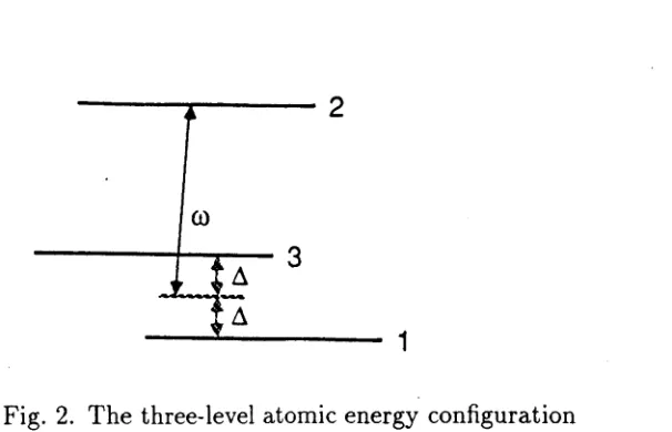
su-Fig. 2. The three-level atomic energy configuration

perposition of its ground states |1) and |3) (Fig.2) , using multi-atom injection to

the cavity and interacting with a single field mode, a large index of refraction with

vanishing absorption can be obtained [54]. This means that a large phase shift can

be obtained in their system. Can we improve the phase shift , and hence get a better

superposition state if we extend the two-level J-C system of the previous section to a

three-level system?

The dynamics of the atom and statistical properties of the field in this system

have been discussed in detail in the well known review of Yoo and Eberly [57]. where

the two-photon resonance condition is imposed and three different types of three-level

atom (A type, type and V type) are considered. Here, we only consider one of the

three types - A type three-level atom (Fig.2). The system is one A type three—level

atom interacting with a single quantized field mode. We first treat our system as

closed, i.e. no coupling of the atom with the radiation field modes of free space. The

13

rotating wave approximation is:

H = Ha + Hf + H (2.21)

where Ha and Hp are the free parts of the atom and the field respectively:

Ha = (2.22)

t = l

and

A A { A

Hp — ua' a (2.23)

we have taken h = 1 for simplicity and u;,(z — 1,2,3) is the ith atomic level transi­

tion frequency, uj is the mode frequency, 6/" and 6, are the creation and annihilation

operators of an electron at level i , while a1 and a are those of a photon in the mode.

{ M ,+ }=<$,,; (2.24)

[a, a^] = 1 (2.25)

we assume that direct dipole transitions are allowed between atomic levels 1 and 2 ,

and between 2 and 3, and forbidden between levels 1 and 3. After the RWA the dipole

interaction part, H ,is given by

H = gab^b\ + #<2^6362 -f h.c. (2.26)

same for each transition (see Fig. 2 ). Similar to the two-level J-C model, we separate

H into two parts Hi and ////, in which Hi consists of two obvious constant operators

of motion: total electron number operator Pe — bfb\ + b^b^ + 6 3 6 3 and excitation

number operator N = a^a -f 6^6 2. Both Hi and Hu are constants of the motion:

H = Hi + Hn (2.27)

and

[Hu Hn \ = 0 (2.28)

The eq.(2.28) implies that the time translation operator U(t) = exp(—iHt) factors to

Ui • Uh with

Ü , ( t )= e -" '* , U = e_iÄ" ‘ (2.29)

In the interaction picture, the Hamiltonian take the form:

H\ = loN + (u2 — ^)Pe (2.30)

Hu = - A b + k + Abfb3 + H' (2.31)

where the detuning parameters A are:

A = |cc?i21 — to = |^ 2 3 — (2.32)

15

exist three bare states :

|1><,1) = |l)|n>; |3)(n> = |3>|n); |2)<"> = |2>|n - 1) (2.33)

Using th e states |j ) n(j — l,2 ,3 ;n = 1,2...) as the basis, the m atrix representation of

H i and H u are:

Hi = (um + const.) • I

Hu

- A g \ f n 0

9 \ f i 0 9\[™

0 g\Jn A

where I is a 3 unit m atrix. The U[(t) is just a phase factor:

(2.34)

(2.35)

ü l ( t ) = e ~Hun+cox j _(2.36)

T he eigenvalues of Hu in eq.(2.35) are:

E, = A2 + 2 ff2n, E 2 = -A + 2S2" . 2 ^3 = 0 (2.37)

T he eigenstates are:

m V - A + ^ / A 2 + 2g'2n g^/n loUn) A + y/2g2n + A 2

w = 2 ^/a'2 + 2g2n 1 + +

i ^ r r l3> (2-38)

i ^ ) = ~ t : ^ + ,2 g - n ) w +

1^3) —

2V/A 2 + 2p2n

-Qy/n

|2)(") + i U A 2g2” -+ f 2 |3)(n) (2.39)

>/A2 + 2g2n|! ) (n)

-yj2g2n -f A 2

A

\j'2g2n -f A 2|2) (n) +

2y/2g2n + A 2

gs/n

From these equations, we obtain:

|2>‘-> = + - M ^ \ M +

A

\J A 2 + 2g2n. \ / A 2 + 2g2n >/A2 -f 2g2n1^3)

I D « “ ) =

2 V A 2 + 2<)2n 2V A 2 + 292n t/ A 2 + 2<?2n

(2.41)

l& ) (2.42)

iWn) A + y/A2 + 2g2n | M , A - y ^ A 2 + 2ff2n , j v , g y ^ , JV ^

^ 2v/A2 + 2 g2n + 2\/A 2 + 2#2n ^ + x/A2 + 292n ^ 3^ *

As th e first step, using the same m ethod as the ref.[52], a superposition of atom ic

states |1) and |3) can be obtained:

1 ^ ( 0 ) ) — ci 11) + C313) (2.44)

In the second step , a coherent state field interacting with the atom, the initial state

of the system is :

l'I'(O)) = |q) ® (ci11) + c313))

°° a n

= e x p ( - |o |2) + c313 )177)) n— 0 Vnl

OO f y T l

= e x p ( - H 2) ^ (Cl|P » ) + c 3|3 ) h „=0 v n !

|* « ) ) = t / |* ( 0 ))

(2.45)

(2.46)

17

If we take c\ = C3 = c in the initial state, then from eq(2.47),we get :

o 1 I^W> = c e x p ( - | o | 2) J 2 ~ / = {

n=o vn !

\ / A 2 + 2g2n — A

2 \ / A 2 + 2g2n exp( — + 2g2n t)

+ ^ v /n

\ / A 2 + 2g2n exp(—i ^ A 2 -f 2g2n t) — e x p ( i ^ A 2 + 2g2n t) |2)|ra — 1)

+

|3)|n)} (2.48)

In the dispersive limit, A > > 21 ,

yjA 2 + 2g2n « A +

A (2.49)

the time-evolved state Eq.(2.48) becomes:

W O ) = c e x p ( - | o | 2) ] T ^ = { e x p ( Z(A + I1)!71) + ^9 ^ exp(—z(A + ^ - ) 0

— exp(z( A + — )0 12)177 - 1) + exp z(A + ^ - ) t j |3)|n)} (2.50)

this is an entangled superposition of the atomic and field state. A radio-frequency

7t/2 pulse, identical to th at used in the preparation of the initial atomic superposition

transforms the state of Eq.(2.50) into the state:

wo>

+9 \ ß

(2.51)

A n a to m ic state m easurem ent on the state 11) or |3) th e n p ro je c ts th e fie ld in to the

state:

T h is is a su p e rp o s itio n o f tw o coherent states. W here the p lu s applies i f the a to m ic

state was m easured to be j l ) and the m inus applies if sta te |3) was m easured. T hus

s im ila rly to th e tw o level J-C m o d el scheme the su pe rp o s itio n state can be o b ta in e d

in a three level J-C m odel system in the large dispersive li m i t i f we do n ot consider

th e a to m ic lin e w id th .

C. T h e sem iclassical analysis o f the three-level J-C m o d el system

F rom the above, we can get th e su pe rp o sition state o f the fie ld in a th re e level system

b u t o n ly in the large dispersion lim it w ith a sm all phase s h ift. T h is is d iffe re n t fro m

th e m u lti-a to m in je c tio n scheme proposed by Scully. To get m ore in fo rm a tio n abo u t

one a to m case, we proceed sem iclassically, and consider th e A c o n fig u ra tio n (F ig .2).

T h e p o la riz a tio n P associated w ith the atom ic tra n s itio n s 3 —► 2 and 1 — > 2 is given

!*(<)) = c{e,AV ' £ ‘) ± e " AV - * ' ) } (2.52)

by [54, 55, 56]

19

where p23 and p2l are the transition matrix elements and p23 and p2\ the correspond­

ing density matrix elements. If, initially, the atom is in a coherent superposition state

of two ground-states, the initial density matrix for the atom is:

P =

p°22 0 0

0 P33 P 3 1

0 P ? 3 1

(2.54)

The atomic evolution equations are[54]:

I l

P23 = —{iw23 + 723)^23 — jTp23{p33 — P22)E — ~p2\p\3E (2.55)

l l

P21 = ~(^21 + 72l)/I * 321 — Tp2l(/hl — P22)E ~ ~p23P3\E (2.56)

h h

l

p31 = —( ^ ’31 + ')3l)p3\ ~ ~jr[P23p2l ~ p2\p32)E (2.57)

l

P\3 = —(^13 -f 713)^13 — j{p\2p23 ~~ P23P\2)E (2.58)

I

P22 = —12P22 — j [{P23P32 + P2l/>12)77 — C. C. ] (2.59)

I

P33 = ~l3P33 — J^(P*23P23 ~ C.C.)E (2.60)

I

P11 = - h P n ~ ji {Pnp2\ ~ c.c.)E (2.61)

where c.c. is the complex conjugate term, E is the field of the light with the frequency

v , 7i(i = 1,2,3) are the diagonal decay rates, 7 = 1,2, 3) are off-diagonal decay

rates and 7 = (7, + 7; )/2.

and p2i :

P 7 \ i£ o e -" " { P 2 .-— --

---n i A 2i + 721 - 7 2

i T f p - ^ * _ e - t A 2 i < - 7 2 l < l

P22 [e

P21T Pi 1 * A 2i + 721 - 7 i

1 P23/>31 “

zA 2 1 T 721 ~ 731 — ^ 3 1

e ~ 7 l < _ e i A 2 i < - 7 2 i < j

Jg —(‘>31+«*'3i)Z _ g-(721+IW21 )Zj I _(2.62)

P 23 • ■ “" { P 2 3 - T ---A I « ' 72' - e - A23‘ - ™ ‘ ] Z A 23 + 7 2 3 — 7 2

P33

‘23 + 7 2 3 — 7 3

1

-73* _ g*A23Z-723n

(2.63)

where E = Eoe~lut, E0 is the electric field amplitude of the light. If all of the

damping terms in these equations are put equal to zero, 7, = 0, then the equations

are equivalent to a Hamiltonian system, with J —C coupling between the levels. So

we can compare with the result of the previous section.

From Eqs(2.53),(2.62), and (2.63), we get Fig.(3). It shows us that, if one three-

level atom interacts with a single mode field, only at some special times is the dis­

persion of the atom nonzero while the absorption of the atom is zero ( Points A and

B in Fig.3 ). It is impossible to get a atomic state which has stable zero absorption

and nonzero dispersion over a long time in the case of single atom interacting with

21

J 0.0

20.0 40.0 60.0

INTERACTION TIME gt

Fig. 3. Dispersive (R e P) and absorptive (I m P) parts of polarization vs the scaled in­ teraction time gt in the system of one three-level atom interacting with one field mode. The values of parameters are u>3i = 0.05, A 2i = 0 . 1 , p33 = pQu = 0.5,

= 72 = 73 = 0. Dashed line: absorption , Solid line: dispersion

dispersion and zero absorption were obtained because of the accumulational effect of

m ulti-atom interacting with the optical field. Because the phase shift is in proportion

to the dispersion and the interaction time, the semiclassical result we obtained here

means th a t the optical field cannot get a large phase shift after one three-level atom

interacting with the optical field. Hence the refractive index enhancement scheme of

Scully and Zhu [54] does not appear to be applicable to the superposition generating

CHAPTER III

A TO M IC L IN E W ID T H P R E V E N T S

M A C R O SC O P IC S U P E R P O S IT IO N

G E N E R A T IO N

In chapter II, a scheme for generation of macroscopic quantum superposition states

using a three-level J-C model system was suggested. The result is similar to the

two-level J-C model system. In these schemes, the effect of atomic linewidth was not

considered and the coupling coefficient g was assumed to be time independent. In

this chapter, we show that the scheme does not work when the atomic linewidth is

included[14].

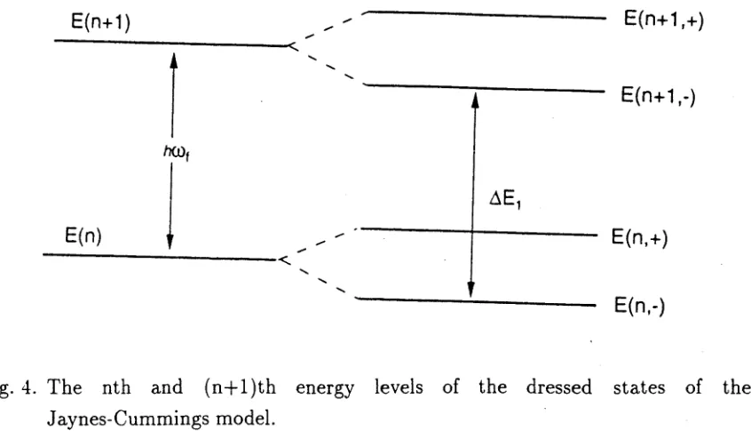
From Eq.(2.7), we know that the eigenvalues of these dressed states are

£ ( n ,± ) = (n - ^)hu>j ± + ng2)? (3.1)

This means that in the dressed state basis the equal-spaced energy ladder of the

harmonic oscillator is split into two “ladders”. The “plus" and “minus" ladders

E(n+1) E(n+1,+)

AtCO,

E(n)

E(n+1,-)

E(n,+)

E(n,-)

F ig . 4. T he n th and ( n - f l ) t h energy levels o f the dressed states o f the

Jaynes-C um m ings m odel.

N e ith e r ladder is e q u a lly spaced. As described in re f [52], the a to m is in it ia lly prepared

in a state | 4 (0)),

W ( 0 ) ) = l ~ ) , ~ l + )!’ (3.2)

and the fie ld is in the coherent state \ a ) . Because | + )5 (refer F ig .2) is not in te ra c tin g

w ith the field, we are interested in the e v o lu tio n o f the coherent sta te o n ly when

in te ra c tin g w ith the levels | — ) g and | T) e. T he in itia l a to m -fie ld s ta te is the n

W O » = e x p (—^ - ) A = j | n ) | - ) 3 n = 0 v n .

In terms of the dressed states , this becomes

From Equation (2.5), In the dispersive limit A —* oo this approaches

(3.5)

So only the lower ladder dressed states are present. From Eq(3.1), the spacing of

adjacent minus ladder states is

Since this is a function of n, they are not equally spaced. However, for a large-

amplitude coherent state field , the energy spacing is approximately constant:

From the harmonic oscillator we know that if the energy spectrum of a system is an

infinite equally-spaced ladder, then there exist coherent states for that system whose

complex amplitudes evolves like aexp(zu^), where Tiw is the spacing between adjacent

energy levels. Moreover if the energy spectrum of a system is given by two ladders

of different spacing there will exist states which are effectively superpositions of two AJSi(n) = huj j - + (n + l)s 2)j - ( ^ - + n$2)!] (3.6)

AEl

«

I»,,

-

A + w v ) - i

1 4 (3.7)

25

the spacing of that ladder. This is the sort of dynamics proposed in ref. [52] to gen­

erate macroscopic superpositions of coherent states. The coherent states associated

with the different ladders will rotate at different frequencies and can eventually be­

come macroscopically separated in phase. So the equal spacing of the energy levels,

Eq.(3.7), makes the initial state Eq.(3.5) evolve as a coherent state of the lower ladder,

rotating at the frequency :

(3.8)

It has a frequency lower than that of the free field by the detuning:

In the dispersive limit |A| 2|a|g, Eq.(3.8) becomes:

<i> = u f - g 2/ A (3.9)

As was found by a different method in Chapter II, a superposition of two coherent

states is obtained:

I«'(<)) = I a e - “' 1) + |ae- "*<) (3.10)

with t the field-atom interaction time. This is equivalent to the result of equation(2.20).

Now, we assume the atomic transition has a linewidth, 7. The standard J-C

E(n+1)

0

,

E(n) v

. . . • •

SS> ' .k' ^ v • ? * § h 5 f c v * ‘

^ m a x ( E | + 1 .*)

Fig. 5. The dressed state energy levels are “spread" when the atomic linewidth is considered.

when the linewidth is included. However the the effect of the linewidth can be u n d e r­

stood from physical considerations. The linewidth will produce a similar linewidth of

the dressed state energy levels (Fig.5). The mechanism giving rise to the superposi­

tions relies on the spacings of the dressed state ladder being different to the spacing

of the free oscillator ladder. For the free field and interacting coherent states to be­

come separated, it is necessary that the linewidth induced range of detunings does

not extend to zero. For then there would be an overlap with the free coherent state,

27

Fig.5, the maximum of the broadened energy level E(n -f 1, —) is approximately

Emax{n + 1 ,- ) = (n + ^)hujf - + (n + 1)^2)]= (3.11)

and the minimum of the broadened energy level E ( n, —) is

Emin(n, - ) = (n - ^)hcoj - ^ [ 1 ^ - i- lL + ng2)]* (3.12)

An estimate of the largest frequency difference between the dressed states is then

A E2 = hujf — ft([— —— h {n + 1)</2]2 — [~ ~ f n92]2) (3.13)

4 4

Hence for the interacting state to become well separated from the free field coherent

state will require that the following strong inequality be fulfilled:

[{S- +; ' ~2- + ng2]i « [(A ~ 7)2 + (n + l ) g ^ (3.14)

4 4

This requires, g2 >> 7A. Assuming A > 7, then

92 » 72. (3.15)

At the same time we require the two coherent states \ae~lu,ft) and |ae~lcpt) in Eq.(3.10)

to be separated. Hence the scalar product of these coherent states should satisfy:

\{aelu>t\ae~l<t>t)|2 = exp( — \a — ae*52^ A|2) < - . (3.16) e

a to m and th e fie ld is T ( 0 < t < T ), th is requires

g T > 1 (3.17)

So to get a m a cro sco p ica lly d is tin g u is h a b le q u a n tu m su p e rp o s itio n state, the c o n d i­

tio n s (3.15) and (3.17) m ust b o th be satisfied. H ow ever, th e co u p lin g coefficient g

and lin e w id th ,7, are re la ted . T he co u p lin g c o efficie n t is given by [59]:

9 2 = ( ^ T " ) l w|2’ (3-18)

w here u is th e n orm a liz e d mode fu n c tio n . W e assume th a t th e fie ld is a single-m ode

pla ne wave. Its le n g th c T is d e te rm ine d by th e to ta l in te ra c tio n tim e and its m in im u m

cross section by th e lig h t ’s w avelength / . T h e n th e m ode fu n c tio n is :

u = (c T A2) - h (3.19)

So fro m E q.(3.1S ) we fin d th a t the m a g n itu d e o f th e c o u p lin g coefficient g is d e te r­

m in e d by the to ta l in te ra c tio n tim e T ,

2 _ _§7_

9 8jtT

S u b s titu tin g E q.(3 .2 0) in to E q.(3.15) and (3.17), we o b ta in ,

7T < < 3_

$7T

(3.20)

29

7T > (3.22)

These are contradictory conditions that cannot be simultaneously satisfied by the

system. Thus the linewidth of the atomic transitions will always wash out any sepa­

ration of coherent states for free-space modes. The underlying reason that the atomic

linewidth prevents the formation of well separated superposed coherent states is the

inverse dependence of the atom-field coupling strength on the interaction time. This

is because we have used free space modes whose mode volume increases with the

interaction time. To prevent smearing out of the coherent state frequencies the cou­

pling strength must exceed the linewidth, as in inequality (3.15). This requires a

sufficiently short interaction time. This is incompatible with the interaction time

being sufficiently long to separate the interacting and non-interacting coherent states

by more than the phase uncertainty of the coherent state.

In conclusion, we note that a scheme for preparing a macroscopic quantum su­

perposition state has recently been proposed by Brune et al. [22]. This scheme is

related to that of ref.[52], however it uses a high Q microwave cavity to overcome the

linewidth problem discussed in this paper. It is remarkable that sufficiently high Qs

CHAPTER IV

T H E CLASSICAL C H AO TIC B E H A V IO R OF

SE C O N D H A R M O N IC G E N E R A T IO N

A. Chaos

Since the first international conference on chaos in classical dynamical systems took

place in 1977, chaos has been studied extensively. Great progress has been made in

understanding the qualitative behavior of classical dynamical systems, and chaotic

phenomena have been found in many classical systems [4]. Chaotic behavior is in­

herent in most nonlinear mechanical systems since many orbits have a “sensitive de­

pendence on their initial conditions’*. Physically, this means that (arbitrarily) small

changes in the initial conditions can rapidly cause very large changes in the ensuing or­

bit. This implies that no matter how much past behavior we experimentally observe,

we can not predict much of the future behavior of such orbits, due to the inherent

experimental error in that observation. Mathematically, chaos is a phenomenon that

31

and can be easily (although numerically) found in some equations. We now review

the mathematics of chaos, following ref. [60]. Let us consider a system described by

first-order differential equations:

Where i = 1,2 -•• , N and x(t) is the N-dimensional vector with components x,-. F,

are nonlinear functions. For any initial state x(0) of the system, we can solve the

equations to obtained the future state x(t) of the system for t > 0. And because these

equations are first order in the time derivative, they describe unique trajectories given

the initial conditions. Chaos is defined as a sensitive dependence of the trajectory x(t)

on the initial conditions. This sensitive dependence can be quantitatively described

by introducing the concept of a Lyapunov exponent [61]. It is a measure of the rate of

divergence ( or convergence ) of initially infinitesimally separated trajectories. First

consider the instantaneous, local linearization around the trajectory x(t) at time t.

For a short time, Ax evolves according to

J X ;(<) = F,(x(t)) (4.1)

— Ax, = Jj,tA (4.2)

where Jo, is the Jacobi matrix defined by

As the trajectory evolves in time, the matrix elements J also evolve. At each

instant of time, the eigenvalues of J can be calculated. If at least one eigenvalue has

a positive real part, the local magnitude of Ax grows. Such a tendency is averaged

over the course of the trajectory and this leads to the definition of the Lyapunov

exponent[61]:

A = lim A l n ^ j

t-+oo,d(Xo,0)—>0 \yt a(xo, 0 ) /

d(x0) = ||Ax(x(0), t)\\ (4.5)

where d(x0) is the length of the deviation vector at time t that started at t = 0 from

x = X o - The notation || || means the Euclidean metric in an N-dimensional space.

Any trajectory of a dissipative system will approach a bounded region of phase

space called an attractor, as t —> oo. Attractors include points, limit cycles, and

chaotic cycles. If A > 0, the nonlinear system exhibits chaos, initial trajectories

moving apart with an initial exponential rate A. This is referred to as sensitive

dependence on initial conditions. For dissipative systems, a stretching in one direction

has to be accompanied by a more-than-compensating contraction in other directions.

The phase space trajectories for a chaotic system asymptotically approach a strange

attractor, an attractor with a fractional dimension. If A < 0, the trajectories approach

33

T

_{¥ //////,}

V/////A

Nonlinear

crystal

T

l

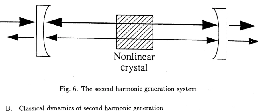
Fig. 6. The second harmonic generation system

B. Classical dynamics of second harmonic generation

Second harmonic generation is a well-studied problem in both classical and quantum

theory [64, 70, 75]. In this system, the nonlinear crystal is placed inside a dissipative

driven optical cavity, and light at the fundamental frequency u j interacts with the

crystal and is frequency doubled to its second harmonic 2uj (Fig.6). The system is

dissipative because light is lost through the cavity's partially transmitting mirrors.

This loss is modeled by the coupling through the mirrors of the cavity modes to

the reservoirs of field modes outside the cavity. The classical dynamical equations

can obtained by applying Maxwell's classical theory to second harmonic generation.

These equations are [75]:

oil — — i Aioi — kioti \ Qio 2 T E (4.6)

where a i and a 2 are the complex amplitudes of the fundamental mode and the sec­

ond harmonic mode respectively, and E is the pumping field. These equations are

nonlinear, have four real variables (since cq and a 2 are complex), and are known to

have a range of attractors: fixed points, limit cycles and chaotic [64, 75]. Hence this

system is an interesting one in which to investigate how classical attractors arise from

the underlying quantum mechanical description of second harmonic generation. To

simplify, let us introduce dimensionless scaling, denoted by tildes. The above classical

equations become:

= E -f (“ iAi - l) Qi + a \a 2 (4.8)

^ = (-t'Ä 2 - fc) q2 - (4.9)

Here d, = ( x /^ i)<*,-, E = E ( x / kJ), k = k2/k\, A, = A t//q , r = tk\. These scaled

equations depend only on the scaled parameters E, A, , and k . So varying the ratio

x/k\

fixed. We call the ratio x/^'i the scaling parameter and denote it by S:

s = x / h

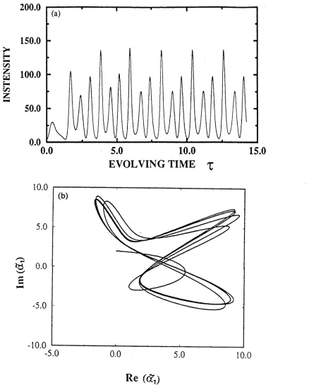
The mean photon numbers and phase space orbits in the classical chaotic region,

limit cycle and fixed point are shown in Fig.7, Fig.8 and Fig.9 that we got by solving

35

systems from classical dynamical theory. In Chapter VI, we will investigate the cor­

responding behaviors using the quantum trajectory method and study the transition

from quantum chaos to classical chaos. The driving field amplitude is E = E K \ / S , so

the classical limit of strong driving is obtained by decreasing the scaling parameter S

with fixed E, A, and K . Taking the limit S —► 0 does not change the scaled classical

equations (4.8),(4.9). Hence scaling allows quantum solutions for arbitrary S to be

5.0

10.0

EVOLVING TIME

ReCd,)

Fig. 7. The classical chaotic cycle of the fundamental mode, (a) The scaled mean photon number |d ] | 2 as a function of time, (b) The scaled field amplitude

INS

TE

NSI

TY

37

100.0

-5.0 10.0

EVOLVING TIM E x

Re (<?7)

Im

(a

,)

IN

TEN

SI

TY

EVOLVING TIME

x

Re (a,)

39

CHAPTER V

Q U A N T U M CHAOS A N D Q U A N T U M

T R A JE C T O R Y M E TH O D

Quantum mechanics has been very successful. However, the quantum mechanical

origin of chaos in classical physical systems remains to be fully understood. A con­

spicuous puzzle has been how to reconcile this nonlinear, classical phenomenon with

the underlying linear quantum theory. If we believe that all of physics is funda­

mentally quantum mechanical in nature, the classical chaos must emerge from the

quantum theory.

In classical statistical physics there are two ways of approaching the dynamical

evolution of a system. In the first the system is described by a probability distribution,

and a Fokker—Planck equation, or its equivalent, generates the evolution in time. In

the second the system is described by an ensemble of noisy trajectories, and a set of

stochastic differential equations are used to generate the trajectories.

The standard quantum mechanical method is solving the master equation of

version of a probability distribution. Because the master equation is difficult to solve

analytically, it is often solved numerically. If the relevant Hilbert space of the quantum

system has a dimension N, the number of the elements of the density matrices we

need to calculate is N 2. If the system consists of two modes, the number of density

matrix elements, will increase to (Ah x N2)2. If N >> 1 then the later numbers are

too large to realistically calculate. Thus many problems cannot be investigated well.

To settle this problem, a quantum mechanical version of the classical stochastic

trajectories has been developed in the past couple of years. It is known as the quantum

trajectory method or the Monte Carlo wave-function method[33, 34, 35, 36]. This new

method for solving the master equation is based on a stochastic Schrödinger equation

and has been interpreted as providing realizations of individual quantum trajectories

[33, 73]. It is mathematically equivalent to the quantum state diffusion approach

of Gisin and Percival[37]. The method consists of two elements: evolution with a

nonhermitian Hamiltonian and randomly decided quantum jumps. It solves a wave-

function equation instead of a density operator equation; the number of variables

involved in a wave function treatment (~ N) being much smaller than the number

required for calculations with density matrices (~ N 2). In this method, each of the

trajectories describes one possible path that the system may take through the Hilbert

41

When a quantum field tends to the classical limit, the effect of quantum jumping

is much smaller than the strength of the field so that the configuration of the time

evolution behavior of every single trajectory of the ensemble is like the classical tra­

jectory. However, every trajectory is different from other trajectories due to the effect

of quantum jumping. An ensemble average or time average is equivalent to the result

of a standard master equation calculation in quantum theory [33, 34, 35, 72, 74].

Classical chaos encompasses two major types of behavior: Hamiltonian chaos in

which energy is conserved, and dissipative chaos. Much work has been concerned

with conservative systems in which the semiclassical method has proved particularly

fruitful [31, 63]. However classical physical systems are often dissipative and so dissi­

pative quantum systems have also been studied [67, 68, 69]. For example it has been

shown for a laser with a classical Lorenz attractor, that the quantum mechanical

Wigner distribution reduces to the classical invariant measure on the attractor in the

classical limit of large photon number [42].

Previous work on second harmonic generation has analyzed the dynamics of

the Q-function, a quantum mechanical quasi-probability distribution, for the case of

classical limit cycles [25]. In the classically chaotic regime the steady state solutions of

the master equation have been numerically determined and compared to the classical

towards the classical limit was quite limited due to the computational demands of

the problem. Nevertheless some correspondence between the classical and quantum

mechanical solutions has been reported [70].

A. Quantum trajectories method.

In the method of quantum trajectories, the dynamical object is a wave function

rather than a density operator. The wavefunction is generated stochastically and it is

ensembles of these wavefunction that are equivalent to the master equation solution.

It can be shown that averages of operator mean values over wavefunction ensembles

reproduce the mean values generated by the master equation [33]. In order to make

the thesis reasonably self-contained, we briefly introduce the method of quantum

trajectories closely following the reference [33].

The quantum trajectory approach is built around the theory of photoelectric

detection and the master equation of photoemission source. Using the two theories one

can relate the statistics of photoelectron emissions to a dynamical process involving

photon emissions taking place at the source. Now let us consider the general source

master equation of dissipative systems. It describes the quantum mechanical evolution

of a system interacting with a reservoir and the master equation is:

43

The formal solution of the master equation is:

p(t ) = 0) (5.2)

The physical process of the source described by equations (5.1) and (5.2) includes both

evolving and photoemission of the source. The operator L also includes two parts —

evolving operator and photoemission operator. If the photoemission is described by

a superoperator i?, adding and subtracting the superoperator R to T, the equation

(5.2) becomes :

p(t) = e[(l-B)+«]‘p(o) (5.3)

By means of the equation:

p[(L + h. R)x\ = T a k r d x k R dxk-i---r R e U '

(5.4)

the equation (5.3) can be expanded in terms of the superoperators ( L — R) and R:

~ f t R m

p{t) — 'y ) / d t m / d tm—] n ^ O J o J o

t • • ■ k e (L- k ) hp(0)

Jo

(5.5)

Now the quantity inside the integrals is the unnormalized conditioned density operator

p c{t) for an initial state pc(0) = p(0), where the over-bar denotes unnormalized.

Eq.(5.5) can be interpreted as a generalized sum over all the photon emission pathways

may involve any number of photon emissions, from m = 0 to m — oo, and the times

of the emissions can be any ordered sequence of m times in the interval [0,t]. The

quantum trajectory method is a simulation of the physical process. The basic method

is to define a conditioned density operator pc(t) , let it be equivalent to the inside the

integrals on the right-hand side of Eq.(5.5), take it out and normalize it, then give

it a physical interpretation in term of evolution without photon emission interrupted

by collapses at the time of the photon emission. At time t, for an initial state /5(0)

and a particular sequence of photon emission times, the conditioned source density

operator is given by

JcW

T

with

J c(t) = o) (5.7)

This procedure decomposes the quantum master equation into an infinity of quantum

paths, or quantum trajectories. The trajectories include two processes — evolution

without photon emission governed by the superoperator (L — R), and collapses with

the emission of a photon as described by R.

The conditioned density operator pc{t) usually can be factorized as a pure state:

45

we also write

U t ) = |T«(0X*«(0l (5.9)

then the propagator for the density operator pc(t) is replaced by a propagator

for the state |'PC(£)). Propagation without photon emission over a time At is given

by

I^c(< + AO) = e-Wfi>"A‘|$ c(<)) (5.10)

where H is a nonhermitean Hamiltonian. When a photon emission occur, the unnor­

malized state undergoes a collapse:

l*c(0) - <?|T«(0> (5 .ii)

where C is the annihilation operator of the source field and its relationship with the

superoperator R is Rp = CpC^.

When a weak light is observed by a photodetector, a series of individual photo-

electron is emitted at random point of time. We cannot predict that a photoelectron

will definitely be emitted at this particular time or that particular time. So the emis­

sion times of the photons of the source are random too. If the conditioned density

operator at time t is pc(<), the probability that an emission occurs in the interval

[ t , t-f At] is [33] :

('M f)|C 't C|'I'c(0}A< (5.12)

where pc(t) is the conditioned density operator at time £, and |T C(£)) is the wavefunc-

tion corresponding to the conditioned density operator. The numerical simulation

uses discrete time, with a time step At and follows a three step wavefunction evolu­

tion algorithm: (i) Evolution for a small time A t of the wave function governed by

Eq.(5.10). (ii) Calculate the collapse probability of the wavefunction and generate

a random number rn distributed uniformly on the interval [0,1]. (iii) Compare the

collapse probability with r n and calculate the wavefunction according to the rule:

B. Master equation of second harmonic generation

Investigation of the second harmonic generation system is quite well established by

many authors in both the quantum and the classical region. A well known approxi­

mation scheme results in a quantum optical master equation [23, 24]. Denoting the

fundamental cavity mode quantities by a subscript 1 and the second harmonic cavity

I'MWi)} = (5.13)

(5.14)

47

second harmonic generation is [25, 26]

-Jj = —[HD + HI + HE, p ] - \ - k i ( 2 ä i p ä \ - ä \ ä i ß - p ä \ ä i

+ k 2 (^2a2p a \ — a \ a 2p - p a \ a ^ j (5.15)

He = h A i ä \ ä i -f h A 2a \ a 2 (5.16)

H i = i ^ X ( a + 2a2 - ä j ä | ) (5.17)

He — ihE faj — j (5.18)

where h\ and a2are the boson operators for the fundamental mode and the second

harmonic mode respectively, and \ is the nonlinear interaction strength. E is the

driving field strength and is proportional to the amplitude of the coherent state

assumed to be driving the fundamental cavity mode [27]. Without any nonlinear

interaction, \ = 0 , mode 1 is driven into a coherent state of amplitude E /k . p is the

reduced density operator of the cavity modes obtained by tracing over the reservoirs.

Ai = lji — itje , A2 = lo2 — 2u>£, where Ai and A2 are the detuning of the cavity modes

from the driving field ( with frequency uje ) and its second harmonic respectively. k\

C. Quantum trajectories in second harmonic generation

The quantum trajectory theory is built around the theory of photoelectric detection

and the master equation theory of photoemissive sources. According to the master

equation (5.15) and following the general quantum trajectory theory presented in

Section A [33], we deal with the second harmonic system by the quantum trajectory

method. Taking R\ = 2Aqdi/5dJ, R2 = 2k2a2pa'2 to be the collapse superoperators for

the Lüi and cc2 modes respectively, the superoperators L — R\ — R 2, R\ and R 2 that

govern the evolution and collapse, respectively, are defined by:

CMc)(4'c

icj ,

= C 2 \ l p c ) { ' p c

\c\

(5.21)

where pc is the unnormalized conditioned density operator. |

ipc

49

harmonic mode, and

Pe=He)Hc\

C\

\j2k\ ä\

C2

2k2

The conditioned density operator may be written in terms of a pure state wavefunc-

tion:

Pc(t)

=

I

and

[He He

Between photon emissions, the unnormalized wavefunction H e ) is governed by the

nonunitary Schrödinger Eq:

j t

\JC) = ^H\A)

with the nonhermitean Hamiltonian:

H = Hd+ Hi + He

—

the unnormalized wavefunction H c H ) ) can written as:

Hc(t) ) = Cn,mW,m) n , m

Substitute Eq.(5.28) and Eq.(5.29) into Eq.(5.27) to find:

n , m

^ ^ C 'n ,m TTl) — h(Aidffii + A 2ä\ä2) + y x ( a l2ö2 - o.\a\)

+ ihE(ä\ — ä j ) — ihk\ä\ä\ — ihk2ä\a2 ^ C„iTn|n, m) J n , m

= ~ ki)n+ { -iA 2 - k2)m\Cn,m\n,m) n ,m

+ ^ Z l ( \ / ( n + 1)Cn+i,m\n,m) - y /nCn-i,m\n,m)) n ,m

+ H o W (n ~ 1)n (m + l ) C n- 2,m+\\n,m) n ,m

- y j { n + 2)(n + l ) m C n+2,m- i |n, m>) (5.30)

So we get:

(-'n ,m — E T 1 ^ n + l , m V ^ " ^ n — l , m j T [( 2 ^ 1 ^ 1 4 ( ? - ^ 2 ^2) ^ ^ ] ^ n , m

(5.31) \/(rc ~ 1 )n(m + 1) Cn_2,m+i ~ \J(n + 2)(n + l)m Cn + 2 , m — 1

The evolution is interrupted by instantaneous collapse at the times of the photon

emission:

I<M0) — * Ci\ipc{t)) , (5.32)

I*Pc{t)) — > C2\^c(t)) > (5.33)

51

(5.34)

n, m

C ^ c M ) = >/5feÄ2|0e(t))

= > / % E C » . m +i v O T | n , m ) . (5.35)

n, m

The probability of a collapse occurring in the interval [£, 2 T At] is given by:

f t( l) Tr[Ripc(t)]At

(^c(f)|abl|V ’e(0) (^c(t)l^c(<))

a ( 2 ) 7>[fi2pc(<)]At

9( (V’ctOlabzI’/’ct*)) - 2 ^ .(0 l^ c(0 >

(5.36)

(5.37)

( ^ ( * ) I W i ) > = E I C - . m l2 V (5.38) n, m

(^ c( t) |a |a i|^ c(<)) = n|Cn,m|2 , (5.39)

n, m

( ^ c ( < ) | a j a2| ^ c (0> = 5I m l^ . ^ | 2 • (5.40) n, m

The equations (5.27) — (5.40) define a single quantum trajectory of the second har­

monic generation system. An ensemble average over infinite quantum trajectories,

taken with respect to this conditioned wave function, reproduces the results of a

D. Q-function in second harmonic system

The Q function, also known as the Husimi distribution, is a function of coherent state

complex amplitudes of the fundamental mode au and the second harmonic mode a 2 :

Q(<xi , a 2) = ( ( a 2| 0 (q i|)/3(|q i) ® | a 2)) (h.41)

It may be interpreted as the probability distribution for the fields to have the complex

amplitudes and a 2 [5, 77]. In the classical limit oq and a 2 can be interpreted as the

classical complex field amplitudes [76], and the Q function is expected to approach the

classical phase space probability distribution. To present the steady-states graphically

each mode is considered separately. Tracing over one mode generates a reduced

density operator for the other mode:

P\ — T r 2(p), p2 = Tr l (p) (5.42)

The Q function for each mode is:

Qi = (ai\pi\ai), i = 1,2 (5.43)

The equations (5.27) — (5.40) define a single quantum trajectory of the second

53

I'J'i) = J 2 C ( n , m ) \ n , m ) n ,m

(5.44)

( ^ i| = C * ( n , m ) ( n , m \ (5.45)

n,ra

T he density operator for each trajecto ry can be obtained by.

p i = | 4 ' i ) { ^ . l

= ^ 2 C (n , m ) C ' ( n \ m')\n, m ) ( n \ m'\ (5.46) n,m n \ m '

The elem ent of the system density m atrix is

p n ,n ',m ,m ' = C(n, m)C*(n'm') (5.47)

Here n and m stand for mode one and mode two respectively. Using eqs. (5.4‘2)and

(5.46), we can find the reduced density operators for mode one and m ode two,

P i = C ( n , m ) C m(n '1m)\n)(n'\

n,n' ,m

(5.48)

p2 = C ( n , m ) C * ( n , m ' ) \ m ) ( m ' \ (5.49)

the elem ent of the m atrix is:

p i ( n , n ' ) = y C ( n , m)C*(n', m) m

(5.50)

p2(mi m') = Y l ^ ( n 5 m)C*(n, m') (5.51)