Probabilistic decision making with spikes: From ISI distributions to behaviour via information gain

White Rose Research Online

Universities of Leeds, Sheffield and York

http://eprints.whiterose.ac.uk/

This is a copy of the final published version of a paper published via gold open access

in

PLoS One

.

This open access article is distributed under the terms of the Creative Commons

Attribution Licence (http://creativecommons.org/licenses/by/4.0/) which permits

unrestricted use, distribution, and reproduction in any medium, provided the

original work is properly cited.

White Rose Research Online URL for this paper:

http://eprints.whiterose.ac.uk/86438

Published paper

Probabilistic Decision Making with Spikes:

From ISI Distributions to Behaviour via

Information Gain

Javier A. Caballero1,2_{, Nathan F. Lepora}3,4_{, Kevin N. Gurney}1_*

1Dept of Psychology, University of Sheffield, Sheffield, UK,2Faculty of Life Sciences, University of Manchester, Manchester, UK,3Dept of Engineering Mathematics, University of Bristol, Bristol, UK,4Bristol Robotics Laboratory, University of Bristol and University of the West of England, Bristol, UK

*[email protected]

Abstract

Computational theories of decision making in the brain usually assume that sensory 'evi-dence' is accumulated supporting a number of hypotheses, and that the first accumulator to reach threshold triggers a decision in favour of its associated hypothesis. However, the evi-dence is often assumed to occur as a continuous process whose origins are somewhat ab-stract, with no direct link to the neural signals - action potentials or 'spikes' - that must ultimately form the substrate for decision making in the brain. Here we introduce a new vari-ant of the well-known multi-hypothesis sequential probability ratio test (MSPRT) for decision making whose evidence observations consist of the basic unit of neural signalling - the inter-spike interval (ISI) - and which is based on a new form of the likelihood function. We dub this mechanism s-MSPRT and show its precise form for a range of realistic ISI distribu-tions with positive support. In this way we show that, at the level of spikes, the refractory pe-riod may actually facilitate shorter decision times, and that the mechanism is robust against poor choice of the hypothesized data distribution. We show that s-MSPRT performance is related to the Kullback-Leibler divergence (KLD) or information gain between ISI distribu-tions, through which we are able to link neural signalling to psychophysical observation at the behavioural level. Thus, we find the mean information needed for a decision is constant, thereby offering an account of Hick's law (relating decision time to the number of choices). Further, the mean decision time of s-MSPRT shows a power law dependence on the KLD offering an account of Piéron's law (relating reaction time to stimulus intensity). These re-sults show the foundations for a research programme in which spike train analysis can be made the basis for predictions about behavior in multi-alternative choice tasks.

Introduction

The decisions we make every day rely on processing continually refreshed streams of uncertain information. This information guides our choices, until some assumed termination criterion is

OPEN ACCESS

Citation:Caballero JA, Lepora NF, Gurney KN (2015) Probabilistic Decision Making with Spikes: From ISI Distributions to Behaviour via Information Gain. PLoS ONE 10(4): e0124787. doi:10.1371/ journal.pone.0124787

Academic Editor:Maurice J. Chacron, McGill University, CANADA

Received:October 9, 2014

Accepted:March 5, 2015

Published:April 29, 2015

Copyright:© 2015 Caballero et al. This is an open access article distributed under the terms of the Creative Commons Attribution License, which permits unrestricted use, distribution, and reproduction in any medium, provided the original author and source are credited.

Data Availability Statement:All relevant data are available within the paper and fromhttp://www. neuralsignal.org/index_data.htmlwithin the Macaque database via accession number nsa2004.1.

reached, upon which a decision is made [1–6]. Previous influential frameworks have addressed the concerns of uncertainty and time continuity by assuming that new information orevidence

occurs as continuous stochastic processes [1,7–10], often mapped at the level of the membrane potential of individual neurons [11–14]. However, most of the ensuing mechanisms are not naturally suited to exploit the statistical structure of the discrete and irregular sequences of ac-tion potentials that must ultimately form the substrate for decision making in the brain. As no-table exceptions, [15–17] assumed that evidence is sampled from Poisson processes and that statistical inference is conducted upon them. However, their result is founded on the assump-tionthat, for Poisson-based spike trains, the evidence was given by counting spikes, and it is not apparent what theoretical foundation might underly this assumption.

Further, there is, as yet, no clear way of dealing with spike trains with arbitrary inter-spike-interval (ISI) statistics, although there has been some interest in log-ISIs as means for sampling for decision formation [18]. Almost all previous models of decision making have worked at a more abstract behavioural level, where the interpretation of evidence is less constrained. Hence, they have either assumed the evidence is Gaussian distributed (e.g.[1,7,8,10]) or they have used a general formalism with no distribution specified (e.g.[19]). Both views have issues: the negative tail of the Gaussian makes it conceptually inadequate for describing ISIs (or their inverse, the instantaneous firing rate) and better fits are to be had with other skewed probabili-ty densiprobabili-ty functions (pdfs); while the general view does not provide any connection with neural mechanisms, in particular spikes. Typical neural recordings show spike trains which cannot be described by Poisson processes (e.g.see [11,20–27]) and these should be amenable to the same theoretical analysis as their Poisson counterparts. Fortunately, there has been considerable at-tention paid to identifying the particular pdf that adequately describes variables like these [20,

22,23,26,27]: it is known that the typical distribution of ISIs is positively skewed and has a non-zero mode (maximum). Any neurally grounded account of decision making must accom-modate these data.

To address these issues, we introduce here, a general approach to decision making with spikes based only on the assumption that evidence for decisions is conveyed in the distribution of ISIs. Thus, our premise is that the arrival of spikes provides the primary basis of information transfer and that the ISI provides the basic‘unit of evidence’. The ISI is therefore considered to be an‘atomic’time interval that is not linked to some more fundamental, continuous-time pro-cess (as is often the case). Our proposal gravitates around a novel variant of the likelihood func-tion which can be applied to any Bayesian or frequentist inference algorithm that uses

sequential sampling (for excellent reviews see [9,28]). With this likelihood we produce a new principled and general formulation of a statistical inference procedure known as the multi-hy-pothesis sequential probability ratio test [29] (MSPRT). We dub this mechanismspiking

MSPRTor simply s-MSPRT.

This novel and more general spike-based account allows us to address several previously un-answered questions. This was made possible by investigating several particular cases of the s-MSPRT, each of which assumed a pdf compatible with the distribution of ISIs in existing data [30,31]. First, noting that the non-zero mode in typical ISI distributions is dictated by an inter-spike refractory period, we ask, what is the advantage of such shape? The refractory period is often seen as drawback for information transmission, but we show it actually furnishes ISIs with additional information for discrimination, thereby facilitating their ability to inform decision making.

Second, given the diversity of s-MSPRT instances now possible, how robust is decision mak-ing if the distributions tested-for (the basis of the particular s-MSPRT) are not the same as

those of the data being tested? Hitherto, this issue has not been as acute because of the assump-tion of Gaussian signals and test-distribuassump-tions. However, as well as parametric differences be-tween test and data distributions, we now have to consider the possibility of a fundamental mismatch between the two, reflecting a potential‘ignorance’of the algorithms regarding the ac-tual statistical structure of the task [32]. Here, we show that this issue does not fundamentally compromise the s-MSPRT, thereby revealing a robustness we might expect of a

biological mechanism.

Finally we ask, what are the implications of positing aneural-levelmechanism for decision making like s-MSPRT, at the behavioural level? Our starting point for this analysis is the obser-vation that the mean decision sample size (meandecision samplefor short) of our algorithms is intimately related to the discrimination information between the distributions of the input data streams, as measured by the Kullback-Leibler divergence (KLD) [33,34]. Based on this, we demonstrate that the mean total information needed to reach any particular decision is con-stant and thus conserved. We show how this postulate gives rise to an expression consistent with Hick’s law [35], a well-known psychometric regularity where mean reaction times are shown to approximate a logarithmic function of the number of choices. Lastly, from the same postulate we demonstrate that the mean decision sample of any of our algorithms depends through a power law on the KLD. This bears a strong resemblance to a second regularity known as Piéron’s law [36], where the mean reaction time decreases following a power law as the intensity of the stimulus increases. The KLD between the possible ISI distributions of a sen-sory neuron should increase for more intense stimuli, we argue, therefore, that our postulate on the conservation of mean total information is a possible explanation for Piéron’s law. We conclude that, the hypothesis that the brain approximates an algorithm like s-MSPRT in its de-cision making, is consistent with several behavioural phenomena, and that the s-MSPRT pro-vides an explanation for these phenomena grounded in information theory.

Earlier versions of some of these results have been reported in conference abstracts [37,38] and JC’s PhD dissertation [39].

Results

s-MSPRT: a Bayes-based decision mechanism using spikes

We establish an idealised decision making mechanism grounded in the Bayesian approach, which works by sampling a set of spike trains encoding information orevidenceabout a stimu-lus in a set of parallel data streams orchannels. The mechanism is a variant of the multi-hy-pothesis sequential probability ratio test (MSPRT) [29] and must decide which of a set of hypotheses about these data streams is the most probable.

Sequential sampling algorithms usually assume that all data streams are sampled synchro-nously, and evidence is thereby accumulated for all hypotheses simultaneously. However, our point of departure is to suppose that, in a neural context, evidence is supplied on each channel of a decision mechanism by the arrival of spikes on that channel. Thus, there is a notion of sampling in spike trains grounded in their very construction—that the arrival of a spike within a channel supplies new evidence therein, and conversely, that no new data for the channel is supplied between its spike arrivals. The implication of this is that the notion of synchronous or uniform sampling is lost, because, in general, spike arrivals across channels will be asynchro-nous. However, it is still possible to establish a sequential sampling scheme that can be used in Bayesian (and indeed, frequentist) inference.

times on channeli, wheret0_i t0, andtji >t j1

i for allj. We assume the basic unit of data being

supplied to the neural decision mechanism is the inter-spike-interval (ISI) defined by

xiðjÞ ¼t j it

j1

i . The ISIs also serve to define the (non-uniform) data‘sampling times’or‘

sam-pling intervals’on aper-channelbasis. There is, therefore, no way of exactly assigning a number of observations consistently across all channels up to a specified timeT. To define the channel-specific sample size, letsiðTÞ ¼argmaxjft

j

i Tg. The first and last spikes in the interval [t0,T]

for channelioccurred att0_i, andtsiðTÞ

i respectively; note that timet

0_{does not necessarily}

coin-cide with any spike arrival. Then, the decision process is effective on this channel for an interval

Ti¼t siðTÞ

i ti0, and there aresi(T) ISIs oniduring this time. Now letxi(T) be the set of

observa-tions (equivalently ISIs) for channeliduring the decision process, wherexi(T) = (xi(1),xi(2),. . . xi(si(T))). Finally, letX(T) = {xk(T),k= 1,. . .,C}. Thus,X(T) is the entire data set available to

the decision mechanism up to timeT.

We now suppose there are set ofNhypothesesHi, withi2{1,. . .,N}, about the data which we wish to test. At this stage, we retain the most general formalism in which the number of hy-potheses,N, is not necessarily the same as the number of channels,C[40]. Further the hypothe-ses may concern perceptual interpretations of the data rather than their statistical properties as such [19]. However, subsequently, we specialise to the case where the number of data channels and hypotheses is the same and make more precise the nature of the hypotheses themselves. In general, the hypothesis test requires we compute the posterior probabilitiesP(HijX(T)). Using Bayes rule we have

PðHijXðTÞÞ ¼

PðXðTÞjHiÞPðHiÞ

PN

k¼1PðXðTÞjHkÞPðHkÞ

ð1Þ

whereP(Hi) are the priors for each hypothesis, andP(X(T)jHi) the likelihoods. While our gen-eral model allows for a manipulation of the priors to bias choices, for simplicity we hereafter as-sume that they are all equal. We also take logarithms, thereby transforming fractions to sums

logPðHijXðTÞÞ ¼ logPðXðTÞjHiÞ log

XN

k¼1

PðXðTÞjHkÞ ð2Þ

Now, following [10,19], we write this as

logPðHijXðTÞÞ ¼ logPðXðTÞjHiÞ log

XN

k¼1

expðlogPðXðTÞjHkÞÞ ð3Þ

(Lepora and Gurney [19] actually dealt with the negative of the log-posterior which allows the interpretation that the decision is performed by basal ganglia [10]; this is not essential to our exposition here). Then puttingPi(T)P(HijX(T)) andyi(T)logP(X(T)jHi)

logPiðTÞ ¼yiðTÞ log

XN

k¼1

It is apparent that a key computation here is the log-likelihoodyi(T). Assuming indepen-dence of data across channels, and no depenindepen-dence between ISIs within a channel

yiðTÞ ¼

XC

k¼1

X

skðTÞ

j¼1

logpðxkðjÞjHiÞ

¼ X

siðTÞ

j¼1

logpðxiðjÞjHiÞ þ

XC

k¼1

k6¼i

X

skðTÞ

m¼1

logpðxkðmÞjHiÞ

ð5Þ

Wherep(xk(j)jHi) is some probability measure applied toxk(j) under the hypothesisHi,e.g.

a probability density (from a pdf) or probability (from a probability mass function). Thus far, we have a very general situation where an arbitrary number of data streams or channelsC(e.g.

spike trains from individual neurons) can contribute to any number of hypothesesN. However, we now specialise to the case when there is the same number of hypotheses as data streams (C

=N), and each hypothesisHitakes the following form: that the i.i.d. dataxi(j) in channeliwas drawn from a‘preferred’pdff, with meanμand standard deviationσ, while i.i.d. data in

other channelsxk(j),k6¼iwere drawn from a‘null’pdff0with meanμ0and standard deviation

σ0(in general,μ6¼μ06¼σ6¼σ0). Thus

yiðTÞ ¼

XsiðTÞ

j¼1

logfðxiðjÞÞ þ

XN

k¼1

k6¼i

X

skðTÞ

m¼1

logf₀ðxkðmÞÞ ð6Þ

The form of the log-likelihood may be simplified by expressing it in terms of probability ra-tios [10,19]. To do this we rewriteEq 6as

yiðTÞ ¼

XsiðTÞ

j¼1

logfðxiðjÞÞ

XsiðTÞ

j¼1

logf0ðxiðjÞÞ þ

XN

k¼1

XskðTÞ

m¼1

logf0ðxkðmÞÞ ð7Þ

The double sum on the extreme right is hypothesis independent and we denote it byB(T). Then

yiðTÞ ¼

XsiðTÞ

j¼1

logfðxiðjÞÞ f₀ðxiðjÞÞ

þBðTÞ ð8Þ

Note that this novel definition of the likelihood, grounded directly in the ISIs of the spike trains, is quite general and may be also used in frequentist sequential sampling methods. It is straightforward to show usingEq 4that hypothesis independent terms likeB(T) do not alter the posterior, and so we only need consider thefirst term inEq 8. We therefore redefineyi(T) to be this term, and also introduce some additional notation

yiðTÞ ¼

XsiðTÞ

j¼1

LiðjÞ; LiðjÞ ¼ log

fðxiðjÞÞ f₀ðxiðjÞÞ

ð9Þ

Then, after substitutingEq 9inEq 4, the decisionD(T), at timeTis:

DðTÞ ¼

Choose hypothesis i: if logPiðTÞ ¼ max

j2f1;...;NglogPj

ðTÞ y;atT¼TD

Continue sampling: if max

j2f1;...;Ng

logPjðTÞ<y

ð10Þ

8 > < > :

Although an individual threshold can be set per hypothesis [29], for simplicity [10,16,17] we assume the singleθ2[log(1/N),0); where the position ofθcontrols the speed-accuracy trade-off. Informally,Eq 10states that the decision at any given time is: either picking the most salient (likely) hypothesis (i), if its decision variable (logPi(T)) has surpassed a thresholdθat the spike arrival timeTD, or continuing to gather data. In what follows,Eq 10is called the

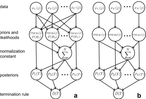
spik-ing MSPRTor simply s-MSPRT. InFig 1it is shown in schematic form to illustrate the flow of

information through the algorithm.

Fig 2shows the time course of a single trial in s-MSPRT which serves to illustrate several key points. First, unlike several other instances of the use of MSPRT in neural decision making, s-MSPRT has its sampling grounded in a physically observable process—spike arrivals—which ties it directly to time. Thus, there is no arbitrary synchronous sampling time of some more

Fig 1. MSPRT in schematic form.Panel a shows the general MSPRT where all theCdata streams contribute to all of theNlikelihoods and thus posteriors, which are then evaluated at a termination stage. Panel b only shows the effective components after all simplifications have been applied.

fundamental continuous-time process, and the decision time emerges naturally in terms of the input data streams. A second observation is that sampling is not uniform; for a given timeT, there are different numbers of observations per channel,si(T), which depend on the firing in that channel. This means theyi(T) are updated at different times, seeFig 2b. Third, while the contributionyi(T) is updated only at spike arrival times on channeli, the log-posterior logPi(T) is updated at the arrival of a spike onanychannel (seeEq 4and black line inFig 2a). Finally, the preceding analysis is quite general; no requirements have been made on the form of the dis-tributions of ISIs (Gaussian or otherwise). In the next two sub-sections, we go on to consider the consequences of using different neurobiologically plausible forms forf0,f.

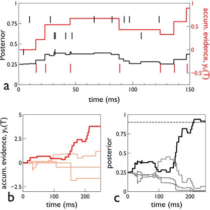
Fig 2. Time course of signals in a single trial of s-MSPRT.The trial is for an s-MSPRT using the gamma distribution, with 4 choices, under the

parameterisation setΩIV(seeMethods). Panel a, shows the spike rasters of the 4 spike trains as small vertical line markers, with that of the preferred channel

in red. This panel also shows the accumulated evidenceyk(T) as a red line graph. Panel b showsyk(T) of all four hypotheses with the preferred hypothesis in

bold red. Panel c shows the posteriors with the preferred hypothesis in black and the others in gray. The threshold is shown by the horizontal dashed line, and was chosen to give a 5% error rate.

Accumulated evidence with exponentially distributed ISIs is

approximately a spike-count

Consider an s-MSPRT with hypotheses that the data is distributed exponentiallyf(x) =λexp

(−λx),f₀(x) =λ₀exp(−λ₀x). Here,λandλ₀are mean instantaneous firing rates, defined by

the inverse of the respective mean ISIμ,μ0. Then, substituting these forms inEq 9.

yiðTÞ ¼

XsiðTÞ

j¼1

log l

l₀ xiðjÞðll0Þ

¼ siðTÞlog

l

l₀ Tiðll0Þ

¼ siðTÞlog

l

l₀ Tðll0Þ þdiðTÞ

ð11Þ

whereδi(T) = (T−Ti)(λ−λ0) and we have used the fact that summing consecutive ISIs just

gives their overall duration (here,Ti). The termT(λ−λ_{0) is hypothesis independent and can}

be absorbed intoB(T) inEq 8. We therefore have

yiðTÞ ¼siðTÞlog

l

l₀ þdiðTÞ ð12Þ

or

yiðTÞ gsiðTÞ; withg ¼ log

l

l₀ ð13Þ

and where the‘error’term defining the degree of approximation isδi(T).

The right hand side ofEq 13is a spike count scaled by a‘gain’g= log(λ/λ₀). This

approxi-mation resembles the expression used by Zhang & Bogacz [17] foryi(T). The difference be-tween the precise form foryi(T) here (Eq 12) and that of [17] stems from them formulating their likelihood function upon discrete Poisson probability mass functions (of spike counts) and us in terms of continuous exponential pdfs (assumed here for ISIs). Nevertheless, up to the approximation inEq 13, we concur with Zhang & Bogacz that, for Poisson-based spike trains (with exponential ISI distributions), the accumulated evidenceyi(T) is given by a (gain-multi-plied) spike count. However, in deriving their result, Zhang & Bogacz started by assuming that

yi(T) comprised the spike count, and then deduced and included a separate gain factor. In con-trast, we have not assumed any a priori form for the total evidence, and have obtained the inte-grated form (counts and gain) inEq 12directly from the general expression for the sum of individual spike contributions inEq 8.

To obtain a better understanding of the spike count approximation inEq 13, use the gain defined there inEq 12to obtain

yiðTÞ ¼gðsiðTÞ þ^siðTÞÞ

where^siðTÞ ¼diðTÞ=gis the error in the spike count. Now consider the spikes immediately

prior to, and afterT. The expectation of the intervals between these spikes andTare equal, and their sum is the mean ISIμ. ThereforehT−Tii= 0.5μand so, for the preferred channel

h^siðTÞi ¼

0:5

g 1

l₀ l

¼ 0:5

g 1e

g

ð Þ

This takes its largest values asg!0, in which caseh^siðTÞi !0:5. There is therefore an upper

bound on the expected error in the spike count to decision on the preferred channel of 0.5.

In general accumulated evidence is not given by a spike-count alone

The exponential distribution is not privileged in its relation toEq 9. Thus, it is possible to ob-tain a closed form forLi(j) for any analytically defined distribution, by substituting a suitably parameterised pair of pdfs forf(x) andf₀(x) intoEq 9. The results for a range of distributions

which may fit ISI data are shown inTable 1. Each distribution has a pair of parametersz,η (not usually the mean and standard deviation of the pdf). Taking two pairs of such parameters

z,ηandz₀,η₀, specifiesf(x) andf₀(x). Substitution inLi(j) inEq 9yields the expressions in

the central column of the table. Each one comprises the sum of a constantg0, and a sum of

products of a coefficient or‘gain’,gi(i= 1,2), together with a simple function of the variable like logxi(j), (logxi(j))2,xi(j)−1. Summation over spikes leads, in all instances, to a term likegi sk(T), which is the analogue of the right hand side ofEq 13; that is, it expresses a‘spike count’ contribution toyi(T).

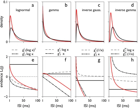
However, there are other terms inLi(j) which depend onxi(j) and which can make a sub-stantial contribution to the development ofyi(T). This is demonstrated inFig 3for a particular set of biologically plausible pdfs and parameterisations,OIV, described in the Methods. Fig3a–

3d, shows the pdfs specified byOIV. In the corresponding panels e-h below,Li(j) is shown per

pdf as a function ofxi(j) (solid red line) as well as the functions for its contributory terms. The termg0is constant (solid black line), the spike count contribution and other non-linear terms

are functions ofxi(j) (dashed and broken gray/black lines). There is clearly a wide variation in non-constant contributions toLi(j). Most notably, the terms linear inxi(j) in the gamma and

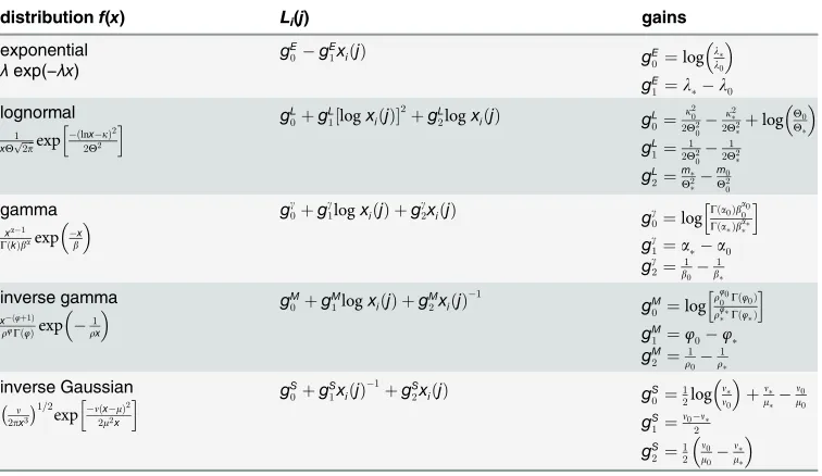
Table 1. Analytic expressions for_‘evidence contributions_’,_Li(j) for a range of distributions.

distributionf(x) Li(j) gains

exponential

λexp(−λx)

gE

0gE1xiðjÞ gE₀¼_log l

l₀

gE

1¼ll0

lognormal

1 xYpffiffiffiffi2pexp

ðlnxkÞ2

2Y2

h i gL0þgL1½logxiðjÞ2þgL2logxiðjÞ gL₀¼ k 2 0

2Y2 0

k2

2Y2þlog YY0 gL

1¼2Y12 0

1 2Y2

gL 2¼ m Y2 m₀ Y2 0 gamma

xa1 GðkÞbaexp _bx

gg

0þgg1logxiðjÞ þgg2xiðjÞ _gg

0¼log Gð

a0Þba₀0 GðaÞba

h i

gg

1¼aa0

gg

2¼b10

1

b inverse gamma

xðφþ1Þ

rφGðφÞexp r1x

gM0 þgM1logxiðjÞ þgM2xiðjÞ1 gM₀ ¼_log r

φ0 0Gðφ0Þ rφGðφÞ

h i

gM

1 ¼φ0φ gM

2 ¼r10

1

r inverse Gaussian

n

2px3

1=2

exp nðxmÞ2

2m2x

h i gS0þgS1xiðjÞ

1_þgS

2xiðjÞ gS₀¼1₂log n

n0 þ n

m

n₀ m0

gS 1¼n02n

gS 2¼12

n0 m0

n

m

The left hand column shows the canonical functional form of the distribution in terms of its‘natural’ parameters. The central column is the evidence contributionLi(j), and the right hand column contains

expressions for the‘gains’in terms of such parameters.

inverse Gaussian, have an apparently disproportionate effect onLi(j). However, as noted earlier in connection with the exponential distribution, when summed over spikes, such terms give an expression which is approximatelygT(for some gaing). If these terms were identically equal to

gT, they may be absorbed into the constant termB(T) inEq 8, and have a null effect on the pos-terior. Thus, assuming the terms linear inxi(j) are a good approximation togT, they will have a very limited influence on the outcome of a decision.

s-MSPRT has a

‘

regular

’

MSPRT counterpart for all ISI distributions

It is instructive to compare the s-MSPRT with a counterpart‘regular’MSPRT with temporally

uniform-sampling; that is, in contrast to neural spike trains, observations are drawn simulta-neously for all channels every time intervalδt(MSPRT as in [10,19,29]). We denote this

Fig 3. The two-parameter families of pdfs (top) and their‘evidence contributions’Li(j) (bottom).Panels a-d show the lognormal, gamma, inverse Gaussian, and inverse gamma pdfs respectively, for the independent variance parameter setΩIV(seeMethods). The‘preferred’and‘null’density functions

(f*,f0) are in red and black respectively. The plots are for ISIs from 1 to 100 ms. For infinitesimal ISIs, the lognormal, inverse Gaussian and inverse gamma tend to zero; for the the gamma the pdf grows up to a bound as the ISI tends to zero. Panels e-f are the corresponding contributionsLi(j) to the accumulated

‘evidence’yi(T) (seeEq 9) and the separate components therein (seeTable 1).Li(j) itself is shown in red, the constant termgD0(D=L,γ,S,M) by the solid

black line, and non-constant terms by dashed-grey and broken-black lines. The horizontal dashed grey line indicates 0 on they-axis.

uniform-sampling variant, u-MSPRT. Note this alternative form, like its s-MSPRT counterpart, is not supposed to be based on observations from an underlying continuous process. Rather, u-MSPRT relies on a fundamentally discrete, sequential process with uniform inter-observation time, but is abstract and does not assume any explicit representation of spike arrivals. Its sole purpose is to provide a‘bridge’from the s-MSPRT to the more usual, uniformly sampled deci-sion processes (which may well assume a continuous time foundation). In this scheme, the dis-tribution-independent formalism developed above is preserved almost in its entirety, withxk(j) interpreted as thejthobservation on channelk, drawn from one of the pdfs describing ISIs. Thus,Table 1applies for all such u-MSPRT, which therefore extends previous results describ-ing the specific form of MSPRT for Gaussian inputs only [10].

In all u-MSPRT variants, the expressions contributing toyi(T) inEq 9now refer to sums up to observations(T) for any channel (instead ofsi(T)) andT=s(T)δt(Ti=T, for alli). With like-lihoods and posteriors thus updated simultaneously for every hypothesis, everyδt, u-MSPRT also takes the form inEq 10and has the structure inFig 1.

We now turn to the comparison between s- and u-MSPRT. For both variants, the decision time is governed by thedecision sample—the number of observations required to reach the threshold. For a given decision, in s-MSPRT the decision sample will depend on the hypothesis which has reached threshold. On average, whenμ<μ0, there will be more observations in a

preferred channel than in one of the null channels; this is observed in cortical sites that supply evidence for decision formation, like the middle-temporal visual area (MT) [30] or the primary somatosensory cortex [24]. We report the expected decision sample with respect to an equiva-lent number of preferred channel observations,hssi, irrespective of the hypothesis crossing the

threshold. For u-MSPRT, all channels are sampled equally frequently but we will, nevertheless, denote the expected decision sample with respect to the preferred channel,hs_ui, in order to fa-cilitate comparison between u- and s-MSPRT.

For s-MSPRT, the decision timeTs

Dis the sum of an integer number of observations,siðTDsÞ,

and a‘residual time’comprising the time fromt0to first spike arrival atti0. For correct

deci-sions, the expected value ofxi(0) is 0.5μ. Thus, the expected decision times for each type of MSPRT are given by

hTs

Di ¼ ðhs

si þ0:5Þm

hTu

Di ¼ hs

uidt

ð15Þ

Notwithstanding the simple formal relations above, the interpretation of decision making by these algorithms, in terms of an overalldecision time, is rather subtle. For s-MSPRT, observa-tions are explicitly determined by spike arrivals, and we will ultimately need to know whether we are we dealing with single or multiple spike trains and, if the latter, how these combine to make ISI-pdfs for algorithm input. These questions are taken up again in the Discussion but, in all subsequent results, we consider processing of an individual afferent spike train as the‘unit of decision making’. All the analyses of ISI statistics described above are, therefore, directly ap-plicable. Further, in previous application of uniform-sampled MSPRT to neurobiological deci-sion making, the parameters were chosen to allowbehaviourallyappropriate decision times [10]. Here, however we wish to examine decision making at the level of spike trains andneural

notwithstanding the problems with interpreting decision times, it is instructive to see what choice of sampling periodδtwould ensure similar decision times. The investigation to answer these questions is largely empirical, but we supply heuristic analysis to give insight into the outcomes.

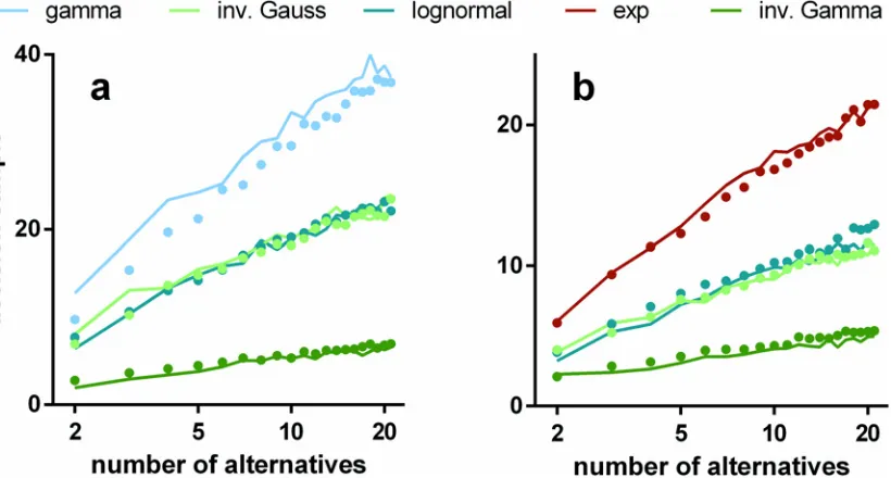
We ran simulations of s-MSPRT as a function of the number of choices or hypotheses,N, for a range of pdfs, and the two parameter setsOIV,OFV(seeMethods). All the simulation

re-sults use trials with an error rate of 5% obtained by iteratively seeking a threshold that satisfied this criterion. Every data point for a particular number of alternatives is the mean over 950 cor-rect, out of 1000 total trials (982 correct for the inverse gamma based s-MSPRT atN= 2 with

OFVinFig 4which is at an error rate of 1.8% as it was not possible to reliably achieve a 5%

error here; this decision task would appear to be too easy to be compromised to this extent). The large trial numbers ensure that estimation of the error rate during threshold determination is sufficiently accurate. For the simulations in this section, the ISIs are drawn from the distribu-tions,ffor the preferred channel, andf₀for the null channels.

The decision sampleshs_siare estimated inFig 4(solid lines). We can consistently interpret these results as decision times becauseμ= 16.5 ms throughout. Then, assuming only the single preferred afferent spike stream,Eq 15implies that 10 observations translates to 165 ms. The solid symbols inFig 4show the comparable decision sampleshs_uifor u-MSPRT. There is clear-ly a very close correspondence between the two sets of mean decision samples across a range of conditions; that is,hsui hs

si. There are two possible exceptions to this; the gamma

distribu-tion with parametersOIVand the exponential withOFV, but even here, the correspondence is

reasonably good. It would appear therefore that, for a given s-MSPRT, there is a u-MSPRT counterpart with the same mean decision sample and error rate. Further, given the provisos above,Eq 15implies that decision times in the two cases will be equal (ignoring the residual

Fig 4. Mean decision samples against number of choices for a range of pdfs, parameter sets, and mechanisms.Each panel shows mean decision sample as a function of the number of choices for a range of pdfs (see legend) and for the two alternative mechanisms: s-MSPRT (solid lines) and u-MSPRT (solid circles). Panels a and b are for the parameter setsΩIVandΩFVrespectively (seeMethods). In the case ofΩFV, the gamma and exponential distributions

are identical and so not reported separately. All data points are the mean of 950 correct, out of 1000 total trials (see text for inverse gamma based s-MSPRT). Error bars are omitted for clarity and are small; the standard error of the mean is typically 2% of the mean.

term 0.5μ) if we assignδt=μ. In the Methods, we develop a heuristic argument to show why there is a close match between the two methods.

s-MSPRT can be more observation efficient than the usual u-MSPRT

ConsiderEq 4. Then, puttingRðTÞ ¼PNk¼1expykðTÞ,Eq 4becomes PiðTÞ ¼

expyiðTÞ

RðTÞ ð16Þ

where,R(T) is a hypothesis independent normalisation constant. The idea, therefore, is to think of the posterior as a‘scaled’version of expyi(T), although this scaling will change at every spike arrival in any channel. This is illustrated inFig 2, in which panels b,c therein show

yi(T) andPi(T) respectively; the notion of scaling is especially clear for the preferred hypothesis. Assuming a small error rate, most decisions will choose this hypothesis, and so the critical fea-ture for the decision time is the trajectory of the integrated evidence therein,y_{(T) (here, and}

henceforth, a‘’subscript denotes quantities on the preferred hypothesis).

In general, the termsL(j) inEq 9contributing toy(T) have similar form whether they are

notionally obtained from spike arrivals or uniform sampling. Therefore, at the level of observa-tions, typical trajectories forP(T) will be similar in u- and s-MSPRT, up to an overall scaling

byR(T). However, even with identically shaped trajectories, the decision sample will depend onR(T) and the threshold in each case. We therefore proceed to examine these quantities.

In evaluatingR(T), we first we note that each contributory termLi(j) to the evidence in the

null hypothesis (in either MSPRT) is likely to be negative, since we expectf(xi(j))/f₀(xi(j))<1.

This, in turn tends to makeyi(T)<0; as an example of this, seeFig 2b. Secondly, suppose we

have taken the same number of observations in both u- and s-MSPRT on the preferred chan-nel. Then, sinceμ<μ0, there will be fewer observations in a null channel for s-MSPRT than

for u-MSPRT because, for the former, they are sampledμ0/μtimes more slowly than those on

the preferred channel, whereas all channels are sampled at the same rate for u-MSPRT. Inci-dentally, note that given the equality of decision samples (with respect to the preferred chan-nel) this means that the total number of scalar observations, summed across all channels, to reach decision is less for s-MSPRT than it is for u-MSPRT. Thence, s-MSPRT is more observa-tion efficientthan its non-spiking counterpart.

There is no single optimal ISI distribution for decision making

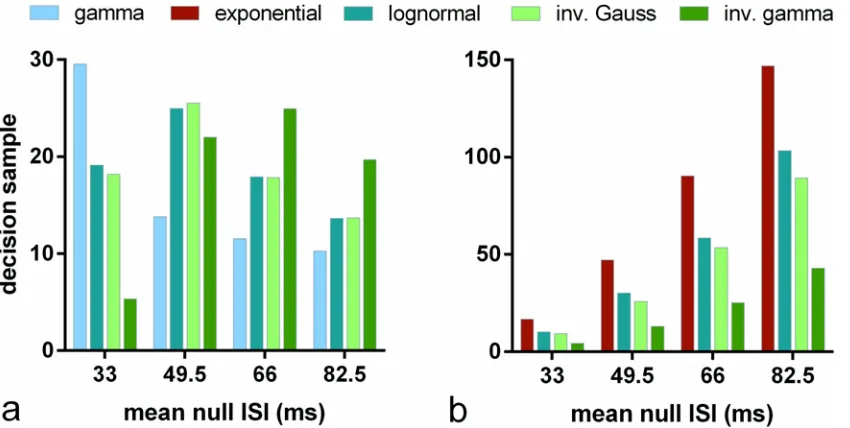
There is a clear distinction inFig 4between the performance of algorithms assuming the differ-ent distributions. Is the rank ordering of performance maintained as we vary the distribution statistics? To explore this we repeated the experiments with s-MSPRT corresponding toN= 10 inFig 4, but with other parameter setsO^IVðm0Þ,O^FVðm0Þ,μ0= 49.5,66,82.5 derived from the

original setsOIV,OFV(seeMethods). The results are shown inFig 5, which also show those for

OIV,OFVfor comparison (μ0= 33 ms).

Fig 5ashows a clear difference in relative performance over the parameter setsOIV,O^IVðm0Þ

In contrast,Fig 5bshows no such variation of performance for the setsOFV,O^FVðm0Þ,

de-fined by their means and variances; the rank order is preserved. The inverse gamma also shows best performance with this parameterisation. In sum, there would appear to be no consistently

‘best’distribution for decision making and that distribution contingent performance varies with the statistics of the data distributions.

Note also that the decision samples under the parameter setsO^FVðm0ÞinFig 5bare much

larger in general than they are for those derived fromOIVinFig 5a. This is because, for

^

OIVðm0Þ, the standard deviation forfandf0does not grow withμ0, whereas it does for

^

OFVðm0Þ, since it is always equal toμ,μ0.

MSPRT is robust under variation of hypothetical distribution

Thus far we have assumed that the underlying statistics of the spike trains are the same as those of the hypothetical distributions (those in the likelihood). In particular, we have assumed that the functional form of the spike ISI distributionsfs

,f0swere identical to their hypothetical

coun-terparts in the decision mechanism,fh

,f0h, (so that no distinguishing superscripth,swas

re-quired). However, in general, the decision mechanism may not‘know’a prioriwhat formfs

,f0s

take. We now ask the question: what effect would an incorrect choice of the pdf formfh

,f0htake

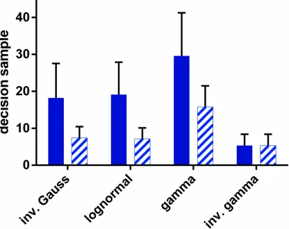
on the decision time? To investigate this we fixed the distributions of ISIs to be inverse gamma, and supplied this data to decision mechanisms (u-MSPRT) based on a variety of pdfs. We used theOIVparameter set for both distribution sets throughout. The results are shown inFig 6by

the pattern filled bars. There is always a change in performance when an‘incorrect’ hypotheti-cal distribution form is used. However, for all the‘incorrectly’established mechanisms, the per-formance is better with the inverse-gamma-distributed data than that when each mechanism

Fig 5. Decision sample in s-MSPRT against mean ISI for range of pdfs and parameter sets.Each bar shows, for the pdf indicated in the legend, the

mean decision sample forN= 10 alternatives, averaged over 950 correct out of 1000 total trials. Panel a used parameter setsΩIV,O^^IVð49:5Þ,O^^IVð66Þ,

^

O^

IVð82:5Þ, panel b usedΩFV,O^^FVð49:5Þ,O^^FVð66Þ,O^^FVð82:5Þ(seeMethods). Each group of bars relates to one parameter set with itsμ0indicated on thex−axis (ΩIV,ΩFVhaveμ0= 33). For the case ofΩFVand anyO^^FVðm0Þ, the gamma and exponential distributions are identical and so not reported separately.

uses observations drawn from pdfs that are the same in the data and the hypothesis test (solid bars inFig 6). Thus, there is no catastrophic decline in performance when using non-matching hypothetical distributions, and performance variation appears more intimately linked to the characteristics of the observations themselves.

Expected total information gain for a decision is constant

It is clear from several of our results that the choice of pdf can make a substantial difference to the decision making performance. However, it is not clear what characteristics of the choice of pdf cause these differences. We might suppose that performance will be a function of how‘far apart’are the distributionsf,f₀and one popular measure of this distance is the

Kullback-Lei-bler divergence (KLD) between two pdfsp(x),q(x) [33], defined by

DðpjjqÞ ¼

Z 1

1p

ðxÞlog₂pðxÞ

qðxÞdx ð17Þ

Fig 6. Decision sample for u-MSPRT when the distributions inthe data were not matched to those tested for.Each bar shows the mean decision sample, forN= 10 alternatives, averaged over 950 correct out of 1000 total trials. The parameter set wasΩIV. The pale, patterned bars are for the case when

the data is always sampled from an inverse gamma distribution, but inserted into mechanisms which test using the distribution indicated on thex−axis (by definition, the bars have equal height for the inverse gamma). The solid bars are for the case when the tested-for distribution matches the true distribution of ISIs, as indicated on thex−axis. Error bars are at one standard deviation.

Here we will use base-2 logarithms, so that results can be reported in bits. Note the KLD is, in general, asymmetric withD(pkq)6¼D(qkp) (although symmetry may occur under some cir-cumstances—e.g.Gaussians with different means and the same variance).

Now letpf,qf₀, then, taking expected values of the per-observation ratios inEq 9with

respect tof

Dðfjjf0Þ ¼ hLiðjÞif 8i;j ð18Þ

The KLD is therefore the mean increase in log-likelihood,yi(T), per observation [41]. Denoting quantities on the preferred channel by, and usingEq 9together with Wald’s identity [42,43], we canfind the corresponding expectation of the accumulated evidence for the preferred hy-pothesis at decision timeTs

D,

hyðTDsÞif ¼ hs

sihLðjÞif ð19Þ

Thus, usingEq 18

hssi ¼

hyðTDsÞif Dðfjjf0Þ

ð20Þ

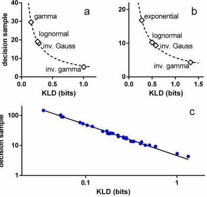
We now turn to an empirical investigation ofEq 20. If the numerator is constant for varia-tion in parameters or pdf, we expect a simple inverse relavaria-tion betweenhssiandD(fkf0). Fig7a

and7bshow that this is indeed true for each of the pdf classesOIV,OFV(μ0= 33 ms), used in

Fig5aand5brespectively. The dashed lines are power law fits and are remarkably good:R2>

0.998, with exponents−0.866,−0.844, forOIV,OFVrespectively. These exponents are almost

-1, as predicted byEq 20and, it would therefore appear that KLD is a good predictor of‘local’ variations in performance under a given parameter set. However, plottinghssiagainstD(fkf0)

for all 32 tests inFig 5indicates a more general result—seeFig 7c, where the log axes emphasise the power law fit over the wide range of the variables. The fitted function is

hs_si ¼4:594Dðfjjf0Þ1:034 ð21Þ

and again, thefit is very good (R2= 0.997). Just as significantly, the exponent is very close to -1, in which case the product of KLD and the decision sample is a constantA

hssiDðfjjf0Þ ¼A ð22Þ

Some indication of why this might be true is supplied by Veeravalli and Baum [44] (see

Methods). This indicates that the‘constant’Adepends only on the error rateand number of hypothesesNaccording to

Að;NÞ ¼ 1

N1

logð1ÞðN1Þ

ð23Þ

(natural logarithm, note that inFig 5,andNarefixed).

Further,Eq 22also has theoretical plausibility grounded in the notion that KLD is a founda-tion of informafounda-tion theory. In fact, in its original formulafounda-tion, it was noted that the KLD gave the meaninformation per observationfor discrimination between two hypotheses about the distribution leading to the sample [33]. This kind of interpretation leads to the KLD also being referred to as aninformation gain. To emphasise this view we writeD(fkf₀)I(f,f₀). Then,

using this, andEq 23, the empirically supported result inEq 22becomes

The left hand side ofEq 24is the product of the mean information gain per observation and the expected number of observations to decision; that is the mean total information required for the decision. Thus,Eq 24states that, for a givenNand, the mean total information for a decision is constant. In this view, the empirically determined constantA= 4.594 bits (Eq 21) is the expected amount of information required to perform a decision among 10 alternatives, with a 5% error rate, given uncertainty in the signals supplied. We now go on to use the result on information conservation to show how the neural refractory period can facilitate decision making and to explain two well known psychophysical phenomena.

The spike refractory period is a benefit, not an impediment, for decision making. In real biological neurons, spikes occupy a finite width and there is a refractory period between spikes which forces a lower limit on the ISI of not less than 1 ms. A popular choice for spike

Fig 7. Mean decision sample for s-MSPRT against KLD.The KLD in all cases isD(f*kf0) (see text). Panels a, b are for decision with the parameter sets ΩIV,ΩFV, respectively, and both useN= 10. The data points are the open symbols and the dashed lines, best fit power laws (nonlinear least squares). In

panel c, the data points shown in blue symbols correspond to all the decision samples inFig 5. The solid line is the best fit power law.

interval generation is the Poisson process for which the ISIs are distributed according to an ex-ponential formfe(x). However,fe(x) has its mode (maximum) atx=xmode= 0 thereby allowing

the unrealistic occurrence of arbitrarily small ISIs. Nevertheless, if the assumption offe(x) dem-onstrated a decision making procedure (e.g.s-MSPRT) with a performance advantage com-pared to other distributions, it could be that real neurons work to ensure their ISI distributions are as close tofe(x) as possible. On the other hand, if assumingfe(x) gives inferior performance compared to distributions for whichxmode>0, the ostensible limitation in neural processing

that is the refractory period may be thought of, instead, as a enhancing feature, since it is this mechanism that has forced a non-zero location of the mode.

To cast light on this issue, consider the results inFig 4b. This shows a comparison of the performance of s- and u-MSPRT assumingfeagainst a range of other distributions withxmode >0 using parameter setOFV. The procedures assuming the exponential distribution clearly

give longer decision times compared to the others. This could be a peculiarity of the choice of the means, but examination ofFig 5bshows otherwise; in all cases the rank ordering of perfor-mance across distributions is maintained and the exponential performs worst. Similarly, the gamma assuming (u-)s-MSPRT performs worst among its cohort underOIV(Fig 5b) while

as-suming distributions with maximum density at infinitesimal values ofx(Fig 3b). ByEq 17, the KLD is determined by the ratio of the entirety of a pair of densities. When the modes of both are greater than 0 they also tend to differ from one another, as it happens in general in neural ISIs under preferred and null conditions, as well as in the rest of our densities under biological-ly realistic parameters (Fig3a,3cand3d). Then, the area under the log-ratio of such densities and thus the KLD between them tend to increase which in turn, byEq 24, improves the ex-pected performance of a decision procedure. All this therefore supports the hypothesis that the existence of a refractory period helps neural decision making by facilitating the contrast of the ISI distributions of simultaneous spike trains.

Information conservation explains Hick’s Law. Hick’s law (sometimes known as the Hick-Hyman law) describes the relation often observed between mean reaction timeTRand the number of alternativesNin choice reaction time experiments with low error rates [35,45,

46]. There are two slightly different variants

TR ¼ alogðNþ1Þ

TR ¼ T0þalogðNÞ

ð25Þ

where thefirst form was that originally proposed by Hick and the second used in more recent applications [47]. The second form is also more plausible as the termT0can absorb irreducible

components of reaction time which originate in some minimum decision time, sensory pro-cessing delay and motor execution. In fact, in tasks where the stimulus-response mapping is too simple or over-learned (e.g.[48,49]), the contribution of the logarithmic,Ndependent fac-tor appears to become undetectable [8].

The use of a log axis forNinFig 4emphasises the fit of the simulation data to laws of this form (all linear regressions of both kinds inEq 25have residualsR2>0.95). Our results are therefore consistent with the psychophysics of choice experiments as expressed in Hick’s law.

Moreover, the information gain perspective is able to explain the general form of Hicks law. Starting fromEq 23, and assuming/(N−1) to be negligible (due to small)

hssiIðf;f0Þ ð1Þ log

ð1Þ

þ logðN1Þ

¼ hðÞ þ ð1ÞlogðN1Þ

withh() = (1−)log[(1−)/]. For given neural distributions,I(f_{,f0) is constant and so}

hs_si ¼aþblogðN1Þ ð27Þ

which is close to the second form of Hicks law (in terms of a decision sample) given inEq 25.

Eq 27is similar to the empirical expression for mean decision time of u-MSPRT obtained by McMillen & Holmes [8]. Through a different method, our expression completes their intuition, confirms the log(N−1) dependence onNand demonstrates this form to generalize to s-MSPRT; both expressions constitute concrete, experimentally testable predictions.

Further, we tested the ability of this theoretical result to quantitatively explain our data, by calculatingI(f,f₀) for the distribution pairs used inFig 4a, and substituted these inEq 26; the

results, together with the original simulation data are shown inFig 8aThere is good agreement with the empirical results.

Information conservation explains Piéron’s Law. There is another widely observed, law-ful relationship in psychophysical experiments which has a long history. Piéron’s law [36,50] is a psychophysical regularity where the simple reaction time to the detection of stimuli across a range of sensory modalities has been found to depend through a power law on the intensity of the stimulus,u. It is also a characteristic of low (≲5%) error rate circumstances [51,52]. Piéron’s law has also been extended to the effect of stimulus intensity on choice reaction times (CRTs) [51,53,54] and to the effect of stimulus separability on CRTs [55]. In terms of the in-fluence of stimulus intensityuon reaction timeTR, Piéron’s law may be written as

TR¼T0þaub; b>0 ð28Þ

Just as inEq 25, the termT0may include components of reaction time which originate in

mini-mum decision time, peripheral sensory delays and motor execution; we are interested only in the main decision making componentau−b.

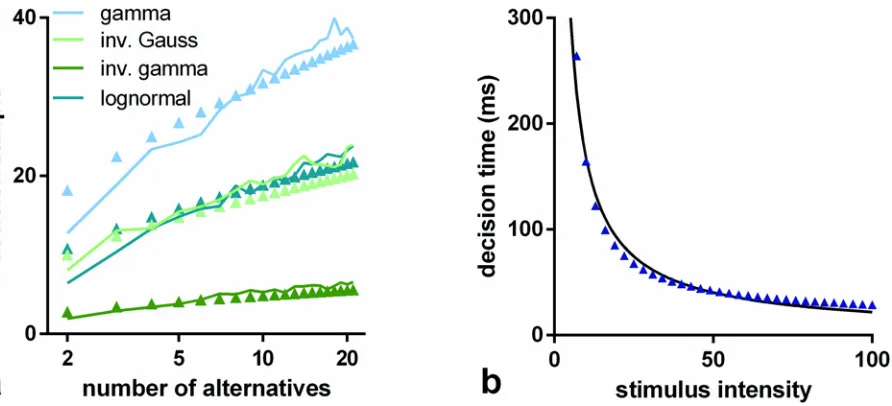
Fig 8. Hick’s and Piéron’s laws from conservation of information.Panel a is a direct counterpart ofFig 4a. The decision samples for s-MSPRT are shown as solid lines and the predictions fromEq 27shown as solid symbols. Panel b shows results of the virtual experiment derived fromEq 30(blue symbols) and a best fit power law (solid black line).

To make the link between this component of Piéron’s law andEq 24we need alinking hy-pothesiswhich describes how neural responses, as firing rates, depend onu; that is we require firing rateras a function ofu. We base this on the study by Muniak et al on firing rates and tac-tile sensation [56]. Here, the task is one of stimulus detection and, while we are interested pri-marily in choices tasks, we take the kind of linking hypothesis developed in that study as indicative of a more general one. Further, we modified the relationr(u) used by Muniak et al [56] to include an explicit baseline firing rater(uθ), whereuθis the sensory threshold.

rðuÞ ¼alog u

uy

þrðuyÞ ð29Þ

The use of a baseline ensures that we are comparing thefiring in the preferred channel with a non-zero null rate; that is we assumeμ0= 1/r(uθ) for afixedf0. Similarly, we assume the pdf of

ISIs in the preferred channel,f_{(u), is parameterised by its mean ISI}μ_{(u) = 1/r(u).}

Then, starting from the decision time relation,TDðuÞ ¼ hs

sim

_{ðuÞ, and using the expression}

forhssifromEq 24, we have TDðuÞ ¼

Að;NÞ

alog u

uy

þrðuyÞ

DðfðuÞjjf0Þ

ð30Þ

To test the validity ofEq 30we ran a‘virtual experiment’, obtaining simulated data points fromEq 30with the following parameterisation, chosen to give firing rates comparable to those in the rest of this article:α= 10,r(uθ) = 10,uθ= 1, 7u100;f,f₀were lognormal

with,σ0= 200 ms,σ= 65 ms; the error rate= 0.05, andN= 2.Fig 8bshows the resulting

the-oretical datapoints (dark blue symbols) and a best fit line of the formTD(u) =au−b. The fit is good, and so it is possible for virtual experiments based onEq 30—derived in turn fromEq 24

—to be described by a Piéron-like law. We infer thatEq 24with a linking relation likeEq 29

could account for Piéron’s lawin vivo.

Discussion

We have shown how arbitrary renewal spike trains may be subject to general Bayes-based se-quential analysis and, when this treatment specialises to the use of log-probability ratios, we ob-tain an instance of the MSPRT. In this spiking MSPRT (s-MSPRT), the data are ISIs, and the sampling times are given by the asynchronous spike arrival times on several parallel channels. The corollary of this is that the posterior, for any hypothesis, is updated at spike arrivals on any channel.

Our analysis of ISI data for neurons involved in a decision task showed that this is not well approximated by a Gaussian. Indeed there is a conceptual problem that the Gaussian admits negative ISIs which is infeasible. On application of s-MSPRT to the most oft-used, realistic ISI distribution–the exponential yielding‘Poisson spikes’–the accumulated evidence,yi(T), up to timeT, is shown to be approximately equal to the scaled count of spikes toT(up to a scaling factor). This grounds previous work by Zhang and Bogacz (2010) [17] whose starting point was theassumptionthat the evidence in this case was given by a (scaled) spike-count. Our re-sult also modifies the rere-sult of [17] showing that, while providing the main source of evidence, for an exponential-based s-MSPRT the spike count needs to be augmented by an additional

‘correction’(δi(T), inEq 12).

accumulated evidence for these was shown to be a spike count with additional terms which, in general, cannot be neglected.

We showed that s-MSPRT is comparable with a uniform sampling counterpart—u-MSPRT

—if the sampling rate of the latter is set to the mean ISI on the preferred channel,μ. However, in making this comparison, we argued that performance is best measured in most cases using the decision sample rather than decision timeper seas the latter requires careful interpretation (see below). The decision samples for s- and u-MSPRT are very close and there is a heuristic ar-gument to be made why this might be so. Nevertheless, s-MSPRT can achieve the same perfor-mance and error rate with fewer observations than u-MSPRT because it doesn’t have to accommodate as many observations from the non-preferred (‘null’) channels; thence, s-MSPRT is more observation efficient than u-s-MSPRT. As with many decision mechanisms (e.g

[8,10,57,58]), both s-MSPRT and u-MSPRT showed a Hick’s law relation between decision sample and number of alternatives.

A key result was that there is no universally optimal distribution for making a decision. The best performance varies with the underlying statistics of the data. However, a decision mecha-nism assuming the exponential distribution shows, in general, an inferior performance com-pared to when assuming other distributions with mode at non-zero ISI. Thus, the spiking refractory period can be viewed as positive feature which aids decision making mechanisms, rather than a drawback which hinders attainment of optimal performance therein.

In most of our simulations, the s-MPSRT was configured to give the best performance be-cause the hypothetical distributions (i.e.those tested for) were matched to those of the data. That is, the decision mechanism was given‘privileged’information about the data. However, this will not normally be the case and we showed a case where this assumption is violated and there is no catastrophic decline in performance.

We showed empirically in our model that the mean total information gain required to make a decision was constant, over a wide range of distributions and parameters. This was supported by some analytic results and so we conjecture that it may be a quite general result. While this result may not sound surprising in isolation, it is remarkable that it emerges empirically in such a precise way from the examination of a variety of conditions with different distributions and parameterisations. This result allowed us to provide a theoretical rationale for Hick’s law and Piéron’s law and a concrete, experimentally testable expression for mean decision time as a function of sensory information content, error rate and number of choices (Eq 24).

Interpretation of s-MSPRT and perceptual decision times

Given this demarcation of processing, there is a wide range of possible neural decision times discernible in perceptual tasks. For example, using high contrast, easily distinguished stimuli in a paradigm designed specifically to tease out the perceptual decision making process, Stanford et al [68] showed that this could occur in as little as 30 ms for a 2-alternative task. However, for the relatively hard to distinguish stimuli in the random dot motion task (RDMT) with 2–4 al-ternatives, neural integration times can be several hundred ms [69,70].

The statistics of the neural data we used here were obtained in a RDMT with stimulus co-herence of 12.8% [30] (seeMethods). In the RDMT-based study of Churchland et al (2008) [69], with stimulus coherence of 12.8%, the mean reaction times forN= 2 andN= 4 were 535 ms and 618 ms respectively. Using estimates of sensory and motor delays of 200–300 ms [60,

71] we would expect corresponding decision times of 285 ± 50ms, and 368 ± 50ms; that is of the order of 102ms. A full behavioural comparison with studies like this is out of the scope of the present article, however, if we convert the sampling times for smallNinFig 4ato decision times usingEq 15, we obtain decision times of the same order as this for several of the distribu-tions, including the lognormal which gave the best fit to the data in [30,31].

Thus far, we have predominantly used a simple version of s-MSPRT based on a single neural input stream on each channel (Fig 1b). In general, however, the theory (leading toEq 10) is neutral regarding the origin of the spikes in each channel—they may derive from a single or multiple neural sources (Fig 1a). We now consider two possibilities for combining the informa-tion across them. In the first, we assume there is some mechanism ofspike superpositionto pool spikes across neurons into a unitary stream before being subject to s-MSPRT. In this case, for large numbers (*100) of contributing streams with arbitrary distributions, the resulting superposition of spike trains has a distribution extremely close to the exponential (albeit with some subtleties of its power spectrum) [72]. Ifμ,μ0are the mean ISIs within each input stream

for preferred and null channels respectively, then theeffectivemeans of the ISIs in the super-posed streams in each channel forMinputs per channel areμ/M,μ0/M. However, assuming a

good approximation to the exponential distribution, the gain,gE

0 ¼logl=l0, remains

un-changed, and so the accumulated evidenceyi(T) is still a spike count which simply scales with

M. This will render shorter decision times and lower error rates, as more information is available.

The second approach works by directly pooling observations overMinputs. It is obtained by directly extending the formalism leading to s-MSPRT to include more inputs than hypothe-ses (C>N). Thus, letxr

kðjÞbe the ISI from ther

th_{spike train of channel setkat timet}j

k;r, and let Tr

k¼maxjft j k;r:t

j

k;rTg, then it is straightforward to show that the analogue ofEq 9is

yiðTÞ ¼

XM

r¼1

XTr_i

j¼1

Lr

iðjÞ; L r

iðjÞ ¼ log

fðxriðjÞÞ f0ðxriðjÞÞ

þBðTÞ ð31Þ

Mechanistically, since the order of summation can be reversed, the operations of integrating likelihood ratio terms over time within a stream, and summing across contributory streams, can be conducted in either order. Since the individual ISI statistics are preserved in each stream, the individualLr

iðjÞare distributed in the same way as their single stream (M= 1)

For largeM, both spike superposition and evidence oversampling may comprisedense cod-ingimplementations (that is, actively engage a large fraction of the relevant neural population).

Sparse codingones could be devised by adding: (a) input spike trains that are weakly- or non-informative for the decision and (b) corresponding distributions in the likelihood functions which make weak contributions to them. All approaches in this study assume that spikes, and functions of spike statistics likeLr

iðjÞ, are independent over different inputs. This is almost

cer-tainly not the case. Studying the net effect of correlations on decision making remains an inter-esting problem since positive correlations among spike trains [73,74] may be detrimental for discriminability, but negative serial ISI correlations may reduce the variability of the signal [75] and help on information transfer [76]. However, our simple independent-input cases, provide a starting point for future models of pooling evidence in these ways. Whatever the details of any ensuing models, the range of single neuron ISI statistics which can yield physiologically plausible decision times will be extended considerably by allowing combination or pooling over many inputs (M>1).

Optimality or sufficiency?

It is often assumed that the brain implements nearly-optimal decision making mechanisms. ForN= 2, u-MSPRT collapses [29] to Wald’s sequential probability ratio test [77]. u-MSPRT is thence optimal in the sense that it minimizes the mean sample size (and decision time) to make decisions at any given error rate; forN>2, it is asymptotically optimal as it minimizes it for vanishingly small error rates [10,29].

Beck et al (2012) [32] have recently shown that decision mechanisms will, in general, be im-plemented in a fundamentally suboptimal way. The main reason they give for this is that the brain does not usually have access to the statistical structure of the task. This was precisely the issue addressed in the Results dealing with robustness. There, the true statistics of the stimuli were supplied by an inverse gamma distribution, but we used incorrect (non-inverse-gamma) hypothetical pdfs for the computation of probability ratios. This mismatch of hypothetical and real, underlying data distributions is inevitable; the real data will never comply exactly with an analytically tractable pdf. Such a mismatch may also occur when the response distribution of sensory neurons changes by learning or adaptation (as in [78–81]) and stops approximating

‘previously trained’hypothetical distributions (although this seems not to happen in MT over RDMT training [82]).

The results in our experiment were that low decision samples were maintained and were, in all cases, lower than those of other mechanisms assuming non-inverse-gamma pdfs used in conjunction with their own, correctly matched data. In this case, therefore a deterministically sub-optimal decision mechanism (in the sense of Beck et al)suffices, because its potentially op-timised variant (here with inverse gamma data matching the test-pdf) is better than

its counterparts.

There is a related argument here which starts with the data. The dataset we used to establish the parametersOIVwas best fit by the lognormal, but MSPRT assuming this distribution does

Neural substrates for s-MSPRT

While the s-MSPRT is grounded in the neuralcommunicationmedium of action potentials (spikes) we have yet to address the way in which specificcomputationsinvolved in mechanisms like s-MSPRT may be performed. Consider first the complete Bayes-based expression inEq 4. This apparently complex form is subject to a mapping onto the basal ganglia—a subcortical group of interconnected nuclei involved in mediating action selection. Thus, Bogacz and Gur-ney (2007) [10] have shown that (at least simplified forms of) the basal ganglia architecture and cortex could implementEq 4when applied to a u-MSPRT, using inputs of Gaussian form. While the original MSPRT was not confined to Gaussian inputs [29], its expression in the form given inEq 4is essential for the mapping to basal ganglia-based architectures. Lepora and Gur-ney [19] have since extended this mapping to much wider range of decision processes (with ar-bitrary type, and numbers of, pdfs). Indeed there are several possible mappings from this form to basal ganglia and associated circuitry [10,19,86]. One possible substrate for a process like the s-MSPRT as a whole therefore, is the basal ganglia and its afferent and target structures.

In all of the anatomical mappings of MSPRT to basal ganglia, the cortex is the locus of the neural representation of integrated evidenceyi(T). Moreover, it has often been assumed that the pdfs delivering input to these integrators are Gaussian (although this is not necessary [17,

19,29,37–39,87]). The integration of Gaussian signals is straightforward if all Gaussian inputs have the same variance; it is simply the product of a gain and a term linear in the (abstract) sig-nal inputLi(j) =xi(j) [7,10,16]. However, the forms foryi(T) resulting from the distributions we consider here can be complex (seeTable 1). We now offer some heuristic arguments to sug-gest how the accumulated evidenceyi(T) might be computed in cortex. In order to ease nota-tion, in what follows we drop indices onxi(j) and represent an ISI generically byx.

One term which occurs several times in defining the accumulated evidence is logx. Now, if

ris the instantaneous firing rate withr= 1/x, then logx=−logr. The transfer function, from currentzto firing ratew, of the simple leaky integrate and fire neuron (LIF) can, under the cor-rect circumstances, approximate the formw=log(z) [88]. Now suppose that the input spikes with ratergive, after low-pass filtering by the membrane, a roughly constant currentz. This will be proportional tor, asz=cr, and so we havew=log(cr) =c0+log(r), withc0=log(c). The constant terms likec0may be absorbed into the termB(T) inEq 8. Thus ifrwas an input to an inhibitory LIF-like neuron, the neuron’s output could form an additive input−log(r) to a sec-ond neural stage which combines the required terms.

Now consider the computation of terms like (logx)2which occur with the use of the lognor-mal distribution. Recall from the narrative immediately followingEq 11, that the sum of ISIs to decision time for theithchannel is justTi, and that this is approximatelyTfor alli. Further, such constant terms makes no overall contribution to the outcome. Thus, a term linear inx, which gives rise to such a sum of ISIs, will have no effect on the decision time (within the ap-proximationT=Ti). We can, therefore, always add a term linear in x to any component with negligible effect on the decision outcome. Thus, we can replace the squared log term by (log

x)2−a2xwith constanta. Usingx= 1/r, this becomesðlogrþa=pffiffirÞðlogra=pffiffirÞ. Each bracket contains a term in−logrwhich we can compute using the procedure described above. The terma=pffiffirinvolves division bypffiffirand could be achieved by shunting inhibition acting on a tonic firing ratea[89–91]. The multiplication of the brackets is also plausible using active dendritic processing [92,93].

From ISIs to behaviour

The s-MSPRT provides a direct link from the information in spike train ISIs to‘neural decision times’which are a component of an overall behavioural decision time or reaction time. Further this link is strengthened by the hypothesis, supported in our simulation work, that the mean total information gain required to make a decision is constant (for a given error rate and num-ber of alternatives). This was a key to providing explanations for Hick’s and Piéron’s laws and provides a direct link from neural signalling to psychophysical observation. We argue that we have laid the foundations for a programme of work in which neural recordings and spike trains’statistical analysis can be made the basis of predictions about behaviour in multi-alter-native choice tasks.

Methods

Choosing probability distributions to model spike data

Fig 9shows the distribution of ISIs (grey histogram) in a macaque MT neuron, from the study by Britten et al [30,31] using the RDMT. In this task, the monkey is typically shown two eccen-tric targets and then a kinematogram composed of dots in which a given percentage of them (the so-called‘coherence’) move towards one of the targets, while the others move randomly. The animal is rewarded if it saccades towards this target from a gaze fixation point [30,94]. The RDMT is therefore a perceptual decision making task of the kind we envisage being solved by a mechanism like the one proposed (s-MSPRT).

Each panel ofFig 9shows the best fit (using the method of moments) of a pdf to the experi-mental data in the histogram. Data is assumed to come from single neurons and thus to be drawn from one such pdf; the implications for multiple neurons are considered further in the Discussion. All the pdfs are from the exponential family. The choice of putative distributions had the following rationale. The Gaussian, while an oft-used choice in more abstract (e.g. ma-chine learning) approaches, cannot, in principle, be a genuine candidate for ISIs as there will al-ways be a negative tail to the distribution which is physically implausible (there is no such thing as a‘negative ISI’). However, it might be argued that this tail is, in most realistic cases, very small and that it can be neglected. We tested this possibility with real data sets (including that shown inFig 9). The exponential distribution of ISIs leads to spike trains following a Pois-son process—another popular choice for spike train analysis. This time, while the distribution satisfies the positivity requirement, it does not satisfy the requirement for excluding arbitrarily small ISIs due to a neural refractory period. In order to achieve this the distribution must have positive mode as well as lying wholly in the positive half-plane. In addition, we require that the pdf is, in general, positively skewed which matches the general shape observed in ISI data. These requirements are satisfied by suitable parameterisations of the other four candidate dis-tributions: lognormal, gamma, inverse-Gaussian and inverse gamma.

The inverse Gaussian and lognormal appear to be the best fit to the single data set inFig 9. In contrast, note the large (implied) negative tail of the Gaussian, which could certainly not be neglected in using it to sample from for a decision process. However, aside from these qualita-tive observations, we sought to quantify the fitting process by repeating it with several data sets, and using two‘goodness of fit’metrics, the Kolmogorov-Smirnov and Anderson-Darling (see