Characterization of the Binding Properties of Molecularly Imprinted Polymers

This is a repository copy of

Characterization of the Binding Properties of Molecularly

Imprinted Polymers

.

White Rose Research Online URL for this paper:

http://eprints.whiterose.ac.uk/85148/

Version: Accepted Version

Book Section:

Ansell, RJ (2015) Characterization of the Binding Properties of Molecularly Imprinted

Polymers. In: Mattiasson, B and Ye, L, (eds.) Molecularly Imprinted Polymers in

Biotechnology. Advances in Biochemical Engineering/Biotechnology, 150 . Springer

International Publishing , 51 - 93. ISBN 978-3-319-20728-5

https://doi.org/10.1007/10_2015_316

[email protected] https://eprints.whiterose.ac.uk/

Reuse

Unless indicated otherwise, fulltext items are protected by copyright with all rights reserved. The copyright exception in section 29 of the Copyright, Designs and Patents Act 1988 allows the making of a single copy solely for the purpose of non-commercial research or private study within the limits of fair dealing. The publisher or other rights-holder may allow further reproduction and re-use of this version - refer to the White Rose Research Online record for this item. Where records identify the publisher as the copyright holder, users can verify any specific terms of use on the publisher’s website.

Takedown

If you consider content in White Rose Research Online to be in breach of UK law, please notify us by

Molecularly Imprinted Polymers

Richard J. Ansell

School of Chemistry, University of Leeds, Leeds LS2 9JT, United Kingdom

Abstract

The defining characteristic of the binding sites of any particular molecularly imprinted material is heterogeneity: that is, they are not all identical. Nonetheless, it is useful to study their fundamental binding properties, and to obtain average properties. In particular, it has been instructive to compare the binding properties of imprinted and non-imprinted materials.

This chapter begins by considering the origins of this site heterogeneity. Next, the properties of interest of imprinted binding sites are described in brief: affinity, selectivity, and kinetics. The binding/adsorption isotherm, the graph of concentra-tion of analyte bound to a MIP versus concentraconcentra-tion of free analyte at equilibrium, over a range of total concentrations, is described in some detail. Following this, the techniques for studying the imprinted sites are described (batch binding assays, radioligand binding assays, zonal chromatography, frontal chromatography, calo-rimetry, and others). Thereafter, the parameters which influence affinity, selectivi-ty and kinetics are discussed (solvent, modifiers of organic solvents, pH of aque-ous solvents, temperature). Finally, mathematical attempts to fit the adsorption isotherms for imprinted materials, so as to obtain information about the range of binding affinities characterizing the imprinted sites, are summarized.

1. Properties of molecularly imprinted binding sites

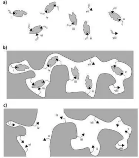
pre-served in the macromolecular material after polymerization (Figure 1b). Pro-cessing of the material (e.g. by grinding and sieving), removal of the template, and exchange of the polymerization solvent with a different solvent to study the bind-ing properties, can all lead to further heterogeneity by damagbind-ing bindbind-ing sites, sites collapsing on template removal, and locally variable swelling/collapse of the polymer in a different solvent (figure 1c).

The binding site heterogeneity is usually acknowledged at least in so far as au-thors discuss ‘specific’ and ‘non-specific’ binding to imprinted materials. At the simplest level, we might consider sites arising from any form of monomer-template complex in the pre-polymerisation mixture (i-vi in figure 1) to be ‘specif-ic’μ these are expected to have a higher affinity for the template (and similar struc-tures), and to be more selective in not binding dissimilar ones (due to ‘the precise arrangement of the functional groups’ and ‘shape selectivity’). Sites arising from free, non-complexed monomer in the pre-polymerisation mixture (vii and viii in figure 1) are proposed to give ‘non-specific’ sitesμ these are expected to have low-er affinity for the template and to bind othlow-er species indiscriminately, just as a polymer with randomly arranged functional monomer (e.g. a non-imprinted poly-mer, prepared in the absence of template) would be expected to behave. However, whilst this simplistic dichotomy between ‘specific sites’ and ‘non-specific sites’ (or ‘imprinted sites’ and ‘non-imprinted sites’) can be useful, it certainly does not capture the full picture, which is of a continuous spectrum of sites from weaker binding, less selective, to stronger binding, more selective.

The diversity of species in the pre-polymerisation mixture will be even greater than suggested in Figure 1a if there is more than one type of monomer present, or if the monomer or the template are capable of interactions with the cross-linker, or if ‘clusters’ of template are present [1-4]. The thesis that the pre-polymerisation species (Figure 1a) are precisely replicated in the polymerized material (Figure 1b) is probably naïve, several works having suggested that these structures change during the course of polymerization [5]: however, the broader principle that diver-sity is preserved or enhanced is certainly valid (e.g. due to the polymeric chains being folded in different ways around different sites, ‘outer sphere’ interactions for each site will be different).

Although the model in Figure 1 particularly illustrates the case for non-covalent imprinting of organic monomers, which polymerise into cross-linked chains, the principle is applicable to all forms of imprinting:

- Stoichiometric non-covalent/covalent/semi-covalent/metal-mediated imprint-ing: although these strategies all involve entirely (or almost entirely) 1:1 complex-es of monomer and template, such that there are (in theory) no free monomers, nor any 2:1 or higher complexes, diversity will still be generated due to the different ‘outer-sphere’ interactions in the polymerized material, different site accessibility, plus changes due to site damage in polymer processing, site collapse, and swell-ing/collapse of the polymer after solvent exchange.

- Sol-gel imprinting: the monomeric species may form more than one covalent bond with the cross-linker, the cross-linker may be multivalent, and the polymeri-sation ionic rather than free-radical, but the principles of figure 1 remain. The cross-linked gel is an amorphous material, even if it is inorganic, without crystal-line form, so the structure is just as heterogeneous.

homo-geneous surface and the monomers form a monolayer, then the difference in ‘out-er-sphere’ environments of the binding sites will certainly be limited. However, even with stoichiometric monomer-template interactions and a monolayer ap-proach, there will still be differences in the exact orientation of functional groups on the surface and defects in the structure.

- Pre-polymer imprinting: polymer chains can be ‘fixed’ in the presence of a template by phase-inversion precipitation [6] or solvent evaporation [7] the chains are cross-linked physically but not chemically. These approaches are closely relat-ed to ‘bioimprinting’ in proteins whose structure is ‘frozen’ by lyophilisation or chemical cross-linking in the presence of a template[8]. A range of structures will be present initially as the template interacts with the linear polymer, and the heter-ogeneity of folded structures formed during precipitation will be no less than when the polymer chains cross-link covalently.

A great deal of effort has been invested in reducing the heterogeneity of the pre-polymerization mixture for non-covalent imprinting as represented in figure 1a, by studying the template equilibria to optimize the template ratio [9], by choosing/creating new monomers such that the monomer-template interaction is as strong as possible [10-15], and at the simplest level by choosing a solvent in which the interactions are strongest. However, diversity in the binding sites cannot be avoided, for the same reasons that it is present even in covalent imprinting.

For some applications, some binding site diversity (for example, a range of dif-ferent binding site affinities) may be useful [16] however in most applications it is considered a hindrance (for example in zonal chromatography, where it leads to the tailing of chromatographic peaks and consequently poor column efficiency and resolution), and it is perceived by the wider scientific community as a limitation. Certainly, in order to design imprinted materials for specific applications, it is es-sential to have an understanding of the binding site heterogeneity and how it aris-es.

When characterizing the binding properties, there are three properties of partic-ular interest:

- Binding site affinity: the binding/unbinding of analyte to/from the imprinted binding sites can be represented as an equilibrium:

free analte binding site abound analyte (1)

Where Ka is the association constant (in mol -1

L), and if all sites were identical then Ka might be expressed as

a _emptybound _d (2)

where Kd is the dissociation constant (in mol L-1), nbound is the mols of bound

analyte, F is the concentration of free analyte in solution (in mol L-1) and nempty is

equivalent (as outlined above), each site (in the same material) will have a differ-ent Ka. The quotient (nbound / (nempty × F)) will change even as the total amount of

analyte changes. Moreover the number of empty binding sites is not a parameter that can be readily measured, hence the calculation of association constants for a MIP polymer is not straightforward (see sections 2 and 5). Instead, the binding under a specified set of conditions is usually expressed simply as nbound, or as

%bound (nbound/nanalyte×100%, where nanalyte is the total mols of analyte present in

the experiment), or as a distribution ratio D (in L g-1)

bound M�P

free (3)

where B is the concentration of bound analyte (in mol g-1), MMIP is the mass of

MIP polymer (in g), V is the volume of solution in which the material is incubated and nfree is the amount of free analyte in solution (in mol) such that

analyte bound free (4)

- Binding site selectivity: the presence of ‘imprinted sites’ is usually verified by comparing an imprinted polymer with one made under the same conditions but in the absence of template (the non-imprinted polymer, NIP). One commonly calcu-lated parameter is the imprinting factor, IF, best defined as the ratio of the distri-bution ratio for a particular analyte, under a particular set of conditions, on the im-printed polymer, to the distribution ratio for the same analyte, under identical conditions, on the NIP:

M�P N�P

M�P M�P N�P N�P

bound M�P free M�P

bound N�P free N�P (5)

where the volume V is the same for the MIP as for the NIP, and MMIP is the

same as MNIP. The IF should have a value greater than 1, the higher the value the

competitor _{competitor M�P}analyte M�P _{competitor M�P}analyte M�P analyte M�P_{competitor M�P} (6)

The selectivity factor, , should have a value greater than 1, and high values of for a range of competitors provide evidence of selectivity.

- Binding/unbinding kinetics: The binding/rebinding process can be represented as

free analte binding site bound analyte (7)

where the rate constant k1 (in mol -1

L s-1) is such that

bound

empty (8)

The unbinding process is represented as

bound analyte free analte binding site (9)

where the rate constant k-1 (in s-1) is such that

empty bound

bound (10)

from which it follows that, under conditions of dynamic equilibrium

bound empty (11)

and so

bound

empty a d (12)

Unfortunately, just as every different site on the imprinted material has a dif-ferent association constant Ka, so it will also have different on (k1) and off (k-1)

rate constants. Nonetheless, under a specific set of conditions it is possible to measure effective constants, Ka, k1 and k-1. The rate constants for binding and

2. The binding/adsorption isotherm

2a. Collecting experimental data

Although frequently the binding of analyte is reported as nbound, % bound or D

under a single set of conditions, this is a poor way to characterise MIP binding. Each of these values will vary, even for the same combination of polymer, analyte and solvent, if nanalyte, V or MMIP are changed. This will effect both the binding to

MIP and to a control polymer, and binding of competitors, such that IF and will also change with nanalyte, V and MMIP [18,19]. Moreover, comparison between

dif-ferent MIPs is extremely difficult if binding is only recorded under a single set of conditions. Both Allender et al. [20] and Horvai et al. [18,19] have blamed the common use of single-point characterization for the confusion of many research-ers from other fields when approaching the molecular imprinting literature.

According to both of these groups (and the current author), a far more useful way to characterize analyte binding is to measure/calculate values of the bound concentration B and free concentration F for a fixed amount of polymer and range of concentrations of added analyte: the graph of B versus F yields a binding iso-therm as illustrated in Figure 2. This can be achieved in different ways, the sim-plest being to vary nanalyte while V and MMIP are kept constant, then, once

equilibri-um is achieved, measure F and calculate B. This method is commonly referred to as a batch binding or batch rebinding assay – it and other methods to derive the isotherm are discussed in section 3. Using B = nbound/ MMIP and equation 4, B can

be calculated from nanalyte and F:

analyte free

MIP

analyte

Fig. 2. A typical standard equilibrium bound (nmoles/mg)/free ( M) isotherm for a molecularly

imprinted polymer (MIP) and a control non imprinted polymer (NIP). In this example, the data describe binding isotherms for a propranolol imprinted poly(ethyleneglycoldimethacrylate co methacrylic acid) MIP and its corresponding NIP. Polymers were prepared by precipitation polymerisation[21]. Figure reproduced with permission from [20].

The data points may be connected by curves as shown in Figure 2, either em-pirically or based on a particular model of the type of binding sites present, as dis-cussed in section 2b. ‘Isotherm’ refers to the temperature being kept constantμ binding will change with temperature so it is important that all measurements are made at a constant temperature (and that the temperature is reported), just as it is important that the solution conditions (solvent, buffer, pH etc.) are also the same for all points on the experimental isotherm.

The experimental isotherm should ideally be derived from as many measure-ments, covering as wide a range of nanalyte as possible. The isotherm for a MIP is

not expected to be linear: rather, it usually flattens off at high F as in figure 2. This indicates saturation: all of the binding sites on the MIP are occupied so that B can increase no further even if more analyte is added to solution. The curvature of the binding isotherm can only be properly visualized if a wide enough range of con-centration is studied.

Commonly, binding to a NIP (made under identical conditions and with identi-cal constitution to the MIP except for the absence of the template molecule) is used as an indicator of non-specific binding (though this model is slightly naïve, as discussed in section 1). The NIP is considered to possess functional groups ran-domly arranged on its surface, and these interact with the analyte and cause it to bind to some extent, although (hopefully) more weakly than it does to the MIP. The difference in binding to the MIP and the NIP is attributed to specific binding i.e. the additional binding which occurs due to the presence of selective imprinted sites. For applications where selectivity for the analyte is important, efforts are usually made to maximize the specific binding i.e. the difference between the MIP and the non-imprinted control.

For consistency and ease of comparison, it is important that the isotherm is in-deed expressed as a plot of B vs F. Other representations (e.g. with %bound or nbound on the y-axis, and/or with the total concentration of analyte nanalyte/V, or just

ntotal on the x-axis) are less useful for direct comparison, and unhelpful if

parame-ters such as MMIP or V are not given. Whereas F may indeed be similar to the total

concentration of analyte when the %bound is very small (because binding is ex-tremely weak and/or because MMIP is small compared to the amount of analyte),

these quantities will be different when %bound increases, and the visualization of B vs F is far more useful than B vs total concentration as we shall see below.

One benefit of expressing the isotherm as B vs F and fitting data to an empiri-cal curve is that we can draw, on the same graph, a straight line to represent the range of possible values for B and F given particular values of nanalyte, V and

y-intercept is the limiting value of B if all the analyte binds while its x-intercept is the limiting value of F if none of the analyte binds.

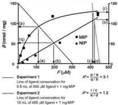
For example figure 3 combines the isotherm with two straight lines represent-ing different combinations of nanalyte, V and MMIP. Where the straight line intersects

the empirical isotherm gives the expected values of B and F under these condi-tions. Under the theoretical conditions of experiment 1, the MIP is expected to give B ~ 92 nmol mg-1 and F ~ 110 mol dm-3 and the NIP B ~ 52 nmol g-1 and F ~ 195 mol dm-3. These values correspond to D for the MIP ~ 0.84 mL mg-1 and for the NIP ~ 0.27 mL mg-1, giving an IF of ~3.1.

Fig. 3. An example of how distribution ratio (D) and imprinting factor (IF) are influenced by experimental parameters of ligand concentration, incubation volume and polymer mass. In Ex-periment 1, 0.5 ml of 300 M ligand and 1 mg of polymer results in an IF of 3.1 whereas in Ex-periment 2, for 1 mg of the same MIP and NIP, a larger volume (10 ml) of 450 M ligand solu-tion gives an IF of 1.2. Figure reproduced with permission from [20].

Under the theoretical conditions of experiment 2 (in figure 3) where nanalyte is

much higher than experiment 1, the MIP is expected to give B ~ 128 nmol mg-1 and F ~ 410 mol dm-3 and the NIP B ~ 110 nmol g-1 and F ~ 420 mol dm-3. These values correspond to D for the MIP ~ 0.31 mL mg-1 and for the NIP ~ 0.26 mL mg-1, giving an imprinting factor of ~1.2. Thus, the model described in figure 3 helps illustrate and explain how, as nanalyte increases relative to MMIP:

- nbound increases but, due to the curvature of the MIP isotherm, not as rapidly

as nanalyte. Hence

- DMIP, falls. Whilst

- DNIP does not change so much, because the isotherm for the NIP is more

line-ar. Hence - IF decreases.

re-flect the conditions under which the MIP is intended to be used in a real applica-tion.

2b. Fitting the experimental data to a model

Where sufficient data points are collected and the errors are shown to be suffi-ciently low, data points on the binding isotherm may be fitted to a curve which can be either empirically based, or based on a theoretical model of the number of bind-ing sites and their bindbind-ing affinities. In figure 2, the isotherm is fitted to an arbi-trary exponential function B=129.7(1-e-0.01132F).

When the flattening of the curve at high values of F is clear, as it is in figure 2, it is possible to measure two empirical parameters Bmax, which is the value of B

when all of the binding sites are occupied and must usually be extrapolated, and Kd which is the value of F (free analyte concentration) at which B = 0.5× Bmax.

From figure 2, values are obtained of Bmax = 130 nmol mg-1 and Kd = 61 M.

Al-lender et al. [20] have suggested that Bmax and Kd should be used commonly as a

measure of the affinity of a MIP, and have conducted a meta-analysis of data on 47 MIPs from different publications between 2004 and 2008, which suggests that

Bmax values commonly range between ~1 nmol and ~ 1 mol per mg of polymer,

while Kd values commonly range between ~1 M and 8 mM.

Model name

Equation Classes of sites? Linearises? Saturates?

Langmuir

max

d

One,

homogene-ous Yes Yes

Bis-Langmuir max

d

max

d

Two No Yes

Tri-Langmuir max

d

max

d

max

d

Three No Yes

Freundlich Continuous distri-bution – infinite number of v weak sites decaying to few v strong ones

Yes No

Langmuir-Freundlich max

Gaussian distribu-tion with clear maximum.

Yes, but re-quires esti-mation of

Bmax

Yes

Table 1. Models used to fit experimental MIP adsorption isotherms.

The simplest (and most optimistic) model used has been the Langmuir iso-therm, which assumes that all binding sites are identical, with a binding (associa-tion) constant Ka and dissociation constant Kd =1 / Ka. From the equation in Table

1, it may be seen that when F=Kd then B = 0.5×Bmax. Thus the empirical constants

Bmax and Kd described above are interpreted, in the Langmuir model, as the

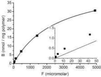
densi-ty of binding sites and the dissociation constant of those sites. Experimental values of B/F may be fitted to the isotherm using graph-fitting software, for example fig-ure 4 shows data for caffeine binding to a caffeine-imprinted polymer fitted to the Langmuir isotherm using OriginProTM. Values are obtained from the data fit of Bmax=(47±1) nmol g-1 and Kd = (2650±140) M.

Prior to the availability of simple graph-fitting software, various approaches were used in which the Langmuir isotherm was linearized, to give a straight-line equation where y and x correspond to combinations of B and F. Best known of these is the Scatchard plot, where B/F is plotted against B. The Langmuir equation can be rearranged to show

d

max

d (14)

Hence, a plot of B/F against B should be a straight line with gradient -1/Kd and

y-intercept Bmax/Kd. Figure 5 shows the corresponding representation of the same

data as in figure 4:

Fig. 5. Scatchard plot for binding data for a caffeine-imprinted MIP determined by radioassay using the binding of 14C-caffeine probe, same conditions as figure 4 [23].

The data do not fit a straight line, confirming the inappropriateness of the Langmuir model in this case. However, it does appear (and is frequently observed with MIPs) that the Scatchard plot could be fitted with two separate straight lines – one line passing through the 7 points at lowest B values and another through the 3 points at highest B values. This approach is often taken, with the gradients and intercepts of the two lines being used to derive two sets of Bmax and Kd values –

one attributed to ‘strong’ binding sites and the other to ‘weak’ binding sites. How-ever, this yields poor estimates of the parameters (see reference [24]).

The bi-Langmuir isotherm (table 1) is a model with two classes of binding sites (one with Bmax1 and Kd1, the other with Bmax2 and Kd2). This expression cannot be

linearized in any combination of B and F, but non-linear graph-fitting software can be used to fit data. It was used initially by Mosbach et al. to fit isotherms ob-tained in MIP radioligand binding assays [25,26] and has been very widely ap-plied since (e.g. [27-30]). Figure 6 shows the same data as in figure 4, fitted to the bi-Langmuir isotherm: the fit is much better, particularly at low F values. The fit-ted parameters are Bmax1 = (1.09±0.16) nmol g-1 and Kd1 = (30.4±10.9) M, Bmax2 =

Fig. 6. Experimental B-F data for a caffeine-imprinted MIP as in figure 4 [23]. Data fitted to bi-Langmuir isotherm using OriginProTM. Inset magnifies data at low F.

The bi-Langmuir model is appealing, as it reflects the simplistic picture of spe-cific, imprinted sites (the stronger binding sites, of which there are but few, in this case described by Bmax1and Kd1), and the non-specific, non-imprinted sites (the

weaker sites, of which there are relatively many, in this case described by Bmax2and Kd2). Variations such as tri- (table 1) and tetra-Langmuir isotherms can

be created by adding third and fourth terms to the equation, describing additional classes of sites: however it is important to acknowledge that adding additional pa-rameters will inherently improve the fit between any model and data, and the in-clusion of these additional parameters is only justified if the improvement in the fit is statistically significant as proven, for instance, by use of an F-test [22].

Models with two, three or even more classes of sites remain an oversimplifica-tion of the real situaoversimplifica-tion in most cases, where there is likely to be a broad range of binding sites, each with slightly different conformations of functional groups and slightly different arrangements of polymeric chains, so that a more-or-less contin-uous range of binding sites with varying Kd values is more realistic.

Fig. 7. Experimental B-F data for a caffeine-imprinted MIP as in figure 4 [23]. Data fitted to Freundlich isotherm using OriginProTM. Inset magnifies data at low F.

Although the Freundlich isotherm fits poorly in this case, it has been fitted more successfully to data from other MIPs, being used first by Guiochon et al. [29], and subsequently by the groups of Shimizu [31-33], Spivak [5] and many others. However, it does have some disadvantages, in comparison with other bind-ing models [33]:

- it does not allow for binding saturation (i.e., however high F is increased, the isotherm predicts that more analyte can bind to the polymer indefinitely)

- the distribution of binding sites underlying the model is an exponentially de-caying distribution, which predicts an infinite number of binding sites with Kd=0.

One advantage of the Freundlich isotherm is that it can be linearized, as in equation 15, such that the graph of logB vs logF has gradient m and intercept log A:

log log log (15)

Fig. 8. Log-log plot of B-F data for a caffeine-imprinted MIP as in figure 4 [23]. Data fitted to straight line using OriginProTM.

The fourth commonly-applied model is the Langmuir-Freundlich isotherm (ta-ble 1) which was first applied to MIP binding data by Shimizu et al.[34], and has since been used by the groups of Martin-Esteban [35-37], Tovar [27], Diaz-Garcia [38] and many others. As in the Freundlich isotherm, a (dm3 mol-1) and m (di-mensionless) are empirical constants, which may be related to the binding site densities and dissociation constants, but non-trivially (section 5). When m = 1, the equation reduces to the Langmuir isotherm, whilst when F is extremely small, it reduces to the Freundlich isotherm (with A = Bmax × a). The equation is equivalent

to the Hill equation, used in biochemistry, in which the coefficient m indicates the co-operativity of binding (m>1 indicates positive co-operativity, while m<1 indi-cates negative co-operativity). The Langmuir-Freundlich isotherm does saturate, such that Bmax is the maximum density of bound analyte at very high F. It can also

be shown that the concentration of free ligand at which B = 0.5×Bmax is given by

Kd = (a)-1/m.

Fitting the data from figure 4 to the Langmuir-Freundlich isotherm yields Bmax

(60.9±3.2) nmol mg-1, a = (7.69±0.87)×10-4 dm3 mol-1 and m = 0.845±0.021, hence Kd = 4840±570 mol dm

-3

. The fit is better than for the Freundlich isotherm though not, in this case, as good as for the bi-Langmuir isotherm (figure 9). The Langmuir-Freundlich isotherm also has the advantage that it may be linearized in the form

ln

max ln ln (16)

Since Bmax is unknown, it must be estimated from the B-F data and

systemati-cally optimized until the plot of ln(B/(Bmax-B)) vs lnF gives the best straight line

possible.

3. Methods for the characterization of imprinted binding sites

3a. Batch binding studies

The simplest possible experiment to characterize the properties of an imprinted material involves incubating a known mass of material (MMIP, in g), with a known

quantity of analyte (nanalyte, in mol) in a known volume of solvent (V, in L or mL).

Once equilibrium has been reached (minutes, or hours, depending on the nature of the material), some will have bound to the material and some remains free in solu-tion (equasolu-tion 1). The material is separated from the solusolu-tion and the free concen-tration F remaining in solution is measured. It is usually simpler (and more relia-ble) to measure F (from which nfree may be calculated) rather than B (which can

then be calculated using equation 13).

In early work, Wulff et al. performed batch-binding experiments e.g. with

ra-cemic 4-nitrophenyl-mannopyranoside binding to a 4-nitrophenyl-

-D-mannopyranoside-imprinted vinylphenylboronic acid-co-DVB polymer. [39]. However, the batch binding method was first applied to derive MIP adsorption isotherms by Shea et al. [40] but has been used subsequently in hundreds of publi-cations, inter alia [27,35,38,41-47].

hence it is essential that the MIP is washed exhaustively before characterization. To check for the absence of error due to template bleeding, a control experiment where MIP is incubated in the assay solvent with nanalyte=0 should be conducted. In

all cases, experimental procedures should be thoroughly described and where pos-sible, uncertainties should be estimated and propagated in the calculation of B and F, and shown as error bars on the isotherm.

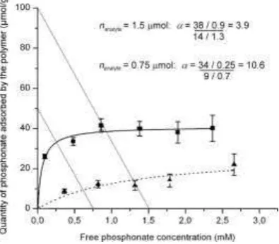
Frequently the isotherms on the MIP and an equivalent NIP are compared, as in figure 2. It was shown above that consideration of the MIP and NIP isotherm ex-plains why IF is dependent on the ratio of analyte to polymer. Batch binding ex-periments can also be applied to derive selectivity factors. The MIP is incubated together with the target analyte, and an equivalent experiment is set up with a competitor, under identical conditions. Measurement of the free concentrations of analyte, and of competitor, then allows calculation of the selectivity factor via equation 6. Consideration of a wider range of data for a target analyte and a com-petitor, presented as binding isotherms as in figure 10, allows us to see why also is dependent on nanalyte, and may increase for lower ratios of nanalyte to MMIP

Fig. 10. An example of how distribution ratio (D) and selectivity factor ( ) are influenced by ligand concentration. Data are for pinacolyl methylphosphonate (PMP, squares) and diphe-nylphosphinic acid (DPPA, triangles), incubated in 1 mL of toluene with 15 mg of PMP-imprinted MAA-co-DVB. Lines of ligand conservation drawn for nanalyte = 1.5 mol and 0.75

mol. For the higher nanalyte, DPMP = 42 mL g-1 and = 3.9, while for the lower nanalyte, DPMP = 136

mL g-1 and = 10.6. Figure adapted with permission from [47].

Fig. 11. Kinetic batch rebinding of hemoglobin (0.4 mg ml-1) on hemoglobin-imprinted chitosan beads (0.5 g in 25ml buffer). Concentration determined after sedimentation of beads by absorb-ance at 280 nm. Figure reproduced with permission from [41].

The example in figure 11 is of extremely slow rebinding kinetics – attributable to the large size of the template (hemoglobin) which has been imprinted within large polymer particles. In contrast, kinetic batch binding studies of a small mole-cule binding to a MIP can show much faster kinetics (e.g. for chloramphenicol binding to a chloramphenicol-imprinted diethylaminoethylmethacrylate-co-EDMA polymer particles in THF, binding was observed to be essentially complete within 2 min [38]).

3b. Radioligand binding studies

A variation on the batch binding assay is where, rather than incubating polymer and analyte in the assay solvent, a mixture of polymer, analyte and radiolabelled probe are incubated in the assay solvent. When the radiolabelled probe is simply an isotopic variant of the analyte, it may be assumed that the probe binding direct-ly reflects the anadirect-lyte binding (equation 17, where nfree probe is the amount of free

radiolabelled probe in mol, and nprobe is the total amount of radiolabelled probe in

the assay, in mol).

free analyte

free probe

probe (17)

nfree probe can be measured, after separation of the solution from the polymer, by

scintillation counting, and nprobe can be quantified by a control with no polymer.

Thereafter equations 3 and 4 are used to derive B and F: the amount of probe is considered to be insignificant such that the total amount of analyte, nanalyte, is just

equal to the unlabeled amount. An advantage of this approach is that it is adapta-ble to a huge range of (unlabelled) analyte concentration: since nprobe is the same in

every assay the measurement of nfree probe should not fall outside the instruments

assays have been performed in this way by the Mosbach group [26,25,48] and others [49] and data obtained in this way are shown in figures 4, 6, 7 and 9.It must be stressed that this approach assumes the absence of any isotopic fractiona-tion i.e. the radiolabelled probe is assumed to bind in exactly the same way as the unlabeled analyte. If this condition is broken, equation 17 does not hold.

Selectivity can also be demonstrated using radioligand binding studies, where a mixture of polymer, analyte and radiolabelled probe in the assay solvent is com-pared with a mixture of polymer, competitor and radiolabelled probe. The ability of the analyte to displace the probe is compared with that of the competitor. The results may be plotted as nbound probe vs. [ligand]total where [ligand]total is the initial,

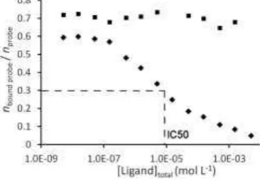
added concentration (not the free concentration) of either the target analyte or the competitor. This is the principle of the competitive binding assay, or molecular imprint sorbent assay (MIA) first demonstrated for MIPs in a seminal Nature pa-per by Mosbach et al. in 1993 [25]. For best results, nprobe is chosen to be as low as

possible (subject to the need for the proportion free in solution to be measured ac-curately by scintillation counting), the solvent and amount of imprinted material are then chosen such that when there is no additional target analyte or competitor, nbound probe / nprobe is in the range 0.5 to 0.8. Results for caffeine and theophylline

binding to a caffeine-imprinted polymer are shown in figure 12.

Fig. 12. Data for a MIA measuring the displacement of 14C-caffeine probe from a caffeine-imprinted MIP by non-labelled caffeine (diamonds) and by theophylline (squares) [23]. Assays performed in 1 mL volume of heptane/THF (3:1 v/v) using 8 mg of MIP and varying amounts of unlabelled caffeine / theophylline.

The increased displacement of the probe from the MIP as the total concentra-tion of target analyte is increased may be understood in terms of the binding iso-therm for caffeine on this polymer as shown in figure 6. At very low concentra-tions, the distribution ratio B/F takes a relatively high value (e.g. 0.004 nmol mg-1 / 0.02 M = 0.2 mL mg-1, from which it may be calculated nbound / nanalyte ~ 0.6, in

agreement with figure 12). At high concentrations B/F takes a lower value, due to the curvature of the isotherm data (e.g. 30 nmol mg-1/ 5000 M = 0.006 mL mg-1, from which it may be calculated nbound / nanalyte ~ 0.04, also in agreement). At about

B/F = 0.05 mL mg-1, from which it may be calculated nbound / nanalyte ~ 0.3. The

in-termediate value where nbound probe / nprobe is exactly half the value it was in the

ab-sence of any non-labelled analyte, is known as the IC50. The relationship between the adsorption isotherm and the radioligand competition displacement curve is fur-ther discussed by Pap and Horvai [16].

Comparison of IC50 values for the target analyte and a particular competitor provides evidence for selectivity: if the sites which bind the probe are selective, then a competitor should be less effective at displacing the probe than the target analyte, and have a higher IC50. From figure 6 it may be seen that for this poly-mer, the IC50 for theophylline is in excess of 3mM and using equation 18 the MIA cross-reactivity is consequently ~ 0.3%. However, while the IC50 for the an-alyte can be related to the isotherm, as outlined above, there is no such simple re-lationship between the isotherm for the competitor and the IC50 value of the com-petitor, and the MIA cross-reactivity cannot readily be related to the selectivity of a batch binding experiment as described in equation 6.

M�A cross reactivity analyte

competitor (18)

3c. Zonal chromatography

In many works, imprinted materials have been characterized by packing them into chromatography columns and measuring the retention times (tR) of the analyte,

and of competitors, when these are injected into a mobile phase flowing through the column. If the analyte exhibits a longer tR than the competitor, this provides

evidence for selectivity. This approach has been particularly used to demonstrate the separation of chiral mixtures, where one of the two enantiomers has been used as the template compound to generate an imprinted chiral stationary phase [50].

In conventional zonal chromatography under ideal, linear conditions, the reten-tion time for an analyte should be related to its distribureten-tion ratio via equareten-tions 19-20:

analyte R analyte R analyte (19)

and

analyte

mobile phase (20)

where t0 is the void time (the retention time for a non-retained species), tR, analyte

is the corrected retention time (=tR - t0), k analyte is the capacity factor, Mstationary phase

vol-ume of mobile phase (in mL). In theory, then, measurement of tR enables

calcula-tion of D.

This simple model has been extended by various authors to consider the effects of the concentration of a modifier(/strong eluent) in the (weak) eluent on kanalyte,

and, hence, to propose the stoichiometry and affinity of the modifier-analyte, ana-lyte-binding site and modifier-binding site interactions [51-53].

If tR is measured for a competitor then

analyte competitor

analyte R, competitor

R analyte

R competitor (21)

In this way, selectivity factors are frequently calculated for the separation of peaks due to the imprinted, and non-imprinted enantiomers on an imprinted chiral stationary phase (Figure 13). However, this approach (like those in the previous paragraph) is based on the assumption that D is independent of the total amount of analyte injected, i.e. that the isotherm is linear, whereas in practice the isotherm is curved, so that D falls as the total amount of analyte increases (this can be seen from the chromatograms for increasing concentration of analyte in figure 14). Again, the highest values for will usually be calculated when the ratio nanalyte /

MMIP is as small as possible i.e. when the lowest detectable amounts of analyte and

competitor are injected onto the column (and when both the imprinted, and non-imprinted enantiomers will have longer retention times).

Fig. 13. Separation of enantiomers of ephedrine by zonal chromatography on an MIP stationary phase. (-)-ephedrine imprinted MAA-EDMA copolymer packed into 250 x 4.6 mm column. 200 g (+/-)-ephedrine injected, chromatogram recorded at 254 nm using mobile phase of 20% AcOH in DCM, at 1.0 mL min-1 _{and 30º C[54].}

Three measures of the quality of a chromatographic separation which are com-monly encountered are the plate number N (which describes the sharpness of a peak), the asymmetry As (which describes the tailing or fronting of a peak) and the

resolution Rs (which is a ratio of the separation of two peaks over their width). In

the ideal case, N and Rs are independent of the amount of analyte loaded, and As =

The extreme tailing of the peaks often observed for zonal chromatography of analytes on MIPs (in particular, for the imprinted molecule itself) is attributed to the inhomogeneity of the binding sites and to slow binding/unbinding kinetics (the shape of the peaks can usually be improved by increasing the temperature of the column, which makes the rates faster) [55]. In figure 14, one can imagine the peak for 10 g of analyte representing the binding to the strongest binding sites on the polymer: when 20 g are injected there is too much anayte for the strongest bind-ing sites, such that weaker sites are occupied too, givbind-ing a ‘front’ to the 10 g peak. Likewise, one can picture the peak for 40 g of analyte building on the front of the 20 g peak, that for 100 g of analyte building on the front of the 40 g peak etc., as the extra analyte may only be retained by occupying weaker and weaker sites.

Fig. 14. Typical effect of increasing the amount of analyte injected on an MIP stationary phase in HPLC. MIP column is the same as for figure 13, chromatograms recorded at 254 nm using mobile phase of 5% BuNH2 in DCM, at 1.0 mL min-1 and 30º C. Injections of increasing

amounts of (-)-ephedrine: 10 g (bottom), 20 g, 40 g, 100 g, 200 g (top). Peak at ~ 3 min is the void peak due to the solvent in which analyte is injected[54].

More sophisticated models of chromatographic behavior incorporating non-ideality and/or non-linearity begin with the general rate model, in which the mass balance for an analyte at distance z along the column and time t after injection is given by:

p

L (22)

where C is the analyte concentration in the mobile phase (c.f. F, mol L-1), u is the linear flow rate (cm s-1),  is the porosity as a fraction of the column volume, Cp is the analyte concentration in the pores (such that  × total volume × Cp = M ×

B) and DL is the dispersion coefficient (cm2s-1), which is due largely to axial

chromatography, to fit the peak shapes for (large volume and large concentration) injections of Fmoc-Trp enantiomers on an Fmoc-L-imprinted MIP, and derived kinetic parameters [56-60]. Horvai et al. have shown that if ideal behavior (ne-glecting kinetic effects) is assumed, points on the trailing edge of a peak such as that in figure 14 can be related to points on the isotherm [18,61] (the ‘elution by characteristic point’ method). Seebach and Seidel-Morgenstern used a similar rela-tionship between the retention times for the peak maxima at a series of injected concentrations and B/F to derive an isotherm for Z-L-Phe binding to a Z-L-Phe MIP [62]. Baggiani et al. used a model derived from equation 22 but assuming a Langmuir-type isotherm to fit the complete peak shape for injections of pyrime-thanil on pyrimepyrime-thanil-imprinted MIPs, deriving apparent site densities and affini-ty constants as well as kinetic parameters [63]. Lee et al. have modelled the effect of sample concentration and affinity constant on the plate number and peak asymmetry [64].

3d. Frontal chromatography

In simple (‘rectangular pulse’) frontal chromatography, instead of injecting a short pulse of analyte, the mobile phase is altered to contain a specific concentration of analyte, which is run continuously through the column [65-67]. Initially, as it first enters the column, the analyte binds to binding sites on the stationary phase, how-ever once the bound concentration of analyte reaches equilibrium with the concen-tration in the mobile phase over the whole of the column (as may be expressed via the distribution ratio for the analyte under those conditions) no more analyte can bind, and the analyte begins to elute from the column, the concentration in the elu-ent soon becoming the same as in the mobile phase which continues to be fed on to the column. The measured parameter is the breakthrough time, tbreakthrough (or,

frequently, the breakthrough volume, Vr in mL, which is just tbreakthrough × the

vol-umetric flow rate (f, L min-1)), which is the interval from the point at which the mobile phase is changed, to the time when the analyte appears in the eluent.

The amount of analyte bound to the stationary phase is given by:

bound breakthrough (23)

where t0 is the void time as before (and will correspond to tbreakthrough if none of

the analyte at all was to bind to the stationary phase), and [A] is the concentration (mol L-1) of analyte added to the mobile phase. The distribution ratio (equation 3) is given by:

breakthrough

and hence the binding isotherm can be derived. Data obtained in this way can readily be fitted to a model assuming all binding sites are equivalent (i.e. a Lang-muir model). If this is the case, the total number of binding sites ntotal is given by

ntotal = nempty + nbound and (from equation 2)

d empty

bound

total

bound (25)

substituting F=[A] and for nbound as in equation 23 gives

d _breakthroughtotal (26)

Thus, a series of experiments are performed applying different concentrations of analyte in the mobile phase. tbreakthrough is measured, then the column

regenerat-ed to remove all bound analyte and the experiment repeatregenerat-ed using a different con-centration. A plot of 1/([A]×f×( tbreakthrough - t0)) against 1/[A] should give a straight

line with y-intercept 1/ ntotal and x-intercept -1/Kd.

Mosbach et al. were first to apply this approach to MIPs, deriving apparent ntotal

values in the range 18-28 mol g-1 of polymer, Kds in the range 1.6 to 8.1 mM, and

showing that MIPs had lower Kd values (indicating stronger binding) for their

template than its optical antipode, and lower Kds than the corresponding NIPs, as

expected [68,69]. Andersson et al. applied frontal chromatography to a model sys-tem of pyridines and bipyridines binding to 4,4’-bipyridyl-imprinted MAA-co-EDMA in order to demonstrate the increased strength of binding when more than one analyte-monomer interaction is present within the imprinted site [70]. The ap-proach has also been used extensively by Baggiani et al.[71,72] and others [73,74]. In one intriguing study, Baggiani et al. compared the rebinding of 2,4,5-trichlorophenoxyacetic acid (2,4,5-T) to a conventional 2,4,5-T-imprinted 4-vinylpyridine-co-EDMA polymer and a polymer which, additionally, incorporated a covalently bound template analogue, and showed that the latter polymer had a lower binding capacity (lower ntotal) but lower Kd (i.e., the covalently incorporated

template analogue appeared to increase the strength of template re-binding)[3]. A variant of frontal chromatography is staircase frontal chromatography, in which, once the detector signal has stabilized showing that the analyte is present in the eluent at the same concentration as in the injected mobile phase, the mobile phase is altered to contain a higher concentration of the analyte, and the process repeated giving a chromatogram with the appearance of a staircase, indicating a series of concentration steps. This approach was first applied to MIPs by Gui-ochon et al. [29]. On proceeding from step i to step i+1, the additional amount of analyte bound to the stationary phase can be calculated as :

from which the isotherm can be derived in shorter time than would be required by the rectangular pulse method (where the column must be regenerated between each change in concentration). Figure 15 shows typical data.

Fig. 15. Partial frontal chromatogram of caffeic acid on caffeic acid-imprinted MAA-co-EDMA monolith in a 200 x 4.6 mm column with THF mobile phase at 25 ºC and 0.5 mL min-1, moni-tored at 280 nm. Arrows mark introduction of sample solutions having the concentration indicat-ed. Reproduced with permission from [28].

The shape of the ‘front’ or breakthrough curve can also give information about the shape of the isotherm, as well as the kinetics of analyte binding to the station-ary phase. For example, figure 16 shows a typical breakthrough curve obtained by Guiochon et al. tbreakthrough is the time corresponding to half-height of the front, i.e.

the centre of mass of the concentration step, in this case 6.75 min. A classical transport model was applied to model the breakthrough curve, involving numeri-cal solutions of an equation derived from equation 22. The modelled curves re-quire as an input a relationship between B and F for any particular F at equilibri-um (i.e. a theoretical isotherm, see section 2), and an estimated value for the mass transfer rate coefficient kf (in min-1), which is related to, though not identical to,

the forwards rate constant k1 in equations 7 and 8, and defined as:

Fig. 16. Experimental breakthrough curve (symbols) and fitted curves (lines) for L-Phe-An ap-plied to a L-Phe-An imprinted MAA-co-EDMA polymer, packed into a 100 x 4.6 mm column. Mobile phase of MeCN-0.05 M potassium phosphate (7:3 v/v) at 1.0 mL min-1 and 40°C, moni-tored at 260 nm. The concentration step shown is from Cn=0.01 to Cn+1=0.02 g/l. Calculated

breakthrough curves for kf=10 min−1, kf=110 min−1 and for the rate coefficient which fits best the

experimental data, kf=40 min−1 (the larger kf, the steeper the curve). Solid lines: Bi-Langmuir

model. Dashed lines: Freundlich model. Reproduced with permission from [29].

For the concentration step shown in figure 16, the classical transport model provides the best fit to the data when the isotherm is considered to be of the bis-Langmuir form and kf is given the value 40 min-1. For a sequence of concentration

steps, kf was found to increase with an increase in [A], to increase with

tempera-ture, and to be lower for the imprinted enantiomer than its optical antipode (par-ticularly at lower concentrations). The latter effect may be rationalized by the strongest, most selective binding sites being also the less accessible, hence slower binding ones [29]. The values of kf found are low in comparison with other types

of stationary phase, supporting the thesis that slow mass transfer contributes to the poor peak shapes seen in zonal chromatography, as well as binding site heteroge-neity.

Staircase frontal chromatography was used further, in combination with models of non-ideal, non-linear chromatographic behavior, in a series of works by Gui-ochon et al. to show the effects of heat-treating the MIP [75,76], the effects of the pH [77] and temperature [60] of the mobile phase, the effects of different organic mobile phases [78], of organic modifiers added to an acetonitrile mobile phase [79,80], and of water in an organic-aqueous cosolvent mobile phase [58], to com-pare particulate and monolithic MIP stationary phases [81], to comcom-pare the reten-tion of template analogues [82] and to deconvolute the effects of different kinetic processes in the lumped mass transfer rate coefficient kf: it was shown that in

3e. Calorimetry

When the target analyte (or a competitor) binds to an imprinted binding site, there is expected to be a change in enthalpy H. If the binding process is thermodynami-cally favorable then the change in Gibbs free energy, G for the process must be negative, where G is related to the changes in enthalpy and entropy, S:

(29)

Hence a spontaneous (exergonic) process can be driven by a negative H (exo-thermic) or by a positive S (increase in entropy). Bond formation is usually exo-thermic.

Fig. 17. (A) Experimental titration curves for the titration of BocLPheAn imprinted and -extracted microgel A at 25ºC (I) and the corresponding control dilution experiment (II). Measured heat power vs. time. A suspension of microgel in methanol/water (50:50 v/v) was titrated into Boc-L-Phe-An dissolved in the same solvent. (B) Observed titration heat Qstep versus

molar ratio microgel to template (the first value was excluded from analysis). Reproduced with permission from [90].

The sample in the cell might be the imprinted material, with the target analyte added from the syringe, but in the experiment shown in Figure 17 the set-up was with the target analyte (Boc-Phe-An) in the cell and a suspension of imprinted na-noparticles in the syringe [90]. When the adsorption isotherm has been obtained independently, it may be possible to know exactly how much analyte binds to the imprinted polymer in each step (nbound after step – nbound before step), in which case:

bound after step bound before step (30)

If the binding isotherm is not known, the data can be converted to display Q cu-mulative against [titrant]total and fitted with a function assuming a single class of

bound cumulative (31)

total bound analyte bound (32)

where M and V have their usual meaning. This yields nbound as the root of a

quadratic, and the function can be fit to yield H, ntotal and Ka (in the case of

We-ber et al. [90], ntotal was estimated independently).

In these or equivalent ways, quite varying values of H have been obtained: +8 kJmol-1 for 2,4-D binding to a imprinted VPy/EDMA polymer in aqueous buffer [84], +6.6 kJmol-1 for phenylmannopyranoside binding to a vinylphenylboronic acid/EDMA polymer in acetonitrile [88], -21 kJmol-1 for Boc-L-Phe-An binding to the polymer shown in figure 17 [90], -8 kJ kJmol-1 for riboflavin binding to a 2,6-bis(acylamido)pyridine polymer in water/ethanol/formic acid (90.6:4.7:4.7 v/v/v).

In some cases, the further extension has been made that, if the conditions can be approximated to standard conditions,

(29)

and since

ln (30)

the entropy change on binding, S may also be estimated. There seem to be ra-ther too many assumptions underlying quantitative estimates like this: however it may certainly be said that if the process is observed to be endothermic, as in Chen et al.s study of 2,4-D binding to a imprinted VPy/EDMA polymer in aqueous buffer [84], then the binding must be driven instead by an increase in entropy. This makes sense in the case of binding in water, where hydrophobic interactions are well-known to be entropically driven.

3f. Other methods

Since the application envisaged for many MIPs is in solid-phase extrac-tion/sample clean-up of a dilute analyte in a complex matrix prior to quantitative analysis by HPLC, LC-MS or GC, Martin-Esteban et al. have attempted to derive isotherms for analytes binding to MIPs under SPE-type conditions [35,36,93]. In an experiment which is similar to a batch-binding experiment, analyte in binding solvent (1 mL, 0.05 – 500 mg L-1

) was loaded onto pre-conditioned MIP (100 mg) packed into a SPE cartridge. Some, but not all, the analyte bound under these con-ditions. A washing solvent was applied, followed by the elution solvent (3-8 mL). The eluted fraction was concentrated, and analysed by HPLC to determine nbound.

Data were then fitted using Langnuir-Freundlich isotherms. Although the ap-proach was certainly useful in characterizing MIPs for SPE, the validity of the iso-therm fits is questionable because binding did not necessarily occur under equilib-rium conditions, and there is no way of assessing the effect of kinetic limitations.

Spectroscopic interrogation of an MIP, in its clean state and after binding of analyte, forms the basis of many proposed applications of MIPs in chemical sens-ing. However, such an approach can also provide useful information about the na-ture of analyte-binding site interactions, including some indication of their strength. Hsu et al. used infrared (IR) spectroscopy to monitor the binding of thy-mine to thythy-mine-imprinted diacryloyl-2,6-diaminopyridine-co-tripropyleneglcol diacrylate polymer films in chloroform [94]. Distinctive absorbances were ob-served due to the bound and non-bound thymine: by assuming the measured ab-sorbances to be proportional to B and to F, apparent binding constants Ka could be

calculated. Resmini et al. used a similar approach based on the quenching of the visible absorbance (435 nm) of a phosphate template when it rebinds to an argi-nine-containing MIP in DMSO, to calculate the binding site population (assuming a stoichiometric rebinding) [95]. Haupt et al. used the Raman signal produced when propranolol was added to a propranolol-imprinted MIP and a NIP in MeCN to plot a form of isotherm and calculate apparent binding constants Ka (their

ap-proach assumes the free propranolol concentration is identical to the added con-centration) [96]. In each of these examples, the sensor response (change in absorb-ance of the polymer) is assumed to be proportional to B (or nbound). This

assumption was tested for two MIP systems by Ng and Narayanaswamy [97]. Cu2+

binding to copper-imprinted 4-vinylpyridine-co-hydroxyethylmethacrylate-co- EDMA polymer particles in water was measured both by batch binding (superna-tant added to eriochrome cyanine R and absorbance recorded at 568 nm) and by reflectance measurements at 750 nm on a layer of particles deposited on the tip of a fibre-optic bundle. N-phenyl-1-naphthylamine (NPN) binding to NPN-imprinted 2,4-diisocyanate cross-linked -cyclodextrin particles in methanol was measured by batch binding (direct measurement of supernatant absorbance at 340 nm) and fluorescence measurements ( ex = 365 nm, em = 495 nm) on particles trapped in a

fluorescence flow cell. The authors suggest a good correlation in each case, alt-hough a simple comparison of signal and B for differing F is not presented: more studies of this kind are needed in order to correlate sensor signals with binding isotherms.

Apparent isotherms can be recorded, and apparent affinity constants calculated, using other sensor techniques such as surface plasmon resonance [98] and quartz crystal microbalance [99,100]. Such analyses again rely on the assumption that the sensor response is proportional to B (or nbound).

binding of fluorescein-labelled cytochrome-C from aqueous buffer [101]. Recent work by Reddy et al. [102], yielded similar data for the binding of bovine hemo-globin (immobilized on an AFM tip) to protein-imprinted hydrogel particles.

In parallel with experimental studies, the interactions of analytes with MIPs have been modelled in silico [103]. Although there are less examples of computa-tional studies on MIPs than on the pre-polymerization mixture (reflecting the greater complexity of the polymerized material), this is a field of increasing activi-ty.

4. Parameters influencing rebinding

4a. Polymer design

MIP design cannot be dealt with in this chapter, but it should be emphasized that the binding properties of a MIP (and NIP) are inextricable from its composition and method of preparation. The major factors influencing the binding properties of the resulting polymer include the type of functional monomer and mono-mer:template ratio [1,9,104-106] and the porogenic solvent [105,107].

4b. Rebinding solvent (organic solvents)

made with MeCN as porogen and exhibited higher affinity and selectivity for the template in MeCN than in DCM, chloroform, or THF. The isotherm in MeCN was well-fitted to a tri-Langmuir model, but in the other solvents a bi-Langmuir model fitted best suggesting that the strongest adsorbing sites were absent [78]. The in-fluence of solvent dielectric constant and Snyder polarity index on rebinding of bupivacaine to a bupivacaine-imprinted MAA-co-EDMA in single-point experi-ments has been studied by Rosengren et al. [109].

Commonly a polar organic modifier is added to the organic solvent in which analyte binding to a MIP is being studied – the modifier serves to reduce the strength of binding. This is often desirable so as to promote selective binding, ra-ther than non-selective i.e. the modifier is thought to reduce binding to the weak, non-selective hydrogen bonding sites of the polymer more than it reduces binding to the strong, selective sites [9]. In MIA binding assays, in SPE, and in the use of MIPs as stationary phases in chromatography, the effect of increasing amounts of modifier on binding to the MIP and NIP is often compared, to find the modifier concentration at which the IF is maximized. The influence of type and concentra-tion of modifiers on the binding of Fmoc-L-Trp to Fmoc-L-Trp-imprinted 4-VPy-co-EDMA particles was also studied in detail by Guiochon et al. using staircase frontal analysis. Isotherms were obtained and fitted to tri- or tetra-Langmuir mod-els. Modifiers were found to reduce the density, Bmax of the strongest binding sites

more than the Ka, but reduce the Ka of the weak binding sites more than their Bmax

[79,80].

4c. Rebinding pH and cosolvent (aqueous)

MIPs dependent on weak hydrogen bonds between the template and binding site do certainly work best in organic solvents, and furthermore the sugar-imprinted polymers studied by Wulff in the 1970s and 1980s (based on the cova-lent interactions between sugars and boronic acids) had a similar preference. This led to a prejudice among the wider scientific community that MIPs could not work in aqueous solvents. Nowadays there are numerous examples of MIPs both made in, and applied in, aqueous buffers or aqueous / organic cosolvent mixtures. MAA- or 4-VPy-based polymers can show good binding and selectivity in aque-ous buffers if the analyte-polymer interaction is strong [110,111].

functional groups of the MIP are ionizable. Sellergren and Shea proposed a model for the influence of pH on retention and separation of the enantiomers of Phe-An on a Phe-L-An-imprinted MAA-co-EDMA polymer in zonal chromatography [113]. At pH 4 and below, both the analyte and the carboxylate groups of the MIP are protonated, the cationic analyte interacts only weakly with the neutral poly-mer. At pH 8 and above, both the analyte and the carboxylate groups of the MIP are deprotonated, the neutral analyte however interacts only weakly with the ani-onic polymer. In the intervening region, there is some overlap between the car-boxylate groups being deprotonated and anionic and the analyte protonated and cationic – so binding is strongest. However, selectivity peaks at about pH6, which was proposed to correlate with the carboxylate functions of the strongest, most se-lective sites having a lower average pKa than the weaker, non-selective sites.

Guiochon et al. have also studied the influence of the fraction and pH of aque-ous cosolvent in an acetonitrile mobile phase on the isotherms for Phe-An [77] and Fmoc-Trp [58] enantiomers on their respective MIPs, obtained via staircase frontal analysis. In the former case, the isotherms supported the conclusions of Sellergren and Shea, with the number of weak binding sites increasing faster with pH than the number of strong binding sites. For Fmoc-Trp, the highest number of binding sites was calculated at pH3.8, where both the analyte and polymer (4-VPy based) are neutral: this corresponded to zonal chromatography where the highest retention was at this pH. Selective binding in this case appears to be driven more by hydrophobic interactions and hydrogen bonds, than by ion-pair formation.

4d. Temperature

The first detailed study of the effect of temperature on MIP binding properties was reported by Sellergren and Shea [55]. The binding of the enantiomers of Phe-An to an L-Phe-An-imprinted MAA-co-EDMA polymer was studied in zonal chroma-tography using an MeCN-aqueous buffer mobile phase and an MeCN-AcOH mo-bile phase at temperatures between 20 and 80 ºC. For the aqueous momo-bile phase, increasing temperature lead to a partial improvement in the peak shape (suggest-ing an acceleration of the kinetics), a decrease in the retention of both enantiomers (suggesting binding is an exothermic, enthalpy-driven process) and a decrease in separation (suggesting binding of the imprinted enantiomer is more exothermic than that of its optical antipode). For the organic mobile phase a partial improve-ment in the peak shape was again observed, but there was an increase in the reten-tion of both enantiomers (suggesting binding is an endothermic, entropy-driven process) and an increase in separation.

Hsu et al. also studied the effect of temperature on the Ka values obtained for

in-crease in temperature, and an exothermic H and corresponding S were calculat-ed.

Guiochon et al. also studied the influence of the temperature on the isotherms for Fmoc-Trp enantiomers on the Fmoc-L-Trp-imprinted MIP, via staircase frontal analysis with an MeCN-AcOH (99:1 v/v) mobile phase [56,57,60]. H, S and kinetic parameters were calculated for the different classes of site that appeared to contribute to the isotherms fitted with bi- and tri-Langmuir models. Whilst it was concluded that binding overall was enthalpy-driven, the dominant driving force for transfer of the imprinted enantiomer to the strongest, most selective sites was proposed to be entropic.

5. Binding site affinity distributions

The number of binding sites and their binding affinities are parameters in the Langmuir, bi-, tri-and multi-Langmuir isotherms: hence when an isotherm is fitted using these models, a simplistic picture of the classes of sites (each class having a unique Ka and Bmax) is immediately available. In reality, however, as explained in

the introduction, there will not be distinct classes of binding sites but rather a con-tinuum, from strong and selective sites present in small numbers to weaker and less selective sites present at far greater densities. Both the Freundlich and Lang-muir-Freundlich isotherms allow for such a distribution of sites, and the number of sites Bi with a particular affinity constant Kai can be calculated from the isotherm

fitting and displayed as an affinity distribution (figure 18). These models are re-strictive however, in that the shape of the distribution is fixed (for the Freundlich isotherm, it is an exponentially decaying distribution starting with an infinite number of binding sites with Ka = 0, for Langmuir-Freundlich, it is a gaussian

dis-tribution). An alternative approach involves converting the isotherm data directly to an affinity distribution without applying any fixed isotherm model: such an ap-proach is valuable but depends on data of extremely high quality.