M a th e m a tic a l a n d S ta tis tic a l
M o d e llin g fo r A ir Q u a lity
M a n a g e m e n t
J u n Bai
U
l
,
brary
d
A th e sis su b m itte d to th e
A u stra lia n N a tio n a l U n iv ersity
for th e d egree o f D o cto r o f P h ilo so p h y
P R E F A C E
T h e following are publications prepared during th e period of this course and under taken as jo in t research with Anthony J. Jakem an, Michael McAleer, John A. Taylor of ANU, and G erald Miles of the N ational C apital Planning Authority.
(1) B a i, J . a n d T a y lo r, J .A . (1986), E stim ation of the param eters and upper percentiles of statistical distributions applicable to air quality d ata, p art I: T he gam m a distribution. CRES Working Paper, No 1986/39, A ustralian N ational University, pp. 131.
(2) T a y lo r, J .A ., J a k e m a n , A .J . a n d B a i, J.(1986), A Monte Carlo study of estim ation of the upper percentiles of the three-param eter gam m a distribution using m ethods of moments and m axim um likeli hood. CRES Working P ap er, No 1986/34, A ustralian N ational Uni versity, pp. 16.
(3) J a k e m a n A .J ., B a i, J . a n d T a y lo r, J .A . (1988), On th e variabil ity of the wind speed exponent in urban air pollution models. A tm o spheric Environm ent, 22 (9), 2013-2019.
(4) B a i, J . , J a k e m a n A .J . a n d T a y lo r, J .A . (1988), Statistical dis tribution modelling: Function, m ethods and application to air quality m anagem ent. M athem atics and Com puters in Sim ulation, 30, 3-9.
(5) T a y lo r, J .A ., J a k e m a n , A .J . a n d B a i, J . (1988), Modelling for air quality m anagem ent. 12th World IMACS Congress on Scientific C om putation, 18-22.
(6) M ile s, G .H ., J a k e m a n , A .J . a n d B a i, J . (1989), A m ethod for predicting the future extrem es of urban air pollution from vehicle emis sion, meteorology and historical concentrations. Proceedings of the Sim ulation Society of A ustralia Conference, 418-423.
(8)
(9)
(10)
(11)
(12)
(13)
Bai, J., Jakeman, A .J. and M cAleer, M.
(1989), The estimating
the percentiles of some misspecified non-nested distributions. Working
Papers in Economics and Econometrics No. 193, Australia National
University, December 1989. (also submitted to Communications in
Statistics).
Bai, J., Jakeman A .J. and Taylor, J.A .
(1990), Percentile es
timation of the three-parameter gamma and lognormal distribution:
methods of moments versus maximum likelihood. Mathematics and
Computers in Simulation, 32, 164-169.
Bai, J., Jakeman, A .J. and M cAleer, M.
(1990), The effects of
misspecification in estimating the percentiles of some two- and three-
parameter distributions. Mathematics and Computers in Simulation,
32, 194-199.
Bai, J., Jakeman, A .J. and M cAleer, M.
(1990), Discrimination
between nested two- and three-parameter distributions: An applica
tion to models of air pollution. Working Paper in Economics and
Econometrics No. 197, Australian National University, March 1990,
pp. 23. (also submitted to Technometrics)
Bai, J., Jakeman, A .J. and M cAleer M.
(1990), Discrimination
procedure for fitting nested and non-nested distributions to environ
mental quality data. Working Papers in Economics and Econometrics
No. 200, Australian National University, March 1990, pp. 58. (also
submitted to Environmentrics)
Jakeman, A .J., Bai, J. and M iles, G.H.
(1990), Prediction of non
stationary extremes of one-hour average urban CO concentrations,
(submitted to Atmospheric Environment)
The text of these papers has been closely followed in Chapters 3 to 12 of this thesis.
Unless otherwise acknowledged in the text, the remainder of this thesis represents the
original research of the author.
J u n B a i
A C K N O W L E D G E M E N T S
I would like to thank my supervisory panel of Anthony J. Jakeman, Michael McAleer,
Michael Hutchinson and Rodney Simpson for their advice and general guidance. I am
particularly indebted to Tony Jakeman and Michael McAleer for their direction, en
couragement, and kindly giving of their time to the development of the study and
formation of this thesis. Special thanks also go to John Taylor for his kindly advice on
technical issues.
I am also grateful to the following for their assistance: Gerald Miles of the National
Capital Planning Authority, and G. Moynihan of the Canberra branch of the National
Climate Centre, Australian Bureau of Meteorology. They provided the air quality data
and the meteorological data recorded in Canberra, respectively.
I have received welcome assistance from Tony Bayes in the management and organi
sation of the data sets used in the thesis, from Mark Greenaway of CRES for equipment
operation and production of graphics, and from Kathy Handle of the Computer Services
Center for advice on available computer software and techniques.
Many thanks to Henry Nix, Director of CRES, for his profound concern, and en
couragement throughout my candidature. Also thanks to my friends and colleagues
at CRES who provided an interesting and stimulating environment within which this
research was undertaken.
I am very grateful to Ian Taylor and Wendy Chen for careful proof-reading of the
final draft of this thesis.
Thanks go to my family and friends, especially to Alejandra Benedictos for her
support during my period of intensive research.
A B S T R A C T
Air quality m anagement requires th e developm ent of relationships between th e fre quency distribution of ambient pollutant concentrations at sites of concern and emis sions, meteorological and other forcing variables. In this thesis, m athem atical models are devised to achieve a range of goals w ithin this basic objective. In A ustralia, much recent effort has been devoted to both statistical and hybrid determ inistic-statistical d istribution modelling approaches which have extensive potential but previously have been given only limited attention in th e literature.
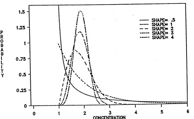
These are the approaches investigated in this thesis, although it should be em pha sised th a t th e so-called statistical models should more appropriately be labelled fre quency or probability distribution models as they are param etric forms of probability density functions. There are six param eterisations used in the thesis and these are th e two- and three-param eter versions of the gam m a, Weibull and lognormal distributions.
Basically, each of the two approaches treated has its own assum ptions and the choice of approach depends on the goal, th e validity of the assum ptions and th e d a ta available. Each approach must also invoke a m ethodological infrastructure. Generally, th is involves the use of adequate techniques for identification of an appropriate p a ra m etric form to represent a given pollutant d a ta set and for estim ation of th e associated p aram etric values and the ensuing errors.
as methods of moments can suffice if the objective is merely to summarise the data
and/or to allow high variance estimates. It shows how to construct error models that
allow the calculation of the minimum errors in percentiles to be expected when fitting
samples from different probability distributions. The thesis also evaluates errors of mis-
specification which arise when the wrong parametric form of distribution is selected.
All of these tools are then combined to illustrate the practical use of a comprehensive
procedure to identify a suitable parametric form which represents a given pollutant
over the years at single and multiple sites. It should also be mentioned that much of
the new technology developed for the statistical aspects of the thesis can also be used
for application of extreme value theory in statistics since the same identification and
estimation tools are required.
C o n te n ts
I
IN T R O D U C T IO N
1
1 A S y s te m s A pproach to A ir Q u a lity M a n a g e m e n t 2
1.1 Introduction...
2
1.2 Air Quality M anagem ent...
5
1.3 Air Quality Standards ...
5
1.4 Thesis O utline...
7
2 R e v ie w o f A ir Q u a lity M o d e llin g 12
2.1 Introduction...
12
2.2 Deterministic Models for Air Pollution Concentrations ...
13
2.3 Deterministic Models for Air Pollution Concentrations ...
14
2.3.1
Gaussian Plume M o d e ls ...
14
2.3.2
K-Theory M o d els...
16
2.3.3
Box M o d e ls ...
17
2.3.4
Performance and Validation of Deterministic Models ...
24
2.4 Statistical M o d ellin g ...
27
2.4.1
Probability Distribution M o d e llin g ...
28
2.4.2
Stochastic M o d ellin g ...
30
II ESTIMATION
36
3 A N e w A p p roach to M a x im u m L ik e lih o o d E s tim a tio n o f th e T h r ee
-P a r a m e te r D is tr ib u tio n s 37
3.1 Introduction...
37
3.2 A General Approach to Maximum Likelihood Estimation of the Three
Parameter Gamma and Weibull D is trib u tio n s ...
39
3.3 A New Approach to Maximum Likelihood E stim a tio n ...
41
3.4 Improved General Approaches for the Gamma D istrib u tio n ...
42
3.5 Simulation E x p e rim e n ts...
43
3.6 Fitting Real D a t a ...
46
3.7 Discussion of the Maximum Product of Spacings (MPS) Estimation
Method ...
47
3.7.1
MPS Estimation of the Gamma D istrib u tio n ...
48
3.7.2
Comparison of the ML and MPS Methods for the Weibull Dis
tribution ...
49
3.8 Concluding R e m a rk s ...
50
4 P e r c e n tile E stim a tio n : th e M e th o d o f M o m e n ts v ersu s M a x im u m L ik elih o o d 60
4.1 Introduction...
60
4.2 General Properties of the Methods of Moments and Maximum Likeli
hood related to Air Quality Application ...
61
4.3 Estimation by the Method of M o m e n ts...
64
4.3.1
The Characteristic Function and M o m e n ts...
64
4.3.2
The Moments Estimators for Two- and Three-parameter Gamma,Weibull
and Lognormal D istributions...
67
4.5 Monte Carlo E x p e rim e n ts ...
72
4.6 Monte Carlo R e s u l ts ...
73
4.6.1
Estimation for the Three-parameter Gamma Distribution . . . . 73
4.6.2
Estimation for the Three-parameter Weibull Distribution . . . . 75
4.6.3
Estimation for the Three-parameter Lognormal Distribution . .
77
4.6.4
Estimation for the Two-parameter Gamma, Weibull and Lognor
mal D istributions...
79
4.7 Concluding R e m a rk s ...
80
5 E m p ir ic a l M o d e ls o f F ittin g E rrors 98
5.1
Introduction...
98
5.2 Literature Review...
99
5.3 Empirical Model-building and the Similarity to Time Series Analysis .
99
5.4 The Response F unction... 100
5.4.1
Series Approximation...101
5.4.2
Deterministic A p p ro x im atio n ... 102
5.5 Empirical Model-building in Predicting RRMSE for Air Quality Man
agement ... 103
5.5.1
Hypothetical Response Function of R R M S E ...104
5.5.2
Transformation, Estimation and Identification...106
5.5.3
Simulation and Experimental D e s ig n ... 109
5.5.4
The Experimental R e su lt... I l l
5.6 Concluding R e m a rk s ... 114
III
D IS C R IM IN A T IO N A N D M IS S P E C IF IC A T IO N
127
-tio n s 128
6.1 Introduction...
. 128
6.2 The D istributions...
. 129
6.3 Discrimination C rite ria ...
. 131
6.4 Loss Functions ...
. 133
6.5 Simulation Procedure...134
6.6 Monte Carlo R e s u l ts ...
. 135
6.7 Application to Models of Air P o llu tio n ...
. 138
6.8 Concluding R e m a rk s ...141
7 T h e E ffects o f M issp e c ific a tio n in E s tim a tin g th e P e r c e n tile s o f Sem e T w o - and T h r e e -P a r a m e te r D is tr ib u tio n s 150
7.1 Introduction... 150
7.2 Distribution Functions and Statistical C r ite r ia ...
. 151
7.3 Monte Carlo E x p e rim e n ts...
. 153
7.4 Monte Carlo R e s u l ts ...
. 154
7.5 Concluding R e m a rk s ... 159
8 D isc r im in a tio n P r o c e d u r e s for F it t in g N e s t e d and N o n -N e s te d D is tr ib u tio n s 164
8.1 Introduction...164
8.2 Available P ro ced u res...166
8.3 Practical P ro b le m s ...
. 167
8.4 Discrimination Criteria and Asymptotic T e s t s ... 171
8.5 A Generalized Information Criterion (G IC )... 173
8.6 Distribution Functions and Statistical C r ite r ia ... 175
8.8 Discrimination Between Two Non-Nested Distributions
178
8.9 Discrimination Among Three Non-Nested D istributions... 185
8.10 Discrimination Among Five Non-Nested D istributions... 190
8.11 Discrimination Among Six Nested and Non-Nested Distributions . . . . 195
8.12 Concluding R e m a rk s ...200
9 E s tim a tin g th e P e r c e n tile s o f S o m e M issp e c ifie d N o n -n e s te d D is tr i b u tio n s 220
9.1
Introduction... 220
9.2 Distribution Functions and Performance C riteria...221
9.3 Monte Carlo E x p e rim e n ts... 223
9.4 Monte Carlo R e s u l ts ...224
9.4.1
Gamma Distribution is T r u e ... 224
9.4.2
Weibull Distribution is T r u e ...225
9.4.3
Lognormal Distribution is T r u e ...226
9.5 Concluding R e m a rk s ... 227
IV
A P P L IC A T IO N S TO A IR Q U A L IT Y M A N A G E M E N T
2 3 2
10 E stim a tio n and D is c r im in a tio n o f A lte r n a tiv e A ir P o llu tio n M o d e ls 23310.1 Introduction...233
10.2 Considerations for a Comprehensive Model Selection Procedure . . . . 236
10.3 Evaluating Misspecification E rro rs... 238
10.4 Fitting Real D a t a ...243
10.4.1 Detailed CO Results for the Museum Site ...243
10.4.3 Summary of Air Pollutant Distributions for Multiple Sites . . . 248
10.5 A Brief Discussion of the Results for Pollutants NO, NO
2, NOx and SO
2250
10.6 Concluding R e m a rk s ... 252
11 P r e d ic tio n o f N o n -sta tio n a r y S ea so n a l E x tr e m e s o f O n e-h o u r A v e r a g e U r b a n CO C o n cen tra tio n s 265
11.1 Introduction... 265
11.2 The Hybrid Approach ... 268
11.3 The Deterministic M odel...270
11.4 Parametric Form of Annual and Seasonal Distributions of Historical
C o n cen tratio n s... 275
11.5 A Hybrid Method and P re d ic tio n ... 277
11.6 Concluding R e m a rk s... 279
12 On th e V a ria b ility o f th e W in d S p ee d E x p o n e n t in U rb a n A ir P o llu tio n M o d e ls 285
12.1 Introduction... 285
12.2 The Data Set and Airshed C h a ra c te ristic s...286
12.3 Method and Results ... 287
12.4 Hybrid Modelling A p p ro a c h ...289
12.5 Use of Filtering and Smoothing Algorithm s... 290
12.6 Concluding R e m a rk s... 291
Appendix I ... 301
Appendix I I ... 314
P a r t I
C h a p te r 1
A S y s te m s A p p r o a c h to A ir
Q u a lity M a n a g e m e n t
1.1
I n tr o d u c tio n
T he atm osphere is an im p o rtan t shared resource whose quality needs protection. The deterioration of atm ospheric environm ental quality, related to changes in th e chemical, physical and biological n atu re of air brought about by industrial, agricultural and social activities, has becom e a th re a t to m any plant and anim al com m unities, and to th e hum an race. A system s approach to atm ospheric environm ent quality control is urgently required to provide an effective m eans of preserving for future generations some sem blance of th e biological order of th e world and to im prove th e deteriorating stan d ard of urban public health (M etcalf and P itts, 1972).
have becom e of m ore concern in recent years, are discussed.
A ppendix 1 also introduces th e im p o rtan t concepts which underlie any study of air quality. These concepts include definitions for the term s atm osphere, clean air and global background concentrations. In order to b e tte r un d erstan d air quality im pact as sessm ent, m ost air pollutants and th eir characteristics are sum m arised in the appendix, and some of th em will be chosen for m odelling in this thesis.
In recent decades, th ere have been great im provem ents in control technology, in u n d erstanding of atm ospheric processes and interactions am ong air-borne pollutants. T here have also been accom panying developm ents in adm inistrative and legislative in stru m en ts for regulation and ab atem en t of those pollutants. To develop m anagem ent of our atm ospheric resources fu rth er, m ore scientific inform ation is needed. For exam ple, de Nevers et al. (1977) have argued th a t a com plete and closed inform ation cycle m ight be required. T he inform ation would include emission d ata, air quality m onitoring and air quality m odelling results. If such associated analytical tools are widely available, th eir use m ay strongly influence decisions on any proposed or existing projects. Un fortunately, th ere is considerable uncertainty at present about all three factors in this inform ation cycle leading to m odel results of lim ited accuracy and validity. Therefore, each of th e factors m ust be im proved in order to develop a predictive scheme which can be used w ith confidence.
m odel o u tp u t.
A tm ospheric system s are, in th e term inology of Young (1978), ‘badly defined’ in th a t th e relationships th a t describe th eir behaviour are complex and not easily am enable to exploration through planned experim entation. T heoretically in such system s both causal and non-causal relations exist. For exam ple, m any determ inistic models a tte m p t to present an ideal p a tte rn of th e causal linkage am ong dependent and independent variables, such as in th e basic equations of m olecular diffusion. However, inherent in these system s are statistical features (e.g. Pasquill and Sm ith, 1983). A tm ospheric behaviour is essentially th e consequence of an hybrid determ inistic-statistical system . Therefore theory and techniques for bo th determ inistic and statistical m odelling ap proaches are required. It would be useful to develop a specific system m ethodology which can be applied to such a hybrid system .
T he aim of this thesis is to develop tools for the construction of sim ple bu t effective models to predict am bient pollutants which reduce the difficulties arising from lim ited meteorological inform ation, sparse pollu tan t m onitoring d a ta and th e stochastic n atu re of tu rb u len t diffusion processes. T he models developed in this thesis have certain desirable properties; they contain as few param eters as are necessary for satisfactory perform ance and th e o u tp u t of th e models allows direct com parison w ith air quality standards. T he models provide an indication of th e un certain ty associated w ith m odel prediction. In addition, th e m odelling tools developed here can be widely used in m any other areas such as hydrology, w ater pollution m anagem ent, reliability and life-testing (Yevjevich, 1972 and Bain, 1978).
m ethods and applications to address these requirem ents.
1.2
A ir Q u a lity M a n a g e m e n t
“A ir quality m anagem ent is th e regulation of th e am ount, location, and tim e of pol lu ta n t emissions to achieve some clearly defined set of am bient air quality criteria. It includes th e evaluation of various sets of emission control schedules to determ ine con sequences to air quality and th e form ulation of alternative emission control schedules to m eet air quality goals subject to some other constraint, e.g. technology feasibility or m inim um cost” (de Nevers et ah, 1977).
T he definition implies th a t th e following d a ta and knowledge be available: a s ta te m ent of air quality criteria, goals or standards; estim ates of pollu tan t emissions; ob servations of am bient air p o llu tan t concentrations; models for atm ospheric dispersion; and models for characterization of th e frequency distribution of air pollutant concen trations.
1.3
A ir Q u a lity S ta n d a r d s
A m bient air quality standards are used in m any countries to protect public health and welfare. In some countries, such as th e U nited States, they are cast in legislation, while in others, such as A ustralia and the U nited Kingdom , they are used m ore as guidelines.
In general, air quality goals or standards tend to be w ritten in two ways:
a. Air quality standards can be prescribed as long-term m ean levels th a t ideally are not to be exceeded; or
b. Air quality standards can be prescribed as short-term levels not to be exceeded or only to be exceeded a sm all percentage of tim e in a given tim e period.
con-centration. In m any air quality standards th e la tte r two factors are covered i.e. large dose in a short interval, or repeated sm all doses over a long period. These two types of air quality standards have arisen from evaluation of th e exposure-response relation ship, since air pollutants m ay have both long-term and short-term effects. Accord ingly? aif quality standards are usually classified into p rim ary standards and secondary standards. P rim ary standards are concerned w ith the accepted m axim um level of a p o llu tan t whereas secondary standards are concerned w ith th e m ean of concentrations. B oth are intended to protect public welfare.
On th e other hand, it should be noted th a t m ost current air quality standards are effectively stated in term s of th e frequency w ith which a specified concentration m ay be exceeded for a given averaging, or sam ple tim e. For exam ple, th e U nited States En vironm ental Protection Agency (EPA) has a prim ary short-term stan d ard for sulphur dioxide which is 14 p arts per hundred million (pphm ) for a 24-hour average (sam pling interval) and this figure m ust not be exceeded m ore th an once per year. Therefore, an im p o rtan t goal in th e evaluation of com pliance w ith air quality standards is th e esti m ation of th e upper percentiles of th e frequency d istribution of pollu tan t distribution. Im p o rtan t quantities are th e m axim um and second m axim um , and som etim es th e 98 percentile of th e annual frequency distribution.
Air quality standards can differ by region, sta te or country, as shown in Table 1.1. For exam ple, developing countries, such as C hina, generally have a lower level of air quality. T he pollutants listed in Table 1.1 are those of m ost concern in this thesis and will be com pared w ith th e o u tp u t of air quality m odelling exercises in C hapter 11.
1.4
T h esis O u tline
T he thesis can be considered in four parts. P a rt I contains this introductory chapter and a review chapter. P a rt II contains chapters on p aram etric estim ation m ethods for probability distributions, associated percentile errors and em pirical models of those errors. In P a rt III, the focus is on m ethods of discrim ination am ong distributions and errors in misspecifying a distribution. P a rt IV applies m any of th e tools developed and results obtained to problem s in air quality m anagem ent. It also contains the concluding chapter.
T he rem aining p a rt of P a rt I is C hapter 2 which reviews developm ents in determ in istic, statistical and hybrid determ inistic-statistical distrib u tio n modelling. A variety of m odels, th eir functions, advantages and lim itations are also assessed.
C hapters 3 to 9 co n stitu te P a rts II and III. T hey present th e modelling techniques which have been developed in th e thesis for th e analysis and prediction of air qual ity. C hapter 3 is concerned w ith param eter estim atio n for th e following frequency or probability distributions: th e two- and th ree-p aram eter gam m a, W eibull and lognor m al distributions. The general or trad itio n al m axim um likelihood estim ation m ethod is re-exam ined. To overcome the problem of non-existence of a solution for certain parent p aram eter values when th e trad itio n al form ulation is applied, a new approach to m axim um likelihood estim ation is proposed. T his m ethod is accurate and com pu tationally efficient, and is particularly useful for fittin g air pollution d a ta where the parent p aram eter values are such th a t th e trad itio n al form ulation fails.
sam ple upper percentiles it is seen th a t the m ethod of m om ents can be m ore accurate th a n th e m ethod of m axim um likelihood. Using M onte Carlo experim ents, th e bias (BIAS) and relative root-m ean-square error (RRM SE) are calculated for each m ethod in order to calculate the theoretical and em pirical d ep artu re from th e underlying d istri bution. In C hapter 5 response-surface techniques are adopted to develop some simple em pirical models for predicting RRM SE. Based on extensive experim ents, em pirical m odels for th e th ree-p aram eter gam m a, W eibull and lognorm al distributions are con stru cted . They can be easily used in air quality applications to com pute th e variability of percentile estim ates against type of distribution, p aram eter values and sam ple size. This chapter also represents an a tte m p t to develop the response-surface techniques for d a ta from com puter sim ulations.
C h ap ter 6 is th e first chapter in P a rt III. It considers th e problem of discrim ination among nested distributions. M any well-known hypothesis tests and inform ation cri teria are considered for discrim inating between the two- and th ree-param eter gam m a, W eibull and lognorm al distributions. To re-exam ine th eir perform ance both sim ula tion experim ents and observational d a ta are used. T he results from th e sim ulations show th a t th e perform ance of th e tests and inform ation criteria depend on th e type of distrib u tio n and th e range of param eters. The intended use of th e d istribution is a very im p o rtan t consideration for selecting an appropriate criterion. C hapter 7 assesses the effects of m isspecification in estim ating the percentiles of th e two- and three- pa ram eter nested distributions, where th e em phasis is placed on th e upper percentiles. Conventional wisdom regarding underfitting or overfitting m ay not be a good guide to selecting a distribution. T he consequence of such m isspecification could cause su b stan tially larger errors.
am ong six distributions used in this thesis. In order to com plem ent th e weakness of the relevance of existing criteria for air quality m anagem ent applications, a generalized inform ation criterion (GIC) is constructed. As in chapter 7, M onte Carlo experim ents are employed to exam ine th eir perform ance over a range of param eters and to assess the effects of misspecification in estim ating upper percentiles of non-nested distributions.
C hapters 10 to C hapter 12 co n stitu te th e m ain body of P a rt IV where th e focus is on applying th e m odelling techniques. In C hapter 10 th e estim ation and discrim ina tion techniques are used on air pollution d a ta collected in M elbourne, A ustralia. The purpose of th e investigation is to discrim inate among th e appropriate distributions and estim ate th e param eters of th e distributions. For different averaging tim es, pollutants m ay change distributional form.
o
cn Q, • ^
cn
o
co
£ aj Z cs
00
CO
1— t
cs
ö 2
-w
o
t—*
to
-4-J
o
>>
• ^
13 6*
u <
>>
35 3 O’ u o di c/o
o3 ^
H co
C h a p te r 2
R e v ie w o f A ir Q u a lity M o d e llin g
2.1
I n tr o d u c tio n
M athem atical m odelling for air pollution m anagem ent has progressed considerably in recent years. Models are widely available for the prediction of bo th short and long term m ean am bient pollu tan t concentrations. Many models are applied to assess the im pact on th e atm ospheric environm ent arising from bo th new and existing industries, to calculate urban pollution levels and global background concentrations.
This chapter provides a review of th e m ajo r m odelling approaches available for air quality m anagem ent of am bient concentrations. Three key approaches to th e modelling of air p o llu tan t concentrations in th e atm osphere are exam ined, nam ely determ inistic, statistic a l and hybrid. Em phasis is placed on pollutants w ith in ert, or relatively inert, properties. A ttention is given to assessing th e perform ance of each m odelling approach and com paring th eir advantages and lim itations.
T he term ‘d eterm in istic’ refers to models form ulated on a physical basis and is con cerned w ith m echanical outcom es. They can be constructed according to hypothesized causality am ong driving factors and defined by one or several m ath em atical functions. Such models a tte m p t to provide a description and explanation of th e dispersion process in th e atm osphere.
m ethods and the o u tp u t is the probability of pollutant concentrations. T he statis tical models addressed in th e thesis are p aram etric forms of probability distribution functions, including the two- and th ree-p aram eter gam m a, W eibull and lognorm al dis trib u tio n s.
T he term ‘h y b rid ’ refers to models com prising bo th determ inistic and statistical com ponents. Such models a tte m p t to combine the best features of each approach and can be used to predict th e frequency d istribution of pollu tan t concentrations for direct com parison w ith air quality criteria. H ybrid models can provide a m easure of u n certain ty associated w ith m odel predictions. Since they predict th e frequency d istrib u tio n of air p o llu tan t concentrations, such models allow th e developm ent of strategies for emission control w ith respect to am bient m ean levels and extrem e events.
2 .2
D e t e r m in is tic M o d e ls for A ir P o llu tio n
C o n c e n tr a tio n s
D eterm inistic m odelling is th e trad itio n al approach applied to th e prediction of air p o llu tan t concentrations. Initial contributions to m odelling atm ospheric dispersion were those by Taylor (1915), Scrase (1930), Sutton (1932) and G iblett et al. (see Pasquill and Sm ith (1983)). Since then, th e num ber of determ inistic models developed has grown rapidly, and th e lite ra tu re contains a plethora of determ inistic approaches for a wide range of physical circum stances.
cited in th e reviews noted above.
2 .3
D e t e r m in is tic M o d e ls for A ir P o llu tio n
C o n c e n tr a tio n s
D eterm inistic m odelling is a trad itio n al approach applied to th e prediction of air pol lu ta n t concentrations. Initial contributions to m odelling atm ospheric dispersion were those by Taylor (1915), Scrase (1930), S utton (1932) and G iblett et al. (see Pasquill and Sm ith (1983)). Since th en , th e num ber of determ inistic m odels developed has grown rapidly, and th e literatu re contains a plethora of determ inistic approaches for a wide range of physical circum stances.
T here have been m any reviews of determ inistic models. These include Lam b and Seinfeld (1975), Eschenroeder (1975), Johnson et al. (1976), H anna (1978), Drake et al. (1979), T urner (1979), Sim pson and H anna (1981), H anna (1982) and G eraghty and Ricci (1984). The task of th e review here is to critically exam ine th e existing literatu re, elicit some p ertin en t conclusions and clarify useful future directions. T he overview of determ inistic models also provides a basis for selecting an appropriate m odel for a given application, and presents evidence to dem onstrate th e need for other modelling approaches. Only m ajor references are given as th e reader can refer to th e publications cited in th e reviews noted above.
2.3.1
G aussian P lu m e M o d els
to describe th e dispersion of pollutants from line, area and urban sources (see Chock (1978) and B u rt and Slater (1977)).
G aussian plum e models were originally derived from th e theory of m olecular diffu sion and heat conduction b u t they can also be regarded as a special case of th e general m ass conservation equation. H uang (1979) has derived a generalised non-Gaussian dif fusion m odel for a tu rb u len t shear flow relating K -theory to statistical theory. Thus, the conventional Gaussian dispersion m odel can be regarded as a special case of H uang’s m odel.
G aussian plum e models often assum e th e following:
1. meteorological conditions are steady, w ith wind speed and direction kept con sta n t, and no inversion layer;
2. th e initial concentration is assum ed to be zero, emissions are constant, and the p o llu tan t is inert;
3. there is no downwind diffusion, the diffusion coefficients in th e cross-wind and vertical directions vary only w ith downwind distance and are constant in the diffusion dom ain, and there is no absorption or generation of pollu tan ts by th e ground.
T he typical Gaussian plum e m odel recom m ended by th e U nited States Environ m en tal Protection Agency (EPA) is expressed as (Turner, 1964)
x ( x , y , z ) =
Q
exp { - ^ ) {exp[-y ^ z a £(Jy
(.
H - Z
)2),
.
(H + Z
)2)„
v ’ ’} + e x p [ - K J ’ ’ ]} (2.1)
2 o\
1
rl
2a?
E quation (2.1) can be used directly to calculate am bient pollu tan t concentrations. T he key procedure is the estim ation of H and th e cr values because even m odest errors in b o th estim ates m ay yield a 50% to tal error (W eber, 1976). C alculation of effective height H is given by
w here h is th e physical height of th e source and A H is th e plum e rise.
T he <7 values depend on th e turbulence characteristics of th e flow. T he m ost com m on m ethod of estim ating <j is to use the Pasquill-Cifford curves (Turner, 1970), which classify th e tu rb u len t state of th e atm osphere into six categories A to F. A lternatives include the stability curves from Singer and Sm ith (1966), and M cElroy and Pooler (1968), and th e interpolation form ulae of Briggs (1974).
A sophisticated m odel, based upon K-theory, has appeared widely in th e literatu re (H anna et ah, 1982). K -theory assumes th a t th ere is sim ilarity between atm ospheric tu rb u len ce and m olecular diffusion. T he m ajo r physical assum ption is th a t th e tu r bulent flux of m aterial is proportional to th e m ean concentration gradient. In the x-direction, th e proportional relation can be given as
where a prim e indicates fluctuation about th e m ean.
On th e basis of th e above gradient assum ption, th e K -theory m odel can be expressed as
where x 1S th e species pollu tan t concentration, U th e velocity, Q a source term , and Kx, K y and K z are th e appropriate diffusivities in th e x , y and z directions (see e.g.
H = h + A H (
2
.2
)2.3.2
K -T h eo ry M o d els
C arras, 1989).
Generally, a K -theory m odel requires a num erical solution to provide predictions of th e am bient concentration of a p articu lar species as a function of position and tim e. However, to obtain a satisfactory result, K -theory assumes th a t th e largest eddies responsible for plum e dispersion are much sm aller th a n th e dim ensions of th e plume. For convective conditions, the mixing height typically varies from 500m to 2000m. The size of these largest eddies is approxim ately 1.5 tim es th e mixing height. Models based on K -theory will som etim es fail to work well (C arras, 1989).
2 .3 .3
B o x M o d e ls
Based on different assum ptions, a variety of box m odels has been developed for predic tion of air p o llu tan t concentrations. They can be divided into single box and m ulti-box m odels, and can also be considered to apply to area emission sources, line sources, and even point sources. In addition, according to the basic assum ptions of the box model approach, box models can be divided into two types. One type of box model assumes th a t th e pollu tan ts are unlikely to disperse as far as the inversion layer. This assum p tion is likely to prevail if th e area considered is sm all and th e wind speed is not too low. T he other ty p e of box m odel assumes th a t vertical dispersion is affected by the inversion layer, which usually occurs for stagnant wind conditions and large areas.
T he box model can be derived from sim ple physical considerations as shown, for exam ple, by Sim pson and H anna (1981). However, some box m odels often incorporate ideas inherent in th e G aussian plum e approach. T hus, models such as th e A tm o spheric Turbulence and Diffusion L aboratory (ATDL) m odel are som etim es referred to as G aussian models.
T h e A tm o s p h e r ic T u rb u len ce and D iffu sio n L a b o r a to r y (A T D L ) M o d e l
stable non-reacting pollu tan t species. Emissions are assum ed to be uniform over each grid square. T he essential idea is based on integration in th e up-wind direction of a cross-wind infinite line-source diffusion form ula, nam ely th e sim ple power law
Z ( x) = a x b (2-4)
which only involves vertical diffusion, where Z ( x ) is crz, th e stan d ard deviation in G aussian dispersion, x is th e downwind distance, and a and b are param eters dependent on atm ospheric stability. Lateral dispersion is neglected so th a t area sources are tre a ted by th e narrow -plum e assum ption. Based on these considerations, th e ATDL m odel is described by th e following form ula
Xo = ( - ) ' ^ r r ¥ - W o +
E
<?••[(» + I ) 1' 6 - (2* - l ) 1- 6]} (2.5)where Xo is th e pollu tan t concentration a t ground level, u is th e m ean wind speed, A x is th e source inventory grid spacing, Qi are th e source stren g th s in th e n + 1 upw ind source boxes, and i = 0 , 1 , . . . ,n. T he to tal am bient air quality then follows by com bining th e contributions from equation (2.5) w ith th e point source contribution
Qo and th e background concentrations.
The ATDL m odel uses typical values of grid spacing A x from 1 km to 10 km . In equation (2.5), th e term (A :r/2 )1-6 varies by less th an a factor of 5 over th e range of stabilities encountered in a given city. This m odel has been shown to yield com parable predictions w ith other m ore complex models in a wide range of urb an environm ents by Eschenroeder (1975), H anna and Gifford (1977), Daly and Steele (1976), and Gualdi and Tebaldi (1982).
Sim ple B ox M odels
receptor grid square do not greatly influence Xo- This m eans th a t the coefficients of the
Qi
term s are certainly less th an th a t for theQo
term . Then th e assum ption is made th a t all source term s are equal toQ0
and th e simplified m odel based on equation (2.5) can be w ritten as (see H anna (1971))CQo
Xo= —
w here
O * A nr*
C = ( ^ [ ( 2 n + l ) ^ ] 1- t [ a ( l - 6 ) ] - 1. (2.7)
7r Z
T he te rm a (l-b ) varies very slowly for th e stability range norm ally encountered over cities, and is considered approxim ately constant for broad stability categories.
C
values have been assigned values of 50, 200 and 600 for unstable, n eu tral and stable condi tions, respectively, for to tal suspended p articu late (T S P ) levels (Ilan n a, 1971). This simplified m odel suggests th a t th e p o llu tan t concentrations depend m ainly on source stren g th and wind speed, and are virtually independent of th e inversion height which m ay enter th e calculations via th e stability category (Sim pson and H an n a,1981).However, it has been found th a t the relationship betw een th e pollu tan t concentra tion and wind speed m ay vary from tim e to tim e. B enarie (1978) exam ined equation (2.6) and revised it to include a param eter for th e exponent of wind speed in order to incorporate such changes in th e relationship. T hus, th e sim ple box m odel can be generalized as
(
2
.6
)X =
C
(2.8)'C h ap ter 12 dem onstrates th e variability in this relationship for T SP and other pollutant concentrations in C anberra.
To take advantage of th e causal relationship betw een wind speed and concentration, D aly and Steele (1976) and Simpson et al. (1983) assum ed th a t th e sim ple inverse rela tionship m ight exist betw een opposite percentile values of wind speed and air pollutant concentrations. Simpson et al. (1983) showed th a t sim ple probabilistic argum ents can be used to convert equation (2.6) to a m ore general form
T
X p T T
cqoo-p
w here Xv is th e air p o llu tan t concentration corresponding to th e p-percentile ordinate of th e air pollution cum ulative frequency distrib u tio n , f/ioo-p th e wind speed corre sponding to th e (100 — p) - percentile ordinate of th e wind speed cum ulative frequency d istrib u tio n , and T is a constant. T he constant is derived from th e relationship be tw een Xp and Uioo-p for each sam pling station under consideration over some percentile range for which T is approxim ately constant. T he T term is th e emission param eter
Q m ultiplied by (7, th e la tte r p aram eter depending on atm ospheric stability.
W ith o u t using direct knowledge of th e source stren g th , Knox and Lange (1974), B enarie (1976) and Simpson et al. (1983) proposed th e following simple form ula for calculating T , nam ely
T = UsoX 50 (2.10)
where the right-hand term s are th e m edians of distributions of wind speed and pollutant concentrations, respectively. The sim ple m odel of Sim pson et al. (1983) has been successfully applied to T SP and acid gas d ata, and T = U\oo-pXp was found reasonably constant over th e 30-70 percentile range (Simpson et al, 1985). Thus, such a model can be a good representation of th e relationship of th e frequency distributions of wind speed and pollu tan t concentration for at least th e 30-70 percentile range.
a lognormal distribution of pollutant concentrations, from which it follows that the
distribution of wind speed is also lognormal, then equation (2.6) becomes
X p
= — c
-
(2.11)
where
ßu
is the geometric standard deviation,
au
the geometric mean of the wind speed
data, and
zv
is the standard variable corresponding to the percentile
p.
This model
was developed to yield estimates of the entire distribution of pollutant concentration
(Simpson et ah, 1983) and has been used to forecast worst case pollution scenarios
for particulates due to urban industrial development (Simpson and Jakeman, 1985).
Nicholson (1975) proposed the simple box model to predict street level concentrations
of traffic CO emissions. Leahy (1975) has used a moving box model for hourly ground-
level concentrations of nitrogen oxides (N 0 X) at Edmonton, Canada. Smith (1976)
also developed a simple box model incorporating a simple relationship between the
mixing layer depth and the horizontal dimension of the box to obtain good results
for climatological averages of pollutant concentrations of SO
2for a number of English
cities.
Multi-box Models
The principle of multi-box models is to use the stepwise movement of a box to describe
a curvilinear path over the ground. It is dependent on the choice of adequate wind
direction to trace the trajectory. Such a procedure is known as a back-tracing or re
verse trajectory method and is commonly used in weather forecasting and atmospheric
research.
Multi-box models have been widely used for different pollutants and in various lo
cations. MacCracken et al. (1971) developed a multi-box model to simulate hourly CO
data in California. Gifford and Hanna (1971) have also used this method to model SO
2et al. (1973) used a two-layer multi-box model in Osaka. Funabashi (1973) also em
ployed real-time filtering for prediction purposes. Benarie (1980) discussed how to use
a multi-box model to calculate CO concentrations. Dabbert et al. (1973) suggested
a model, named APRAC, to predict concentrations of inert, vehicle-generated pollu
tants. The derivation of APRAC is quite similar to that of Gifford (1973). Ragland
(1973) provided a steady-state implicit finite-difference matrix solution for an array of
n
x
nboxes in the vertical plane. Calculated concentration patterns in the x-z plane
appear similar to those obtained by Egan and Mahoney (1972), who employed the
mass continuity equation directly. Kontnik (1974) designed a multi-layer box model
to account for both light winds and non-uniform wind fields, which essentially moves
material along the wind directions, with the addition of a proper amount of vertical
mixing. Hameed (1974) has compared a simple version of the ATDL model with a more
complex one by Randerson (1968) in studying a two-hour SOx episode in Nashville,
Tennessee. Hameed (1974) found that the simpler model yields comparable results to
the more complex one.
R o llb a c k M o d e ls
T he sim plest form of th e rollback m odel is of th e type
X = Xb + Re (2.12)
w here \ is th e p o llu tan t concentration due to emissions w ith ra te e, and Xb is a m easure of background pollu tan t concentration. R is th e constant of proportionality which includes all th e effects relevant to the m eteorology and area source d istribution, and can be determ ined as (de Nevers and M orris, 1975)
R = , X m a x - X b , (2.13)
e
where Xmax is th e highest pollu tan t concentration in the region of interest. According to th e selected air quality stan d ard , th e allowable emission ra te for a new Xmax can be obtained from
e(x*ta - Xb)
(2.14)
^max — / \
( X m a x Xb)
where Xsta is th e designated air quality stan d ard specified for th e pollutant being considered. T he required reduction from a peak of p o llu tan t concentration can be obtained from
p __ qq X f i ’i ß .i ' "Xsta Xmax Xb
where P is th e percentage reduction required (Schuck and P a p e tti, 1973).
A generalised form ulation of th e sim ple rollback m odel is given by (Chang and W einstock, 1973, 1974)
X*- = Xb + Ci>ej (2-16)
i = i j= l
where Xi is th e concentration at receptor z, ej is th e emission ra te for source j , and
T h e sim ple rollback m odel has been used successfully to exam ine th e m otor vehicle em ission goals for standards governing CO, N 0 X and hydrocarbons (B arth (1970) and Schuck and P a p e tti (1973)). T he technique has also been employed to describe photo chem ical smog effects in term s of th e prim ary p o llu tan t concentrations (H am m ing et al, 1973). de Nevers and M orris (1975) extended th e basic technique to apply to m ul tip le sources, different stack heights, different source-to-receptor distances and wind direction frequencies. Szepesi (1977) specified source-receptor functions as G aussian for point and area sources. Peterson and Moyers (1980) developed a m odel for th e case w here continuous m easurem ents of am bient concentrations and emissions are available and recorded over tim e intervals corresponding to air quality standards. Georgopoulos and Seinfeld (1982) recom m ended th e use of th e m ean values E(xmax) and E(xsta)
instead of Xmax and Xsta in rollback calculations, which has th e advantage of allowing for th e conservation of mass of non-reactive pollutants.
T he nonlinearity of atm ospheric processes lim its th e usefulness of the rollback m odel, as does its lack of spatial resolution. Horie and O verton (1974) noted th a t th e higher th e percentile value of concentration considered as th e desired air quality goal, th e greater th e un certain ty in th e emissions reductions calculated by th e rollback technique. W hen using th e m odel to predict th e ra te of growth of air pollution due to u rb an developm ent, it m ust be assum ed th a t th e d istrib u tio n of sources is unchanging w ith tim e. Therefore, th e rollback m odel m ay be used for regional analysis of areas w ith m any well d istrib u ted sources of various types and as a first step approach or screening m odel to obtain a crude picture of fu tu re trends.
2.3.4
P erform an ce and V alid ation o f D e te r m in istic M od els
w ith m ore complex m odels for estim ation of am bient pollutant concentrations resu lt ing from th e dispersion of pollutants in an airshed. Sim pson and H anna (1981) argued th a t th e advection effects of the atm osphere dom inate horizontal diffusion effects for long periods. Therefore, th e vertical diffusion is relatively less im p o rtan t and it can be accom m odated by sim ple Gaussian or box assum ptions. On the other hand, complex m odels such as th e K-diffusion m odel m erely involve different assum ptions to handle w hat is com m only regarded as a highly stochastic problem , and also require a num erical solution which m ay introduce com putational errors.
T he best feature of determ inistic models is th a t they can be used for approxim ation of th e causal link betw een th e variables, such as those describing emissions, m eteoro logical conditions and terrain , and the dependent p o llu tan t concentrations. These m odels have im proved our understanding of the n a tu re of pollu tan t dispersion in the atm ospheric environm ent and describe the physical processes of pollu tan t dispersion. In practice, m ost applicable determ inistic models are useful at best for predicting the m ean of p o llu tan t concentrations (see e.g. Jakem an et ah, 1988). M any determ inis tic m odels can predict long-term m eans of p o llu tan t concentrations for a wide range of physical circum stances w ith reasonable accuracy. Such models retain sensitivity to variations in bo th m ean emission strengths and m eteorological variables, such as wind speed and wind direction. T hus, determ inistic m odels are generally best suited to estim atio n of m ean pollu tan t concentration under m ean conditions.
D eterm inistic m odelling encounters two m ajo r practical difficulties w ith respect to m odel perform ance. F irst, th e determ inistic m odels are not capable of predicting extrem e p o llu tan t levels especially well, and m any air quality standards require this knowledge. Second, by th eir very n atu re, determ inistic models cannot characterize the u n certain ty in model predictions.
th a t it is th e special n atu re of the meteorological conditions and other circum stances which com bine occasionally to form the worst pollution episodes, and it is difficult to m odel such extrem e occurrences. H anna (1982) refers to ‘n atu ral variability’ as the tu rb u len t fluctuations in wind velocity which m ay occur over tim e periods ranging from m icroseconds to years. Obviously, th e existence of n a tu ra l variability lim its strongly th e estim atio n accuracy of air pollu tan t concentrations using determ inistic models. V enkatram ’s (1983, 1984) analysis reveals th a t th e expected deviation of observations from predictions becomes large when th e sam pling tim e is not m uch greater th an the tim e scale controlling diffusion. From th e study of H anna (1982) and th e theoretical analysis of V enkatram (1984), it is often stated th a t th e accuracy of predictions of existing determ inistic models for ensem ble m eans is approxim ately of order 2.
T he accuracy and application of determ inistic m odels is often restricted due to the lack of essential meteorological or topographical inform ation being available, p articu larly for complex models. Enhancing the d a ta collection substantially raises the costs of model developm ent, which m ay be prohibitive in m any circum stances. Therefore, a simple b u t functional determ inistic m odel is norm ally very im p o rtan t in practice for air quality m anagem ent problem s.
2 .4
S t a tis tic a l M o d e llin g
W hile th e m ain em phasis has traditionally been placed on developm ent of determ inistic m odels for describing the physical behaviour of atm ospheric dispersion of air pollutants, th e statistical properties of air pollu tan t concentrations are im p o rtan t because of the com plexities which arise in th e physically-based analysis of atm ospheric turbulence. A lthough predictions of air pollu tan t concentration m ight be obtained from a sophisti cated model, large departures will still be expected when com pared w ith observed air quality data. T he statistical description of tu rb u len t flow is an essential tool in rep resenting th e fluctuations of a variety of m eteorological and emission quantities. Air p o llu tan t concentrations are inherently random variables in nature.
Since air p o llu tan t concentrations are norm ally m easured sequentially over tim e, and averaged over successive non-overlapping tim e periods of equal length, air qual ity d a ta consist of statistical tim e series which can be w ritten as (Georgopoulos and Seinfeld, 1982)
X l ( ^ l ) > X 2 ( * 2 ) » • • • > X n ( ^ n ) ;
t\ < t 2 <
• ' •< t n
( 2 - 1 7 )where th e sam pling period is known as th e averaging tim e r , defined as r =
t 2 — t\
= ^3t 2 — . . . — tn
tn—\.
p o llu tan t concentrations are neither homogeneous nor stationary (Pasquill and Sm ith, 1983). Based on th e statistical characteristics of air quality d ata, there are several altern ativ e statistical approaches which have been applied to air quality assessm ent.
2.4.1
P ro b a b ility D istrib u tio n M o d ellin g
T he assessm ent of environm ental im pact for air quality m anagem ent in term s of air quality stan d ard s is based on a probability curve of concentrations m easured over a fixed averaging tim e at locations of interest. Such an assessm ent requires specification of at least th e m ean and upper percentiles of th e frequency d istribution of pollu tan t concentrations. T hus, probability distribution m odelling plays an im p o rtan t role in control and m anagem ent of air pollution, and is of p articu lar interest in this thesis.
T he graphical n atu re of air pollutant frequency concentrations over a given averag ing tim e can be viewed w ith the aid of an histogram . A typical histogram of air quality d a ta tends to be unim odal and skewed to th e right (B enarie, 1980). Q uite often the histogram s of air pollution concentration appear to be inversely “J ” shaped, having a peak value of frequency near th e lower concentrations and a gradual b u t long tail. Based on such intuitive inform ation, m any skewed distributions have been developed in the statistical literatu re and have been dem o n strated to be useful for fitting air pol lution d ata. B enarie (1980) has enum erated d istributions such as: Poisson (B enarie (1980)); negative binom ial (Prinz and S tratm an , 1966); W eibull (Barlow, 1971; C ur ran and Frank, 1975; T sukatani and Shoyi, 1977); exponential (Barry, 1971; Scriven, 1971; C urran and Frank, 1975); gam m a and b e ta (Lynn, 1972; Graedel et ah, 1974); lognormal (Mage, 1975; Larsen, 1977a,b).
of th e system of interest, inadequate d a ta or inherent random ness of the observations. These problem s are circum vented by modelling the observations in a simple p aram etric m anner.
T he uses of efficiently param eterised probability distrib u tio n models have been sum m arised by O tt and Mage (1979), Bai et al. (1988), and Jakem an and Taylor (1989). Such m odels can provide a sim ple description and sum m ary of a set of d a ta as a m em ber of a general class of distributions. T he reduction of masses of d a ta to m ore m anageable qu an tities w ith relatively few param eters provides ad m in istrativ e benefits, for exam ple, in storage and transm ission, by converting long records of d a ta to a simple p aram etric form which retains the basic inform ation needed for fu tu re reference. The models can be used to filter th e effects of noise inherent in raw observations by interpolation or extrapolation. For exam ple, they can fill in gaps created by missing inform ation th a t is random or uniform , sm ooth m easurem ent, sam pling error, or unrepresentative events.
As argued in Bai et al. (1988), statistical inferences can be draw n from th e param - eterisation taking into account th e properties of th e m ethods and th e raw d a ta used. H ypotheses related to the population can be tested in order to reach certain conclu sions. S tatistical models can express uncertainties or tolerances, and the variability of th e system can be quantified. These models can also be applied to design, analyse and assess sam pling m ethods or d a ta bases. Finally, Jakem an et al. (1988) show how statistical m odels can be augm ented w ith determ inistic m odels to obtain hybrid models with th e desirable properties of each modelling approach for prediction under a wide range of conditions. These hybrid models will be discussed in a later section.
observations are usually assum ed to be independent and identically distributed (iid), u n c ertain ty in param eters and hence m odel properties can be characterised easily by ap p ro p riate estim ation m ethods. T he iid assum ption, however, restricts th e straig h t forw ard identification of statistical models when observations are autocorrelated. As w ith tim e series m odelling, it is possible to induce independence and statio n arity by variable transform ation or selection of appropriate subsets of observations for analy sis. Even w ithout ad ju stm en t for its effect, some autocorrelation can still be tolerated since it does not affect th e estim ate of th e m ean, only th e estim ates of the variance (see Jakem an et al. (1986) for fu rth er details).
Probability distribution m odelling has been successfully applied in air quality ap plications. Larsen (1964, 1969, 1973, 1974) developed th e so-called statistical model for predicting m axim um air pollutant concentrations across an airshed from lim ited sets of observations, in conjunction w ith a single continuous m onitoring site. Jakem an and Taylor (1989) sum m arise the applications of probability distribution modelling. Fur th e r developm ents of this capability will be discussed in th e hybrid modelling section of this chapter.
2 .4 .2
S t o c h a s t ic M o d e llin g
large am ount of d a ta is necessary and th e assum ption th a t th ere is a consistent source- receptor relationship in th e region under study is essential. Successful applications of this m eth o d were illu strated by Meisel (1976), Meisel and Teener (1976), and Breim an and Meisel (1976).
Some stochastic m odelling approaches apply th e ran d o m walk to atm ospheric dis persion. Initial work can be traced to Einstein (1905), who first used the fam iliar ‘d ru n k ard ’s w alk’ to sim ulate m olecular diffusion. R ecent approaches adopt th e M arko vian assum ption to tre a t eddy diffusion as a continuous process. In th e sim plest case of one-dim ensional homogeneous stationary turbulence, th e ran d o m walk equation can be w ritten as
V(t
+At ) = W ( A t ) V ( t )
-fV \ t )
(2.18)where
W
is th e Lagrangian correlation function andV'(t)
is a ran d o m velocity drawn from a G aussian d istribution w ith zero m ean and stan d a rd derivationcrv
(Pasquill and Sm ith, 1983). Sm ith (1968) used equation (2.18) in a stu d y of conditioned particle m o tion in homogeneous turbulence, and Hall (1975) applied th e sam e m eth o d to sim ulate sea spray droplet m otions and their resulting d istrib u tio n in th e surface layer of the atm osphere. Significant contributions to M arkovian m odelling include those of H anna (1978), Reid (1979), D urbin and H unt (1980), Lam b (1982), Ley (1982), and especially W ilson et al. (1981) and Thom son and Ley (1982).yk = Z kbk + ek, k = 1,2, — (2.19)
w here yy. is th e X 1 vector of observations available at tim e k, an n*. X q known m a trix and bk th e q x 1 state vector of th e estim ates. T he state vector is allowed to change through tim e in accordance w ith th e state equation
bk+i = Tk+ibk-\-wk+i, k =
1
,2
, ••• (2
.20
)where Tk + 1 is th e tran sitio n m atrix , and ek and w k are independently d istrib u ted
m u ltiv ariate norm al random variables (Sallas and Harvile, 1981).
T he K alm an filtering technique has been applied to air pollution forecasting by T akam atsu et al. (1971) by using th e basic G aussian plum e concept to form ulate the state equation. Wells and Lau (1971), and Bankoff and Hanzevack (1973, 1975), also used th e technique for num erical integration of th e mass tra n sp o rt balance equation.
2.5
H yb rid M od ellin g
T he atm ospheric environm ent is regarded as a complex system which requires both determ inistic and statistical m odelling techniques. U ntil recently, these two approaches had undergone parallel b u t separate developm ents. As discussed before, each approach has its own advantages and weaknesses, w ith augm entation of these two approaches providing additional im provem ents.