Adaptive coordinate, real-space electronic structure calculations on parallel computers

Adaptive coordinate,

real-space electronic structure

calculations on parallel computers

The Harvard community has made this

article openly available.

Please share

how

this access benefits you. Your story matters

Citation

Zumbach, Gil, N.A. Modine, and Efthimios Kaxiras. 1996. “Adaptive

Coordinate, Real-Space Electronic Structure Calculations on

Parallel Computers.” Solid State Communications 99 (2): 57–61.

https://doi.org/10.1016/s0038-1098(96)80049-4.

Citable link

http://nrs.harvard.edu/urn-3:HUL.InstRepos:41384125

Terms of Use

This article was downloaded from Harvard University’s DASH

repository, and is made available under the terms and conditions

applicable to Other Posted Material, as set forth at

http://

arXiv:cond-mat/9506086v1 19 Jun 1995

Adaptive coordinate, real-space electronic structure

calculations on parallel computers

Gil Zumbach, N. A. Modine and Efthimios Kaxiras

Department of Physics, Harvard University, Cambridge MA 02138 (August 16, 2018)

We present a method for electronic structure calculations that retains all of the advantages of real space and addresses the inherent inefficiency of a regular grid, which has equal precision everywhere. The computations are carried out on aregularmesh incurvilinear space, which allows natural and efficient decomposition on parallel computers, and effective use of iterative numerical methods. A novel feature is the use of error analysis to optimize the curvilinear grid for highly inhomogeneous electronic distributions. We report accurate all-electron calculations for H2, O, and O2.

Ab initio electronic structure calculations are compu-tationally very challenging because the singular Coulomb potential of the ions results in highly localized core wave-functions with cusps at the ionic positions. Even when pseudopotentials are used to eliminate the core elec-trons, it is often desirable to treat valence electrons with highly localized wavefunctions (e.g., 1s, 2p, 3d, or 4f va-lence electrons), on the same footing as delocalized ones. Typical implementations use a basis in a (one-particle) Hilbert space, the choice of which requires a tradeoff be-tween simplicity and fast convergence of physical quan-tities with the basis size. The simplest basis consists of plane waves. Its main drawback is uniform precision, leading to slow convergence for inhomogeneous systems like atoms, molecules, clusters, or solid surfaces. On the other hand, bases such as linearized augmented plane waves (LAPW) or muffin tin orbitals (LMTO) can be tailored to specific physical problems and therefore have excellent convergence properties. However, they lead to very complex equations. A promising alternative is a real space approach. All terms are local except for the Lapla-cian, which has a very short range. The resulting sparse Hamiltonian allows effective use of iterative algorithms, which vastly reduce both memory and time requirements, and is a prerequisite to anyO(N) treatment of electronic structure.

Harnessing the computational power of massively par-allel architectures imposes additional constraints on the choice of basis. To achieve good load balance, compu-tational complexity and memory requirements must be evenly divided among processors, a task made very diffi-cult by complex bases like LAPW and LMTO. Another important consideration is the minimization and localiza-tion of communicalocaliza-tion between processors. Since Fourier transforms (the underlying operations in a plane wave ba-sis) require communication between all processors, even plane waves are not an efficient basis in this respect. In contrast, a regular grid in real space is a very natural choice for a massively parallel computer architecture: as-signing an equal section of the grid to each processor pro-vides good load balance, minimizes interprocessor com-munication, and produces communication patterns that are both local and conflict-free.

Chelikowsky and collaborators [1] have reported real space electronic structure computations using a regular grid. Recently, Briggs et al. [2] have used multi-grid ac-celeration to improve efficiency. Yet, a regular grid in real space suffers from the same drawbacks as a plane wave basis, i.e., it has the same resolution in every re-gion of space. Attempts to circumvent this problem have been pursued by Cho et al. [3] and by Wei et al. [4], us-ing wavelets as a basis. Another approach investigated by Tsuchida et al. [5] uses finite-elements with a non-uniform grid. Finally, Bylaska et al. [6] have reported cal-culations using multi-grid methods to enhance precision locally. Irrespective of whether the formalism is based on wavelets, finite-elements, or multi-grids, enhancing the resolution by locally adding more basis elements ruins the natural mapping onto a parallel architecture.

Progress toward overcoming the limitations of plane wave bases has also been reported recently. Gygi [7] introduced the concept of adapted plane waves, a dis-tortion of Fourier space that allows treatment of physi-cal space with different degrees of precision. Following that development, Hamann [8] and Devenyi et al. [9] re-ported calculations using similar approaches. The adap-tive plane wave approach eliminates the major drawback of the standard plane wave basis, but lacks the simplicity, sparseness, and natural parallelization properties of real space algorithms.

(1) It can achieve an essentially optimal distribution of grid points. This is accomplished by a versatile choice of the curvilinear coordinates, through which a grid of fixed size is adapted to provide resolution commensurate with the physics. The only cost of the adaptation is the introduction of a nontrivial metricgαβ(~ξ).

(2) The coordinate transform is chosen so as to min-imize the discretization error. The idea is to determine an a priori good set of curvilinear coordinates through the use of error analysis. This differs from Gygi’s original approach [7] in the adaptive plane wave scheme, where the best possible change of coordinates is found through an energy minimization.

(3) Since the communications pattern remains exactly the same as that of a regular grid in real space, highly efficient parallelization is trivially accomplished.

(4) The sparsity of the equations allows us to take ad-vantage of iterative algorithms. This makes it possible to employ rather large grids, and consequently to inves-tigate complex systems. The computational time scales as N ×ne with N the total number of points in the

3-dimensional grid and ne the number of electrons in the

system.

We will now describe the method in more detail. The real space coordinates xi_(ξα_;Pm_{) depend on the}

curvi-linear coordinatesξα_{and on some set of parametersP}m

that allow us to tune the change of coordinates to a par-ticular problem. The Jacobian of the transformation is

Jαi(ξ;P) =∂xi/∂ξα (1)

with |J| = detJ its determinant. The trivial met-ric gij _{= δ}

ij in real space corresponds to the metric gαβ_=J−1α

iJ−

1β

i in curvilinear coordinates (summation

over repeated indices implied). The Laplacian operator in curvilinear space is

∆ = 1

|J|∂α |J|g

αβ_∂

β, (2)

and the integrals are transformed according to R

d3_x=

R

d3_{ξ|J|. The Coulomb potential is found by solving the}

Poisson equation [discretized in curvilinear coordinates by means of the Laplacian, Eq. (2)] with the sum of the electronic and nuclear charge as the source.

The equations are discretized in a box of linear size Λi,

using a finite difference scheme on a regular grid in curvi-linear spaceξ~withNi points in each direction [12]. Any

boundary conditions, including the phase shifts required to do multiplek-point calculations for solids, can easily be implemented in this approach. In the following, we use periodic boundary conditions.

Implementation of the method presents certain chal-lenges due to the freedom in choosing discretization schemes. The most important ones, and the manner in which we resolved them, are discussed here briefly:

(a) Equations that are equivalent in the continuum limit are not necessarily equivalent after discretization.

For example, there exist several expressions for the Lapla-cian which are equivalent in the continuum limit. From physical and computational considerations, it is desirable to have a self-adjoint discretization of the Laplacian. The expression given in Eq. (2) is self-adjoint after discretiza-tion if, for a fixed pair of indices (α, β), the finite differ-ence operators used to represent∂αand∂βare identical.

(b) The order of the finite difference approximation for the derivatives is very important. The lowest order, two-point symmetric derivative is insufficient and does not give good results. Our experience indicates that we need to use a symmetric discretization for the derivatives with at least four points (second order).

(c) The discrete representation of the nuclear charge is equally important. For an atom with atomic number

Z at position R~, the nuclear charge is ρ(~ξ) = Z δ(~ξ;R~) whereδ(ξ~;R~) is a representation of a Diracδfunction at

~

Ron the regular grid in~ξspace. Beside the normalization condition on theδfunction, an important constraint on its representation on a finite grid is that the first moment of the distribution must correspond to the location of the

δfunction, i.e.,

Z

d~ξ|J|δ(~ξ;R~)~x(~ξ) =R~ (3) We found the most useful representation to be a Gaussian

δ(~ξ;R~)∝exp−|~ξ−ξ~0| 2

/2σ2

∆ξ2

(4) with ∆ξ the regular grid spacing, σ an adjustable pa-rameter, and ~ξ0 chosen to satisfy the constraint on the

first moment of the distribution. This choice reduces the translational invariance problems discussed in the next point.

(d) The presence of the grid breaks translational in-variance. We call the distance between an atomic center and the nearest grid point the offset. The energy de-pends on the offset, and this effect can be quite large due to the Coulomb singularity. The dependence is reduced by strong adaptation, which makes the cell of the real space grid very small near the atomic sites. The Gaus-sian representation of theδ function further reduces the dependence of the energy on the offset because it results in a smoother transfer of charge as the position of an atom changes. The combined use of strong adaptation and a Gaussianδfunction eliminates the translation in-variance problem.

(e) A final challenge is the actual choice of curvilin-ear coordinates. A necessary condition for the mapping between~xand ~ξ is that it must be one to one, i.e., the grid in x space must not be folded. As the Laplacian involves the derivative of the metric, and the metric is computed from the Jacobian, the mapping must be at leastC2 _{on the torus in order to ensure smoothness. It}

simulating isolated structures, and further local adapta-tion around each atom position. The global backdrop is a simple independent transformation along each axis

xi _=xi_(ξi_{) and creates a flat central region with a high}

density of grid points and a surrounding region with a decreasing density of grid points. The local adaptation creates a spherical deformation of the grid around each atomic centerR~ν, with the amount of adaptationAν and

the size of the adapted region ρν as independent

vari-ables. As suggested by Gygi [7], for a given detJ(R~ν)

andρν, the final results are not very sensitive to the

de-tails of the formula for~x(~ξ). The computations presented below were carried out with the simple form for the local adaptation

~x(ξ~;P) =~ξ−X

ν

Aν(~ξ−R~ν) exp −

|~ξ−R~ν|2

2σ2_(A

ν, ρν)

!

(5) with the function σ(A, ρ) chosen such that ρ gives the real space width of the adapted region.

A question of central importance is how to choose the different parameters of the grid so as to generate a nearly optimal mesh for a given physical problem. We resolve this issue by constructing an estimate for the error in the integrals and then choosing the parameters that minimize the error. To illustrate this point, consider a periodic, one-dimensional integralI(f) =R

dξ f(ξ) computed nu-merically on a regular mesh

IN(f) =

X

i

∆ξ f(ξi) (6)

with ∆ξ = Λ/N. We evaluate the elementary error by comparing the integrals computed with N and N/2 points [13]. More precisely, with N/2 points, the rect-angular element of integration is δIN/2 = 2∆ξ f(ξi). In

comparison, the same element of integration computed withNpoints isδIN = ∆ξ[f(ξi−1)/2+f(ξi)+f(ξi+1)/2].

An elementary estimate of the error is given by

δe(f) =δIN −δIN/2= ∆ξ 3

f′′

i /2. (7)

If the constant 1/2 on the right hand side is replaced by 1/12 we obtain a rigorous upper bound due to Peano [14]. The error in the numerical integral is then estimated by theL2 norm ofδe

e(f) = 1 2

_Λ

N

5/2 X

i

∆ξ(f′′

i)

2

!1/2

. (8) The above idea is easily generalizable to three-dimensional integrals (whereas the rigorous Peano bound is difficult to extend to higher dimensions). The last step is to pick an integrandf so as to obtain ana priori esti-mate of the optimal grid parameters by minimizinge(f). By experimenting on several atoms we have found that

f =|J|ρ VK−S provides an adequate indicator. Due to

large cancellations forced by the Kohn-Sham eigenvalue equation, this term gives the leading factor for the error in the total energy.

Using the approach described in this paper, we have implemented DFT/LDA [15] and DFT/GGA [11] elec-tronic structure calculations on the CM-5 massively par-allel supercomputer. Within this approach, all-electron computations involving atoms in the first row of the periodic table are feasible. We have also implemented the pseudopotential approach, using the norm-conserving nonlocal pseudopotentials of Bachelet et al. [16], and the Kleinman-Bylander procedure to render the nonlo-cal components separable [17].

For the all-electron calculations, the adaptation of the grid is determined by the requirement that the density of grid points near the atomic cores is sufficient to accu-rately represent the 1/r divergence of the Coulomb po-tential. For example, Fig. 1 shows a grid used for the H2

molecule calculation. This clearly indicates the very large difference between the spacing of grid points in the unoc-cupied vacuum region and near the atomic nuclei. Fig. 2 shows the occupied wave functions of the O2 molecule

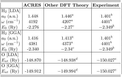
along a line through the centers of the two atoms. The enhancement of the grid resolution throughout the re-gions where the electronic wave functions are large and the very strong enhancement close to the nuclei allow accurate representation of the smooth tails of the wave functions as well as the cusps and nodes near the nuclei. For a more quantitative comparison to other theoret-ical results and to experiment, Table I shows our calcu-lated results for H2 and O. It is clear from this

compari-son that our results are in complete agreement with other theoretical work using similar methods. Therefore, the difference between calculated values and experimental measurements reflects fundamental limitations of the un-derlying theory (DFT/LDA or DFT/GGA), rather than limitations in the accuracy of our method.

The authors are grateful to F. Gygi for sharing his insight on adaptive methods. This work was supported by the Office of Naval Research grant N00014-93-1-0190.

[1] J. R. Chelikowsky, N. Troullier, and Y. Saad, Phys. Rev. Lett. 72, 1240 (1994); J. R. Chelikowsky, N. Troullier, K. Wu, and Y. Saad, Phys. Rev. B50, 11355 (1994). [2] E. L. Briggs, D. J. Sullivan, and J. Bernholc, preprint. [3] K. Cho, T. A. Arias, J. D. Joannopoulos, and P. K. Lam,

Phys. Rev. Lett.71, 1808 (1993).

[4] S. Q. Wei and M. Y. Chou, Bull. Amer. Phys. Soc.40, 43 (1995).

[5] E. Tsuchida and M. Tsukada, Sol. St. Comm. 94, 5 (1995).

[7] F. Gygi, Europhys. Lett.19, 617 (1992); Phys. Rev. B

48, 11692 (1993);51, 11190 (1995); Private communica-tion.

[8] D. R. Hamann, Phys. Rev. B51, 7337 (1995);51, 9508 (1995).

[9] A. Devenyi, K. Cho, T. A. Arias, and J. D. Joannopoulos, Phys. Rev. B49, 13373 (1994).

[10] P. Hohenberg and W. Kohn, Phys. Rev. 136, B864 (1964); W. Kohn and L. Sham,ibid.140, A1133 (1965). [11] J. P. Perdew, inElectronic Structure of Solids ’91, edited by P. Ziesche and H. Eschrig (Akademie Verlag, Berlin, 1991).

[12] Through our finite difference scheme, we have an approxi-mation of the original equations, rather than a projection of the original problem onto a basis. Consequently, the variational aspect of a basis is lost, and our electronic eigenvalues are not necessarily upper bounds of the true electronic eigenvalues.

[13] We caution the reader against a subtle but important pitfall in the error estimation of a numerical integral: the second Euler-Maclaurin summation formula is only an asymptotic formula. When applied to the case of a discretized integral of aC∞

periodic function, it leads to an obvious contradiction!

[14] P. J. Davis and P. Rabinowitz,Methods of Numerical In-tegration, 2nd ed. (Academic Press, Orlando, FL, 1984). [15] J. P. Perdew and A. Zunger, Phys. Rev. B 23, 5048

(1981).

[16] G. B. Bachelet, D. R. Hamann, and M. Schl¨uter, Phys. Rev. B26, 4199 (1982).

[17] L. Kleinman and D. M. Bylander, Phys. Rev. Lett.48, 1425 (1982).

[18] B. G. Johnson, P. M. W. Gill, and J. A. Pople, J. Chem. Phys.98, 5612 (1992).

[19] K. P. Huber and G. Herzberg, Molecular Spectra and Molecular Structure(Van Nostrand Reinhold Company, New York, 1979), Vol. IV.

[20] J. P. Perdewet al., Phys. Rev. B46, 6671 (1992). [21] Y.-M. Juan and E. Kaxiras, Phys. Rev. B 48, 14944

(1993); Private communication.

[22] C. E. Moore,Atomic Energy Levels (U. S. Government Printing Office, Washington, 1971), Vol. I.

FIG. 1. The 24×12×12 [a.u.] grid used for H2, in a horizontal cross-section through the atoms (every fourth line shown). Notice the effect of the global backdrop (crosslike pattern) and the local adaptation around each atom.

FIG. 2. Occupied wave functions of the O2molecule, along a line through the centers of the atoms. Theπ _{bonding and}

anti-bonding wave functions collapse onto the horizontal axis (they have nodes through the atomic centers). The 1s bond-ing and anti-bondbond-ing states were scaled by a factor of 1/3 so they could be displayed on the same scale. Points on the curves indicate values at actual grid points used in the calcu-lation.

TABLE I. Calculated bond length a0, vibrational fre-quency ω_{, and minimum energy} E0 for H2 and atomic en-ergy Eat of O. The zero-point vibrational energy has been subtracted from the experimental total energy of H2.

ACRES Other DFT Theory Experiment

H2 [LDA]

a0 (a.u.) 1.448 1.446 a

1.₄₀₁b

ω_(cm−1

) 4192 4207a

4401b

E0(Ry) -2.276 −2.27 c

−2.₃₄₉b H2 [GGA]

a0 (a.u.) 1.416 1.413 a

1.₄₀₁b

ω(cm−1

) 4381 4373a

4401b

E0(Ry) -2.340 ₋2.34 c

−2.349b O [LDA]

Eat(Ry) -148.870 ₋148.938 d

−150.027e O [GGA]

Eat(Ry) -149.912 −149.994 d

−150.027e

a _{Reference [18], S-VWN and B-LYP} b _{Reference [19]}

c _{Reference [20], LSD and PW GGA-II} d_{Reference [21], LDA and PW91}

e_{Reference [22], Spin unpolarized ground state, 2p}4 1

9

10

11

12

13

14

15

-3

-2

-1

0

1

2

3

Wavefunction