Determination of the ambient temperature in transient heat conduction.

This is a repository copy of Determination of the ambient temperature in transient heat

conduction..

White Rose Research Online URL for this paper:

http://eprints.whiterose.ac.uk/83756/

Version: Accepted Version

Article:

Hào, DN, Thanh, PX and Lesnic, D (2015) Determination of the ambient temperature in

transient heat conduction. IMA Journal of Applied Mathematics, 80 (1). 24 - 46. ISSN

0272-4960

https://doi.org/10.1093/imamat/hxt012

[email protected] https://eprints.whiterose.ac.uk/

Reuse

Unless indicated otherwise, fulltext items are protected by copyright with all rights reserved. The copyright exception in section 29 of the Copyright, Designs and Patents Act 1988 allows the making of a single copy solely for the purpose of non-commercial research or private study within the limits of fair dealing. The publisher or other rights-holder may allow further reproduction and re-use of this version - refer to the White Rose Research Online record for this item. Where records identify the publisher as the copyright holder, users can verify any specific terms of use on the publisher’s website.

Takedown

If you consider content in White Rose Research Online to be in breach of UK law, please notify us by

Determination of the ambient temperature in transient heat

conduction

Dinh Nho H`ao1,2_{, Phan Xuan Thanh}3 _{and D. Lesnic}2

1 _{Hanoi Institute of Mathematics, 18 Hoang Quoc Viet Road, Hanoi, Vietnam}

e-mail: [email protected]

2 _{Department of Applied Mathematics, University of Leeds, Leeds LS2 9JT, UK}

e-mails: [email protected], [email protected]

3_{School of Applied Mathematics and Informatics,}

Hanoi University of Science and Technology, 1 Dai Co Viet Road, Hanoi, Vietnam

e-mail: [email protected]

Abstract

The restoration of the space- or time-dependent ambient temperature entering a third-kind convective Robin boundary condition in transient heat conduction is investigated. The temper-ature inside the solution domain together with the ambient tempertemper-ature are determined from additional boundary measurements. In both cases of the space- or time-dependent unknown ambient temperature the inverse problems are linear and ill-posed. Least-squares penalised variational formulations are proposed and new formulae for the gradients are derived. Numer-ical results obtained using the conjugate gradient method combined with a boundary element direct solver are presented and discussed.

Keywords: Heat equation, ambient temperature, boundary element method, conjugate gradient method, inverse problem

1

Introduction

Further, in our study the unknown ambient temperature is allowed to vary with space or time. Therefore, a more realistic model can be proposed for the heat transfer in building enclosures, e.g. glazed surfaces, where the ambient temperature can vary spatially, or with time, depending on the local air patterns, e.g. type of flow, external weather conditions, etc., [16].

The plan of the paper is as follows. In Section 2 we formulate the inverse problems for the deter-mination of a space-dependent (Problem I) or time-dependent (Problem II) ambient temperature and recall the available existence and uniqueness results in the classical sense. Section 3 is devoted to defining the weak solutions of the direct and adjoint Robin problems and recalling their unique solvability. The symmetric Galerkin formulation of the boundary element method (BEM) given in [2] for the Dirichlet and Neumann direct problems is extended in Section 4 to the Robin problem for the transient heat equation. Furthermore, in our inverse problems, all the unknowns and additional observations are at the boundary and the discretization of the boundary only is the essence of the BEM. Therefore, it seems more natural and appropriate to use the BEM instead of the domain discretization methods such as the finite element or finite difference methods. Sections 5 and 6 are devoted to developing the least-squares variational methods for solving the inverse problems I and II, respectively. In each of these sections we present the numerical results for several benchmark test examples of interest obtained using the iterative conjugate gradient method (CGM) combined with the BEM direct solver. In all cases, numerical stability and good accuracy are achieved pro-vided that the iterative process is stopped according to the discrepancy principle. Finally, Section 7 presents the summary, conclusions and future work.

2

Mathematical formulation

Let Ω_∈Rd _{be a bounded domain and denote its boundary by Γ. In the cylinderQ:= Ω×(0, T],}

where T >0, with the lateral surface areaS = Γ_×(0, T], consider the following inverse problems ([8] and [9]). Throughout the paper,udenotes the temperature, f the ambient temperature,athe initial temperature,g the heat source, andσ the heat transfer coefficient.

Inverse Problem I.Find a pair of functions {u(x, t), f(ξ)} such that

ut−∆u=g inQ, (2.1)

u(x,0) =a(x), x∈Ω, (2.2)

∂u

∂n +σ(ξ, t)u=h(ξ, t)f(ξ) +b(ξ, t), (ξ, t)∈S, (2.3) l(u) =χ(ξ), ξ_∈Γ, (2.4)

where the functionsg(x, t), a(x), σ(ξ, t), h(ξ, t), b(ξ, t) andχ(ξ) are given, andnis the outward unit normal to the boundary Γ. Strictly speakingh should be equal toσ in order forf to represent the actual ambient temperature, but the boundary condition in (2.3) models a more general situation, which also include an additional heat flux contributionb(ξ, t). In (2.4), the observation operatorl

has one of the following forms:

l(u) =u(ξ, T1), ξ∈Γ, (2.5)

whereT1 is a fixed known time in (0, T], or

l(u) =

Z T

0

with ω being a given function in L1(0, T). The additional conditions (2.5) and (2.6) are called terminal and integral boundary observations, respectively.

Inverse Problem II. Find a pair of functions_{u(x, t), f(t)_} such that

ut−∆u=g inQ, (2.7)

u(x,0) =a(x), x_∈Ω, (2.8)

∂u

∂n +σ(ξ, t)u=h(ξ, t)f(t) +b(ξ, t), (ξ, t)∈S, (2.9) l1(u) =χ1(t), t∈[0, T], (2.10)

where the functionsg(x, t), a(x), σ(ξ, t), h(ξ, t), andχ1(t) are given. The observation operatorl1(u)

has one of the following forms:

l1(u) =u(ξ0, t), t∈[0, T], (2.11)

whereξ0 is fixed known point in Γ, or

l1(u) =

Z

Γ

ν(ξ)u(ξ, t)dξ, t_∈[0, T], (2.12)

with ν(ξ) being a given function in L1(Γ). The additional conditions (2.11) and (2.12) are called point and boundary integral observations, respectively.

At this stage, it is worth mentioning that in practice conditions (2.6) and (2.12) are indeed measured by averaging a series of pointwise boundary temperature measurements. This is particularly ad-vantageous to use in situations where the time pointwise or space pointwise boundary temperature measurements (2.5) or (2.6) posses different sensitivities with respect to the value ofT1 within the

interval (0, T] or, the boundary pointξ0along the boundary Γ, respectively. On the other hand, one

can observe that equations (2.6) and (2.12) reduce to equations (2.5) (for T1 ∈(0, T)) and (2.11)

if one takes the weights ω(t) =δ(t−T1) and ν(ξ) = δ(ξ−ξ0), respectively, where δ is the Dirac

delta function. However, because ω and ν have to be L1-integrable, these choices are not quite strictly possible. Approximations with Gaussian functions or employing cut-off weights, see later equations (5.1) and (6.1), can be alternatives to model pointwise measurements (thermocouples have non-zero width, or the time is never instant) as local averages.

The common feature in the above inverse problems is the Robin third kind boundary condition, see equations (2.3) and (2.9).

The notation for the spaces of functions involved in the following theorems follows [7]. With the assumptions that Ω is simply-connected and its boundary Γ∈C1+β with β >0, g∈Cβ,0(Q), a∈

C1(Ω), h, b∈C(S), Kostin and Prilepko [8, 9] proved the following results.

Theorem 2.1. Suppose that σ is independent of t, σ _∈C(Γ), 0 _≤σ(ξ) onΓ, ω(t) _≥0 on [0, T],

l(h) > 0 almost everywhere on Γ, and the function h is positive on S, monotone non-decreasing with respect to t. Then the solution (u(x, t), f(ξ)) ∈ C2,1(Q)×C(Γ) to the inverse problem I is unique.

Theorem 2.2. Assume σ _∈ C(S) and denote by u0 _{∈ C}2,1_(Q)∩Cβ,β/2_{(Q) the unique solution} of the direct problem (2.7)–(2.9) with f = 0 (see [7]). Further, assume that the function χ2(t) :=

χ1(t)−l1(u0) ∈ C1/2[0, T] and χ2(0) = 0,_dtd

Rt

0 χ2(τ)

√

t−τdτ ∈ C[0, T]. Then, if h ∈ C

Although of theoretical interest, these uniqueness theorems cannot be used directly in the numerical analysis, since it is not straightforward how to use the space of continuous functions in a weak formulation. Therefore, in this paper we relax some assumptions on the smoothness of the data posed above so that we can work in the Hilbert space framework. Then we can solve the above inverse problems in the least-squares sense. We will report about this in the next section.

3

Direct problem

In this section, we suppose that Ω is a bounded Lipschitz domain and introduce the notion for standard Sobolev spaces as follows.

For a Banach spaceB, we define

L2(0, T;B) ={u:u(t)∈B a.e.t∈(0, T) and kukL2_(0,T;B)<∞},

with the norm

kuk2L2_(0,T;B)=

Z T

0 k

u(t)k2Bdt.

In the sequel, we shall use the spaceW(0, T) defined as

W(0, T) ={u:u∈L2(0, T;H1(Ω)), ut∈L2(0, T; (H1(Ω))′)},

equipped with the norm

ku_k2_W(0,T) =_ku_k2_L2_(0,T;H1_(Ω))+ku_tk2_L2_(0,T;(H1_(Ω))′₎.

Now consider the direct problem

ut−∆u=g inQ, (3.1)

u(x,0) =a(x), x_∈Ω, (3.2)

∂u

∂n +σ(ξ, t)u=b(ξ, t), (ξ, t)∈S, (3.3)

with

g∈L2(Q), a∈L2(Ω), σ∈L∞(S), σ≥0, b∈L2(S). (3.4)

Definition 3.1. A functionu∈W(0, T) is called a weak solution to the direct problem (3.1)–(3.3), if

Z

Q

(utη+∇u· ∇η)dxdt+

Z

S

σuηdξdt=

Z

Q

gηdxdt+

Z

S

bηdξdt (3.5)

for all η∈L2(0, T;H1(Ω)), and u(·,0) =a.

The following theorem giving the existence and uniqueness of a weak solution to the direct problem (3.1)–(3.3) is given in [15].

Theorem 3.2. Suppose that conditions(3.4)are satisfied. Then there exists a unique weak solution in W(0, T) of the direct problem (3.1)–(3.3). Moreover, there exists a constant cd>0 independent of g, b and asuch that

Remark 3.3. The constant cd depends on σ. However, if we suppose that

0< σ1≤σ≤σ2,

where σ1 andσ2 are given, then by examining the proof of this theorem in [10] and [15] we see that

cd depends on these two constants only.

We introduce now the adjoint problem to (3.1)–(3.3) as follows:

−ψt−∆ψ=aQ inQ, (3.7)

ψ(x, T) =aΩ(x), x∈Ω, (3.8)

∂ψ

∂n +σ(ξ, t)ψ=aS(ξ, t), (ξ, t)∈S, (3.9)

with

aQ∈L2(Q), aΩ ∈L2(Ω), σ∈L2(S), σ≥0, aS ∈L2(S). (3.10)

From Lemma 3.17 and Theorem 3.18 in [15] we have the following theorem giving the existence and uniqueness of a weak solution to the adjoint problem (3.7)–(3.9).

Theorem 3.4. Suppose that conditions (3.10) are satisfied. Then there exists a unique weak solution in W(0, T) of the adjoint problem (3.7)–(3.9) in the sense that

Z

Q

(₋ψtη+∇ψ· ∇η)dxdt=

Z

Q

aQηdxdt+

Z

S

aSηdξdt−

Z

S

σψηdξdt

for allη∈L2(0, T;H1(Ω)), andψ(·, T) =aΩ(·). Moreover, there exists a constantca>0 indepen-dent of aQ, aΩ andaS such that

kψ_{kW(0,T) ≤}ca(kaQkL2_(Q)+ka_Sk_L2_(S)+ka_Ωk_L2_(Ω)). Furthermore, ifu_∈W(0, T) is the weak solution to the problem (3.1)–(3.3), then

Z

Ω

aΩ(x)u(x, T)dx+

Z

Q

aQudxdt+

Z

S

aSudξdt

=

Z

Ω

a(x)ψ(x,0)dx+

Z

Q

gψdxdt+

Z

S

bψdξdt.

(3.11)

4

Boundary element method for the direct problem

The unknown Cauchy data [w := ∂u

∂n, u] on S of the direct problem (3.1)–(3.3) with the input

data satisfying (3.4) can be found by the boundary integral equation approach of [2]. Indeed, the solution of the heat equation (3.1) is given by a representation formula, for (˜x, t)_∈Q,

u(˜x, t) =

t

Z

0

Z

Γ

E(˜x₋y, t₋τ)w(y, τ)dsydτ − t

Z

0

Z

Γ

∂_E

∂ny

(˜x₋y, t₋τ)u(y, τ)dsydτ

+

Z

Ω

E(˜x−y, t)a(y)dy+

t

Z

0

Z

Ω

whereE(x, t) is the fundamental solution of the heat equation as given in [2]:

E(x, t) =

 



(4πt)−d2e−

|x|2

4t fort >0,

0 fort_≤0.

We define the single and double layer heat potentials as

(V w)(x, t) =

t

Z

0

Z

Γ

E(x−ξ, t−τ)w(ξ, τ)dξ dτ, (Ku)(x, t) =

t Z 0 Z Γ ∂

∂nξE

(x−ξ, t−τ)u(ξ, τ)dξ dτ,

for (x, t)_∈S, and the boundary integral operators N and W,

(N w)(x, t) =

t Z 0 Z Γ ∂

∂nxE

(x₋ξ, t₋τ)w(ξ, τ)dξ dτ,

and

(W u)(x, t) =− ∂

∂nx t Z 0 Z Γ ∂

∂nξE

(x−ξ, t−τ)u(ξ, τ)dξ dτ

as in [2]. Moreover, we introduce the volume potentials, for (x, t)_∈S,

(M0a)(x, t) =

Z

Ω

E(x−y, t)a(y)dy, (N0g)(x, t) = t

Z

0

Z

Ω

E(x−y, t−τ)g(y, τ)dy dτ

and

(_M1a)(x, t) =

∂

∂nx

Z

Ω

E(x₋y, t)a(y)dy, (_N1g)(x, t) =

∂ ∂nx t Z 0 Z Ω

E(x₋y, t₋τ)g(y, τ)dy dτ.

For the properties of the above operators, see [2, 14]. In particular, we have thatN is the adjoint of the double layer potentialK with respect to the ”time-twisted” duality, see [2, p.541], i.e.,

hκTw, N ϕi=hκTϕ, Kwi,

where the time reversal mapκT is defined by κTv(x, t) :=v(x, T −t).

As in [2], we obtain the boundary integral equations

(V w)(x, t) =

µ

1 2I+K

¶

u(x, t)−(M0a)(x, t)−(N0g)(x, t) for (x, t)∈S, (4.2)

and

(W u)(x, t) =

µ

1 2I−N

¶

w(x, t)₋(_M1a)(x, t)−(N1g)(x, t) for (x, t)∈S. (4.3)

From the boundary condition (3.3), we are now in a position to rewrite the boundary integral equations (4.2) and (4.3) as follows:

A Ã w u ! := Ã

V ₋¡₁

2I+K

¢

¡₁

2I+N

¢

W +σI

! Ã w u ! = Ã

−M0a− N0g

b_{− M}1a− N1g

!

Lemma 4.1. The operator A is elliptic, i.e., ­ A Ã w u ! , Ã w u ! ® =­ Ã

V −K

N W ! Ã w u ! , Ã w u ! ®

+_hσu, u_{i ≥}C

µ

kw_k2

H−12,− 1

4_(S)+kuk 2 H12,

1 4_(S)

¶

for all w_∈H−12,− 1

4(S),u∈H 1 2,

1

4(S) and some positive constantC.

Proof. See [2, Theorem 3.11] and use the conditionσ _≥0.

By assumptions (3.4), the boundary integral equations (4.4) admit a unique solution (w, u) _∈

H−12,− 1

4(S)×H 1 2,

1

4(S). Let us consider now the numerical discretization of (4.4).

LetVh be the trial space of functions which are piecewise linear with respect to the space variables

on a triangulation of Γ and piecewise constant with respect to the time variable. We also introduce a set of ansatz functions _Uh consisting of piecewise constant basis functions both in space and in

time, see [2, 14].

The Galerkin variational formulation of (4.4) is to find (wh, uh)∈ Vh× Uh such that

­ A Ã wh uh ! , Ã τh vh ! ® =­ Ã

−M0a− N0g

b− M1a− N1g

! , Ã τh vh ! ®

for all (τh, vh)∈ Vh× Uh.

This is equivalent to

(­

V wh, τh

®

S−

­ ¡₁

2I+K

¢ uh, τh

®

S =−

­

M0a+N0g, τh

®

S,

­ ¡₁

2I+N

¢ wh, vh

®

S+

­

W uh, vh

®

S+

­

σuh, vh

®

S =

­

b_{− M}1a− N1g, vh

®

S,

(4.5)

for all (τh, vh)∈ Vh× Uh.

Let

uh(x, t) =

n−1

X

ℓ=0 m1−1

X

i=0

uiℓϕ1i(x)ψℓ0(t), wh(x, t) = n−1

X

ℓ=0 m0−1

X

j=0

wjℓϕ0j(x)ψℓ0(t).

Here,m0 =m1in two dimensional case,nis the number of time steps,ϕ0j(x) andϕ1i(x) are piecewise

constant and piecewise linear basis functions in space, respectively, andψ0_ℓ(t) are piecewise constant basis functions in time.

With these approximations we obtain the following linear system of equations:

(

Vhw−(1₂Mh+Kh)u=f1

(1₂M⊤

h +Nh)w+Whu+Mhσu=f2

whereVh, Kh, Nh andWh are the Galerkin matrices corresponding to the boundary integral

opera-tors V, K, N andW, andMh is the mass matrix, see [5, 14]. The vectorsf1 and f2 are the related

vectors to the right hand sides.

Moreover, we introduce the mass matrix entries

M_kℓσ[j][i] =_hσ(x, t)ϕ1_i(x)ψ0_ℓ(t), ϕ1_j(x)ψ0_k(t)_i=

T

Z

0

Z

Γ

σ(x, t)ϕ1_i(x)ψ_ℓ0(t)ϕ1_j(x)ψ_k0(t)dsxdt,

which are zero whenever k₆=ℓ. Fork=ℓ, we denote the matrixMσ

Note that the matrix 1₂M_h⊤+Nh can be obtained as follows. We first have the following (block)

lower triangular matrices:

Vh =

       V0

V1 V0

... ... ...

Vn−2 Vn−3 V0

Vn−1 Vn−2 V0

      

, Wh=

       W0

W1 W0

... ... ...

Wn−2 Wn−3 W0

Wn−1 Wn−2 W0

       1

2Mh+Kh =

       K0

K1 K0

... ... ...

Kn−2 Kn−3 K0

Kn−1 Kn−2 K0

       and then 1

2Mh⊤+Nh=

       K⊤ 0 K⊤

1 K0⊤

... ... ...

K⊤

n−2 Kn⊤−3 K0⊤

K⊤

n−1 Kn⊤−2 K0⊤

       .

The linear system

Ã

Vh −(12Mh+Kh)

(1₂M⊤

h +Nh) Wh+Mhσ

! Ã w u ! = Ã f1 f2 !

can be rewritten as follows:

       V0

V1 V0

... ... ...

Vn−2 Vn−3 V0

Vn−1 Vn−2 V0

              w0 w1 ...

wn−2

wn−1

       −        K0

K1 K0

... ... ...

Kn−2 Kn−3 K0

Kn−1 Kn−2 K0

              u0 u1 ... un−2

un−1

       =        f1 0 f1 1 ... f_n1₋₂ f_n1₋₁

       and       

K₀⊤

K₁⊤ K₀⊤

... ... ...

K_n⊤₋₂ K_n⊤₋₃ K₀⊤

K_n⊤₋₁ K_n⊤₋₂ K₀⊤

              w0 w1 ...

wn−2

wn−1

       + +       

W0+M0σ

W1 W0+M1σ

... ... ...

Wn−2 Wn−3 W0+Mnσ−2

Wn−1 Wn−2 W0+Mnσ−1

              u0 u1 ... un−2

un−1

       =        f2 0 f2 1 ... f2

n−2

f2

n−1

       .

From the first two equations of the above systems, we obtain

Ã

V0 −K0

K₀⊤ W0+M0σ

! Ã w0 u0 ! = Ã f₀1 f₀2

!

=⇒hK₀⊤V₀−1K0+W0+M0σ

i

u0 =f02−K0⊤V0−1f01,

since the matrix V0 is invertible, and then we can solve for u0 and w0. Therefore, wk and uk can

be found from the system

(

Vkw0+Vk−1w1+...+V0wk−Kku0−Kk−1u1−...−K0uk=f_k1

fork= 1, ..., n−1. This system can be re-arranged as follows:

(

V0wk−K0uk=f_k1+Kku0+Kk−1u1+...+K1uk−1−Vkw0−Vk−1w1−...−V1wk−1

K₀⊤wk+ (W0+M_kσ)uk=fk2−Kk⊤w0−...−K1⊤wk−1−Wku0−...−W1uk−1.

Observe that the matricesRm1×m1 ∋Ak_h :=K₀⊤V₀−1K0+W0+Mkσ,k= 0, ..., n−1, are symmetric

and positive definite and the corresponding system of linear equations can be solved efficiently using standard methods of inversion.

5

Variational method for the inverse problem I

Now we return to the inverse problem I consisting of determining {u(x, t), f(ξ)} from the system of equations (2.1)–(2.4). If we suppose that g ∈ L2(Q), a ∈ L2(Ω), h ∈ L∞(S), f ∈ L2(Γ), b ∈

L2(S) and σ ∈ L∞(S), σ ≥0, then from Theorem 3.2, there exists a unique solution in W(0, T) of the direct problem (2.1)–(2.3). Since u ∈ W(0, T), we cannot determine the trace u(ξ, T1),

ξ∈Γ,0< T1 ≤T in (2.5). Therefore, in this setting, we take the observation operatorlas in (2.6).

Afterwards we use

1

γ Z T1

T1−γ

u(ξ, t)dt, (5.1)

whereγ >0 small, as an approximation tou(ξ, T1), if it exists. Here and thereafter, for simplicity,

we suppose that the weightω∈L2(0, T).

To emphasize the dependence of the solution u of (2.1)–(2.3) on the boundary dataf, sometimes we write it byu(x, t;f) oru(f). Now, the variational approach to the first inverse problem can be considered as the problem of minimizing the functional

Jα(f) =

1 2

Z

Γ

³Z T

0

ω(t)u(ξ, t;f)dt₋χ(ξ)´2dξ+α

2kfk

2 L2_(Γ)

= 1 2

Z

Γ|

l(u(f))₋χ_|2dξ+α

2kfk

2

L2_(Γ) (5.2)

overL2_{(Γ), where u(x, t;f) solves (2.1)–(2.3) andα is the regularization parameter.}

Since the mapping from f _∈ L2(Γ) to l(u) is affine, by the standard reasoning, we see that the above minimization problem admits a unique solution, ifα >0.

We note that since the imbedding of the trace ofW(0, T) onS intoL2(0, T;L2(Γ)) is compact, the mapping fromf ∈L2(Γ) to l(u(f))∈L2(Γ) is compact. Hence the inverse problem in this setting is ill-posed and so is the minimization problem forJ0.

Now we find the gradient ofJα.

Take a variationδf ∈L2(Γ) and consider problem (2.1)–(2.3) with the data f +δf instead of f. We have the unique solutionu(x, t;f+δf)∈W(0, T).

Setv=u(x, t;f+δf)₋u(x, t;f). Then, v_∈W(0, T) is the weak solution of

vt−∆v= 0 in Q, (5.3)

v(x,0) = 0, x_∈Ω, (5.4)

∂v

We have

J0(f+δf)−J0(f) =

1 2

Z

Γ

³Z T

0

ω(τ)¡

u(ξ, τ;f) +v(ξ, τ;δf)¢

dτ₋χ(ξ)´2dξ

− 1

2

Z

Γ

³Z T

0

ω(τ)u(ξ, τ;f)dτ−χ(ξ)´2dξ

=

Z

Γ

³Z T

0

ω(τ)v(ξ, τ;δf)dτ´³

Z T

0

ω(τ)u(ξ, τ;f)dτ₋χ(ξ)´dξ

+ 1 2

Z

Γ

³Z T

0

ω(τ)v(ξ, τ;δf)dτ´2dξ.

To evaluate the first item in the last equation, we introduce the adjoint problem

−ψt−∆ψ= 0 in Q, (5.6)

ψ(x, T) = 0, x∈Ω, (5.7)

∂ψ

∂n +σ(ξ, t)ψ=ω(t)

³Z T

0

ω(τ)u(ξ, τ)dτ₋χ(ξ)´ on S. (5.8)

There exists a unique weak solution in W(0, T) of this problem and applying Theorem 3.4 to (5.3)–(5.5) and (5.6)–(5.7), we have that the identity (3.11) yields

Z

S

³Z T

0

ω(τ)u(ξ, τ;f)dτ−χ(ξ)´ω(t)v(ξ, t)dξdt=

Z

S

h(ξ, t)δf(ξ)ψ(ξ, t)dξdt

=

Z

Γ

³Z T

0

ω(t)u(ξ, t;f)dt₋χ(ξ)´³

Z T

0

ω(t)v(ξ, t)´dξ. (5.9)

On the other hand, in virtue of Theorem 3.2,

kvkW(0,T)≤cdkhkL∞_(Q)kδfk_L2_(Γ).

Hence

J0(f +δf)−J0(f) =

Z

S

h(ξ, t)ψ(ξ, t)δf(ξ)dξdt+o(kδfkL2_(Γ)).

Thus, we conclude that the functionalJ0 is Fr´echet differentiable and its gradient has the form

J₀′(f) =

Z T

0

h(ξ, t)ψ(ξ, t)dt. (5.10)

We immediately have

J_α′(f) =

Z T

0

h(ξ, t)ψ(ξ, t)dt+αf. (5.11)

Thus, the optimality condition for the problem (5.2), (2.1)–(2.3) is

Z T

0

h(ξ, t)ψ(ξ, t)dt+αf = 0. (5.12)

5.1 Boundary element method for the variational problem

Denoting the solution of the direct problem (2.1)–(2.3) with f = 0 by u0 and that withg= 0, a=

0, b= 0 by ¯u, then the solution of (2.1)–(2.3) isu =u0+ ¯u. The operator A0f =l(¯u(f)) is linear

and bounded, and the operator Af = l(u(f)) = A0f +l(u0) is affine. Thus, the functional (5.2)

can be written in the form

Jα(f) =

1

2kAf −χk

2 L2_(Γ)+

1 2αkfk

2 L2_(Γ)

= 1

2kA0f −(χ−l(u0))k

2 L2_(Γ)+

1 2αkfk

2 L2_(Γ)

:= 1

2kA0f−χk

2 L2_(Γ)+

1 2αkfk

2 L2_(Γ).

It follows that the gradient ofJα can be represented as

J_α′(f) =A∗₀(Af−χ) +αf. (5.13) Here A∗₀ :L2(Γ)→L2(Γ) is the adjoint operator ofA0 defined byA∗0q=

RT

0 h(ξ, t)ψ(ξ, t)dt, where

ψ is the solution of the adjoint problem

−ψt−∆ψ= 0 in Q, (5.14)

ψ(x, T) = 0, x∈Ω, (5.15)

∂ψ

∂n +σ(ξ, t)ψ=ω(t)q(ξ), (ξ, t)∈S. (5.16)

Now, the optimality condition (5.12) can be rewritten in the form

A∗₀(Af ₋χ) +αf= 0, (5.17)

from which we see immediately that there exists a unique solutionfα of it, ifα >0.

Using the ansatz functions_Vh× Uh as described in Section 4 with mesh sizehin space variable and ∼√h in time variable, we can derive the error estimate

ku−uhkL2_(Γ)≤chkfk_L2_(Γ) (5.18)

withc being a positive constant. Defining

A0,hf =

Z T

0

ω(t)uh(ξ, t;f)dt,

we conclude that

kA0f−A0,hfkL2_(Γ) ≤chkfk_L2_(Γ).

Hence the discrete version of the optimal control problem (5.2), (2.1)–(2.3) reads

min

f∈L2_(Γ)

³1

2kA0,hf−χk

2 L2_(Γ)+

α

2kfk

2 L2_(Γ)

´

(5.19)

which is characterized by the first-order optimality condition

Here A∗_0,h:L2(Γ)→L2(Γ) is the adjoint operator of A0,h defined by

A∗_0,h(A0,hfh−χ) =

RT

0 h(ξ, t)ψ(ξ, t)dt, whereψ is the solution of the adjoint problem

−ψt−∆ψ= 0 in Q, (5.21)

ψ(x, T) = 0, x_∈Ω, (5.22)

∂ψ

∂n +σ(ξ, t)ψ=ω(t)(A0,hfh−χ)(ξ), (ξ, t)∈S. (5.23)

If we solve the last problem by the BEM, then we get an approximation ˆA∗_0,h of A∗_0,h for which

kA∗_0,h−Aˆ∗_0,hk ≤ch. (5.24) Thus, we arrive at the variational problem

ˆ

A∗_0,h(A0,hfˆhα−χǫ) +αfˆhα = 0 (5.25)

with a perturbationχ_ǫ of χ satisfying

kχ−χ_ǫkL2_(Γ)≤ǫ. (5.26)

By the same technique as in the proof of Theorem 1 in [5] we can prove that if fα _{is the solution}

of the problem (5.12) and α >0, then

kfα−fˆ_hαkL2_(Γ)≤c(h+ǫ) (5.27)

withc being a constant depending onfα_{, χandα.}

5.2 Conjugate gradient method for problem (2.1)–(2.4)

1. Initialization

1.1. Choose an initial guess f0∈L2(Γ).

1.2. Calculate the residual ˜r0 =Ahf0−χǫ by solving the direct problem (2.1)–(2.3) with f =f0

by BEM.

1.3. CalculateJα(f0) = 1₂kr˜0k2+α₂kf0k2.

1.4. Calculate the gradient r0 by solving the adjoint problem (5.14)–(5.16) withq = ˜r0 and set

r0=

Z T

0

h(ξ, t)ψ0(ξ, t)dt+αf0.

1.5. Defined0 =−r0.

2. Forn= 1,2, . . .

2.1. Solve (2.1)–(2.3) with g= 0, a= 0, b= 0 and f =dn for calculatingA0,hdn. Calculate

αn= k

rnk2

kA0,hdnk2+αkdnk2

.

2.2. Updatefn+1=fn+αndn.

2.4. Calculate the gradient rn+1 by solving the adjoint problem (5.14)–(5.16) with q = ˜rn+1 and

set

rn+1 =

Z T

0

h(ξ, t)ψn+1(ξ, t)dt+αfn+1.

2.5. Jα(fn+1) = 1₂kr˜n+1k2+1₂αkfn+1k2.

2.6. βn= krn+1k 2

krnk2 .

2.7. Updatedn+1 =−rn+1+βndn.

When α= 0, stop at the firstnsuch that_k˜rnk ≤γ1ǫ, whereγ1 is some number greater than 1, or

when_krnk< ǫ. This discrepancy principle stopping criterion is required in order to achieve a stable

solution, [11]. We can also choose α > 0 as the regularization parameter in Tikhonov’s method and stop the algorithm with a tolerance error. Of course, as the CGM is in itself a regularizing method, there is, in principle, no need to include a regularization term in the functional (5.2) that is minimized. As recently investigated in [5], both methods with or without α included produce similar results. However, the choice of γ1 > 1 in the CGM with α = 0 is not obvious

and moreover, the inclusion of α > 0 in the CGM tends to achieve a more robust stability than when α = 0. Finally, we mention that the Tikhonov functional (5.2) with α >0 is recommended when used in conjunction with other iterative algorithms for minimization which do not necessarily have a regularizing effect. This is because otherwise, when α = 0, stopping the iterations at a threshold given by the discrepancy principle, for example, does not guarantee that a stable solution is obtained.

5.3 Numerical examples

The one-dimensional spacewise ambient temperature case has been numerically investigated at length in [13] and therefore, in this subsection the emphasis is put on the multi-dimensional (two-dimensional) framework. We consider three examples in decreasing order of smoothness, namely: smooth, piecewise smooth and discontinuous functions.

In all examples in this subsection, Ω = (0,1)_×(0,1), T = 1, g = 0, a = 0, σ(ξ, t) = ξ₁2+ξ₂2 + 1, h(ξ, t) = ξ1+ξ2+ sin(₂t + 1), where ξ = (ξ1, ξ2). For the temperature we take the exact solution

be given by, see [2],

u(x, t) = 100

4πte

−|x−x0|2

4t , (5.28)

wherex0= (−1,−1). Then prescribingf we can take bgiven by

b(ξ, t) := ∂u

∂n +σ(ξ, t)u−h(ξ, t)f(ξ), (ξ, t)∈S. (5.29)

The measurement (2.4) is obtained directly from (5.28), via (2.6) or (5.1). In the case of the integral measurement (2.6) we take ω(t) =t2+ 1. In the case of the terminal-integral measurement (5.1),

γ = 10−5 is fixed throughout, and the terminal timeT1 is varied within the interval (0, T].

In order to investigate the stability of the numerical solution we add noise to the measurement (2.4), as

χnoisy =χ+ǫ×rand(1), (5.30)

The number of boundary elements is taken as M = 256 and the number of time steps is taken as

N = 128. These numbers are found sufficiently large to ensure that any further increase in them did not significantly affect the accuracy of the numerical results.

For simplicity, we illustrate the results obtained withα= 0 and the CGM stopped according to the discrepancy principle withγ1 = 1.05 starting with the initial guessf0 = 0. We have also tested the

unstopped CGM, but regularized with a positiveα such as α = 10−5, and we have found similar results. Therefore, these latter results are not illustrated.

We aim to retrieve the following functions representing the spacewise dependent ambient temper-ature:

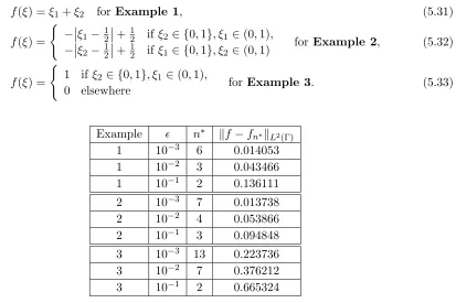
f(ξ) =ξ1+ξ2 forExample 1, (5.31)

f(ξ) =

(

−¯ ¯ξ₁−1

2

¯ ¯+1

2 ifξ2 ∈ {0,1}, ξ1 ∈(0,1), −¯

¯ξ₂−1

2

¯ ¯+1

2 ifξ1 ∈ {0,1}, ξ2 ∈(0,1)

forExample 2, (5.32)

f(ξ) =

(

1 if ξ2∈ {0,1}, ξ1 ∈(0,1),

0 elsewhere forExample 3. (5.33)

Example ǫ n∗ _kf₋fn∗k_L2_(Γ)

1 10−3 6 0.014053 1 10−2 3 0.043466 1 10−1 2 0.136111 2 10−3 7 0.013738 2 10−2 4 0.053866 2 10−1 _{3 0.094848}

3 10−3 13 0.223736 3 10−2 _{7 0.376212}

3 10−1 2 0.665324

Table 1: The stopping CGM iteration numbersn∗ and theL2(Γ)-errors_kf₋fn∗k_L2_(Γ)for Examples

1–3 of the inverse problem I with the integral observation (2.6) perturbed by various levels of noise

ǫ_{∈ {}10−3,10−2,10−1_}.

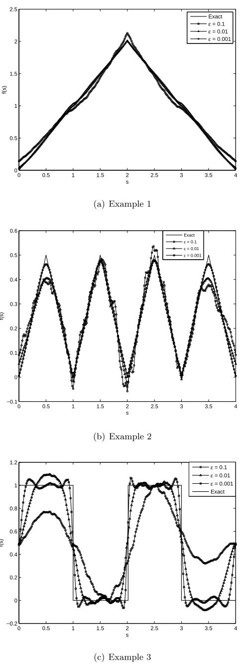
Figure 1 shows the the comparison between the exact and numerical solutions of the inverse problem I with the integral observation (2.6) perturbed by various levels of noiseǫ∈ {10−3,10−2,10−1}for Examples 1–3. These levels of noise yield the stopping CGM iteration number n∗ and the L2 (Γ)-errorskf−fn∗k_L2_(Γ)given in Table 1. From Figure 1 and Table 1 it can be seen that the numerical

solutions for all three Examples 1–3 are stable and they become more accurate as the level of noise

ǫ decreases. Obviously, Examples 2 and 3 are more difficult to retrieve accurately because the functions (5.32) and (5.33) are less regular than the smooth function (5.31). Finally, the low values of the stopping iteration numbersn∗ _{reported in Table 1 show that the CGM rapidly achieves the}

required level of stability and accuracy.

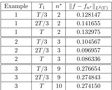
Next we discuss the numerical results obtained for the inverse problem I with the terminal obser-vation (2.5). As previously mentioned at the beginning of Section 5, since the trace (2.5) is not defined for the weak solution, we use instead the measurement (5.1), which is of the integral type (2.6) with

ω(t) =

(

1

γ, ift∈[T1−γ, T1],

Example T1 n∗ kf −fn∗k_L2_(Γ)

1 T /3 2 0.128147 1 2T /3 2 0.141655

1 T 2 0.132975

2 T /3 3 0.104567 2 2T /3 3 0.096957

2 T 3 0.086336

3 T /3 9 0.276654 3 2T /3 9 0.274843

3 T 10 0.274150

Table 2: The stopping CGM iteration numbersn∗ _{and theL}2_{(Γ)-errorskf−f}

n∗k_L2_(Γ)for Examples

1–3 of the inverse problem I with terminal-integral observation (5.1) perturbed byǫ= 10−1 _noise

for Example 1, ǫ = 10−2 _{noise for Example 2, and ǫ = 10}−3 _{noise for Example 3, for various}

terminal timesT1∈ {T /3,2T /3, T}.

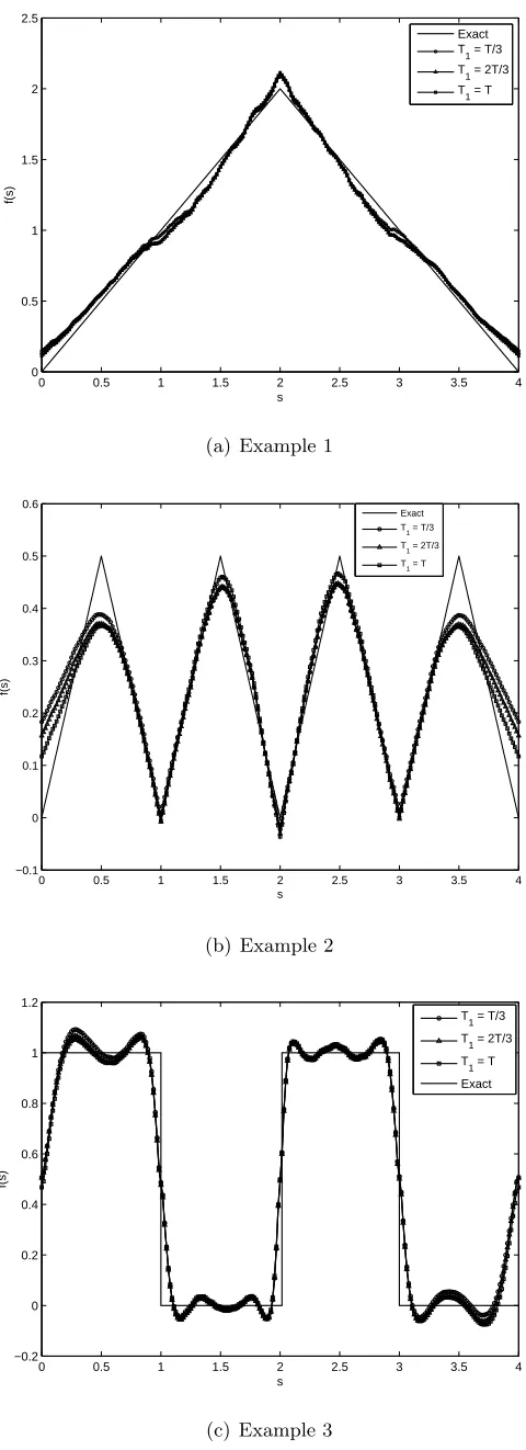
Letting γ > 0 small, such as γ = 10−5, we expect (5.1) to become a good approximation to (2.5). Figure 2 shows the comparison between the exact and numerical solutions for the spacewise dependent ambient temperature of the inverse problem I with the terminal-integral observation (5.1), withγ = 10−5, perturbed by ǫ= 10−2 noise for various terminal times T1 ∈ {T /3,2T /3, T}

for Examples 1-3. The stopping CGM iteration numbers n∗ and the L2(Γ)-errors kf −fn∗k_L2_(Γ)

are given in Table 2. From Figure 2 and Table 2 it can be seen that the numerical solutions for all three Examples 1–3 are stable and they are quite insensitive to the choice of the terminal timeT1.

6

Variational method for the inverse problem II

As in Section 5, since u ∈ W(0, T) we cannot determine the trace u(ξ0, t), t ∈ [0, T], ξ0 ∈ Γ in

(2.11). Therefore, in this setting, we take the observation operatorl1 as in (2.12). Afterwards, we

use

1 2γ

Z

Γ(ξ0,γ)={ξ∈Γ||ξ−ξ0|≤γ}

u(ξ, t)dξ, (6.1)

whereγ >0 is small, as an approximation tou(ξ0, t), if it exists. Here and thereafter, for simplicity

we suppose that the weightν _∈L2_(Γ).

The variational setting of the inverse problem II given by equations (2.7)–(2.10) and (2.12) is as follows.

Minimize the functional

Jα(f) =

1

2kl1(u(f)−χ1k

2

L2_(0,T)+

α

2kfk

2 L2_(0,T)

= 1 2

Z T

0

¯ ¯ ¯ Z

Γ

ν(ξ)u(ξ, t;f)dξ₋χ1(t)

¯ ¯ ¯

2

dt+α

2kfk

2

L2_(0,T), (6.2)

where u = u(x, t;f) is the solution in W(0, T) of the problem (2.7)–(2.9) with g ∈ L2(Q), a ∈

L2(Ω), σ∈L∞(S), σ≥0, h∈L2(S), ν ∈L2(Γ), and χ1∈L2(0, T) being given.

There exists a unique solution in W(0, T) of problem (2.7)–(2.9) for f _∈ L2_{(0, T), therefore, the}

By the same arguments in the variational method for the inverse problem I, as described in Section 5, we can prove that there exists a solution of this minimization problem, the functional (6.2) is Fr´echet differentiable and ifψ is the solution of the adjoint problem

−ψt−∆ψ= 0 in Q, (6.3)

ψ(x, T) = 0, x∈Ω, (6.4)

∂ψ

∂n +σ(ξ, t)ψ=ν(ξ)

³Z

Γ

ν(ξ)u(ξ, t;f)dξ−χ1(t)

´

, (ξ, t)∈S, (6.5)

then

J₀′(f) =

Z

Γ

h(ξ, t)ψ(ξ, t)dξ.

and

J_α′(f) =J₀′(f) +αf.

Denote the solution the direct problem (2.7)–(2.9) withf = 0 byu0and that withg= 0, a= 0, b= 0

by ¯u, then the solution of (2.7)–(2.9) is u = u0 + ¯u. The operator A0f = l1(¯u(f)) is linear and

bounded, and the operatorAf =l(u(f)) =A0f +l1(u0) is affine.

6.1 Conjugate gradient method for problem (6.2), (2.7)–(2.9)

1. Initialization

1.1. Choose an initial guess f0∈L2(0, T).

1.2. Calculate the residual ˜r0 =Af0−χǫ by solving the direct problem (2.7)–(2.9) withf =f0.

1.3. CalculateJα(f0) = 1₂kr˜0k2+α₂kf0k2.

1.4. Calculate the gradientr0 by solving the adjoint problem (6.3)–(6.5) with the right hand side

of (6.5) equal toν(ξ)˜r0 and set

r0 =

Z

Γ

h(ξ, t)ψ0(ξ, t)dξ+αf0.

1.5. Defined0 =−r0.

2. Forn= 1,2, . . .

2.1. Solve (2.7)–(2.9) with g= 0, a= 0, b= 0 and f =dn for calculatingA0dn. Calculate

αn= krnk

2 kA0dnk2+αkdnk2

.

2.2. Updatefn+1=fn+αndn.

2.3. Calculate residual ˜rn+1= ˜rn+αnA0dn.

2.4. Calculate the gradient rn+1 by solving the adjoint problem (6.3)–(6.5) with the right hand

side of (6.5) equal toν(ξ)˜rn+1 and set

rn+1 =

Z

Γ

h(ξ, t)ψn+1(ξ, t)dξ+αfn+1.

2.6. βn= krn+1k 2

krnk2 .

2.7. Updatedn+1 =−rn+1+βndn.

Whenα= 0 stop at the firstnsuch that_kr˜nk ≤γ1ǫ, or whenkrnk< ǫ. Otherwise, chooseα >0 as

the regularization parameter in Tikhonov’ method and stop the algorithm with a tolerance error.

6.2 Numerical example

The one-dimensional timewise ambient temperature case has been numerically investigated at length in [12] and therefore, in this subsection the emphasis is put on the two-dimensional frame-work.

We take Ω = (0,1)_×(0,1), T = 1, g= 0, a= 0, σ(ξ, t) =ξ2

1+ξ22+ 1, h(ξ, t) = sin(ξ1+ξ2) +t2+ 1.

For the temperature we take the exact solution (5.28). Then prescribingf we can take bgiven by

b(ξ, t) := ∂u

∂n +σ(ξ, t)u−h(ξ, t)f(t), (ξ, t)∈S. (6.6)

The measurement (2.10) is obtained directly from (5.28), via (2.12) or (6.1). In the case of the integral measurement (2.12) we takeν(ξ) =ξ1+ξ2+1. In the case of the point-integral measurement

(6.1), γ = 10−5 is fixed throughout, and ξ0 ∈ Γ is taken arbitrary, for example ξ0 = (0.5,0) or

ξ0 = (0.9375,0).

In order to investigate the stability of the numerical solution we add noise to the measurement (2.10), similarly as in (5.30).

As in subsection 5.3, we take M = 256, N = 128, α= 0, γ1 = 1.05 and f0 = 0. In order to avoid

repetition with the previous spacewise dependent case discussed at length in subsection 5.3 we only present numerical results for retrieving a severe discontinuous time-dependent ambient temperature given by

f(t) =

(

1, ift∈(1/3,2/3),

0, otherwise forExample 4. (6.7)

Although not illustrated, it is reported that for smoother examples, e.g.f(t) = sin(2πt), we obtained excellent numerical results which were found in good agreement and stability with the available exact solutions.

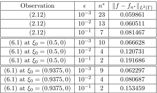
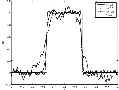
Figures 3(a)–3(c) show the comparison between the exact and numerical solutions for the timewise varying ambient temperature (6.7) of the inverse problem II with the integral observations (2.12), (6.1) with γ = 10−5,ξ0 = (0.5,0) and ξ0 = (0.9375,0), respectively, perturbed by various levels of

noiseǫ∈ {10−3,10−2,10−1}for Example 4. These levels of noise yield the stopping CGM iteration numbers n∗ _{and the L}2_{(0, T)-errors kf −f}

n∗k_L2_(0,T) given in Table 3. From this table and by

comparing Figure 3(a) with Figures 3(b) and 3(c) it can be seen that the integral observation (2.12) yields more accurate results than the point-integral observation (6.1). Also, changing the boundary point ξ0∈Γ at which a thermocouple/sensor takes the measurement (2.11) shows some

Observation ǫ n∗ _{kf −fn}∗k_L2_(Γ)

(2.12) 10−3 23 0.059861 (2.12) 10−2 _{13 0.060511}

(2.12) 10−1 7 0.081467 (6.1) atξ0= (0.5,0) 10−3 10 0.066628

(6.1) atξ0= (0.5,0) 10−2 4 0.120731

(6.1) atξ0= (0.5,0) 10−1 2 0.191686

(6.1) atξ0 = (0.9375,0) 10−3 9 0.062297

(6.1) atξ0 = (0.9375,0) 10−2 4 0.080687

(6.1) atξ0 = (0.9375,0) 10−1 2 0.153459

Table 3: The stopping CGM iteration numbers n∗ _{and the L}2_{(0, T)-errors kf −f}

n∗k_L2_(0,T) for

Example 4 of the inverse problem II with integral observation (2.12) or (6.1) perturbed by various levels of noiseǫ_{∈ {}10−3_,10−2_,10−1_}.

7

Conclusions

Multi-dimensional inverse heat conduction problems which require determining the space- or time-dependent ambient temperature appearing in the convective Robin boundary conditions of the third-kind from additional terminal, point or integral measurements have been investigated. The problems have been formulated as least-squares problems and formulae for the gradients have been delivered. A numerical method based on the CGM+BEM has been developed for obtaining a stable numerical solution when the input data is subject to noise. Numerical results for several benchmark test examples were presented in order to illustrate the feasibility of the approach. Intuitively, in the dimension > 2, the spacewise retrieval of the ambient temperature considered in the inverse problem I is more difficult than the timewise retrieval considered in the inverse problem II since we have more unknowns. But clearly, for a reliable comparison one would need to estimate the rate of decay of the singular values of the linear/affine operators involved in expressions (5.2) and (6.2) for the inverse problems I and II. This difficult task is deferred to a future work. Analogous multi-dimensional, but nonlinear inverse problems which require determining the space- and time-dependent heat transfer coefficient will be investigated in a separate future work, [6].

Acknowledgement

This research was supported by a Marie Curie International Incoming Fellowship within the 7th European Community Framework Programme and by Vietnam National Foundation for Science and Technology Development (NAFOSTED) under grant number 101.02-2011.50.

References

[1] J. V. Beck, B. Blackwell and C. R. St. Clair Jr.,Inverse Heat Conduction: Ill-Posed Problems, Wiley-Interscience, New York, 1985.

[3] Dinh Nho H`ao, A noncharacteristic Cauchy problem for linear parabolic equations II:Numer. Funct. Anal. Optim.13(5&6)(1992), 541–564.

[4] Dinh Nho H`ao, Methods for Inverse Heat Conduction Problems, Peter Lang Verlag, Frank-furt/Main, 1998.

[5] Dinh Nho H`ao, Phan Xuan Thanh, D. Lesnic, and B.T. Johansson, A boundary element method for a multi-dimensional inverse heat conduction problem,Inter. J. Computer Maths., 89(2012), 1540-1554.

[6] Dinh Nho H`ao, Phan Xuan Thanh, and D. Lesnic, Determination of the heat transfer coeffi-cients in transient heat conduction (in preparation).

[7] A. Friedman,Partial Differential Equations of Parabolic Type, Prentice-Hall, Englewood Cliffs, 1964.

[8] A.B. Kostin and A.I. Prilepko, On some problems of restoration of a boundary condition for a parabolic equation. I,Differential Equations, 32(1996), 113–122.

[9] A.B. Kostin and A.I. Prilepko, Some problems of restoring the boundary condition for a parabolic equation. II,Differential Equations, 32(1996), 1515–1525.

[10] O.A. Ladyzhenskaya, V.A. Solonnikov, and N.N. Ural’ceva,Linear and Quasilinear Equations of Parabolic Type, AMS, Providence, 1967.

[11] A. S. Nemirovskii, The regularizing properties of the adjoint gradient method in ill-posed problems. Zh. vychisl. Mat. mat. Fiz. 26(1986), 332–347. Engl. Transl. in U.S.S.R. Comput. Maths. Math. Phys., 26(2)(1986), 7–16.

[12] T.T.M. Onyango, D.B. Ingham, and D. Lesnic, Restoring boundary conditions in heat con-duction,J. Eng. Math., 62(2008), 85–101.

[13] T.T.M. Onyango, D.B. Ingham, and D. Lesnic, Inverse reconstruction of boundary condition coefficients in one-dimensional transient heat conduction, Appl. Math. Comput., 207(2009), 569–575.

[14] Phan Xuan Thanh,Boundary Element Methods for Boundary Control Problems, PhD Thesis, TU Graz, 2011.

[15] F. Tr¨oltzsch,Optimale Steuerung partieller Differentialgleichungen, Vieweg + Teubner, Wies-baden, 2005.

[16] A. Trombe, A. Suliman, and Y. Le Maoult, Use of an inverse method to determine natural convection heat transfer coefficients in unsteady state,J. Heat Transfer, 125(2003), 1017–1026.

0 0.5 1 1.5 2 2.5 3 3.5 4 0

0.5 1 1.5 2 2.5

s

f(s)

Exact

ε = 0.1

ε = 0.01

ε = 0.001

(a) Example 1

0 0.5 1 1.5 2 2.5 3 3.5 4

−0.1 0 0.1 0.2 0.3 0.4 0.5 0.6

s

f(s)

Exact

ε = 0.1

ε = 0.01

ε = 0.001

(b) Example 2

0 0.5 1 1.5 2 2.5 3 3.5 4

−0.2 0 0.2 0.4 0.6 0.8 1 1.2

s

f(s)

ε = 0.1

ε = 0.01

ε = 0.001 Exact

(c) Example 3

0 0.5 1 1.5 2 2.5 3 3.5 4 0

0.5 1 1.5 2 2.5

s

f(s)

Exact T₁ = T/3 T₁ = 2T/3 T₁ = T

(a) Example 1

0 0.5 1 1.5 2 2.5 3 3.5 4

−0.1 0 0.1 0.2 0.3 0.4 0.5 0.6

s

f(s)

Exact T1 = T/3

T1 = 2T/3

T

1 = T

(b) Example 2

0 0.5 1 1.5 2 2.5 3 3.5 4

−0.2 0 0.2 0.4 0.6 0.8 1 1.2

s

f(s)

T₁ = T/3 T

1 = 2T/3

T₁ = T Exact

(c) Example 3

Figure 2: The exact and numerical spacewise dependent ambient temperature, as a function of the arclengthsalong the boundary Γ (starting from the origin), forǫ= 10−2 and various instants

0 0.1 0.2 0.3 0.4 0.5 0.6 0.7 0.8 0.9 1 −0.2

0 0.2 0.4 0.6 0.8 1 1.2

t

f(t)

ε = 0.1 ε = 0.01 ε = 0.001 Exact

(a) Example 4 with the integral observation (2.12)

0 0.1 0.2 0.3 0.4 0.5 0.6 0.7 0.8 0.9 1

−0.2 0 0.2 0.4 0.6 0.8 1 1.2

t

f(t)

ε = 0.1 ε = 0.01 ε = 0.001 Exact

(b) Example 4 with the point-integral observation (6.1) at

ξ0 = (0.5,0) andγ= 10− 5

0 0.1 0.2 0.3 0.4 0.5 0.6 0.7 0.8 0.9 1 −0.2

0 0.2 0.4 0.6 0.8 1 1.2

t

f(t)

ε = 0.1

ε = 0.01

ε =0.001 Exact

(c) Example 4 with the point-integral observation (6.1) at

ξ0 = (0.9375,0) andγ= 10−5