A model for the reflection of shear ultrasonic waves at a thin liquid film and its application to viscometry in a journal bearing

This is a repository copy of

A model for the reflection of shear ultrasonic waves at a thin

liquid film and its application to viscometry in a journal bearing

.

White Rose Research Online URL for this paper:

http://eprints.whiterose.ac.uk/112756/

Version: Accepted Version

Article:

Schirru, M.M. and Dwyer-Joyce, R.S. orcid.org/0000-0001-8481-2708 (2015) A model for

the reflection of shear ultrasonic waves at a thin liquid film and its application to viscometry

in a journal bearing. Proceedings of the Institution of Mechanical Engineers, Part J:

Journal of Engineering Tribology, 230 (6). pp. 667-679. ISSN 1350-6501

https://doi.org/10.1177/1350650115610357

Reuse

Unless indicated otherwise, fulltext items are protected by copyright with all rights reserved. The copyright exception in section 29 of the Copyright, Designs and Patents Act 1988 allows the making of a single copy solely for the purpose of non-commercial research or private study within the limits of fair dealing. The publisher or other rights-holder may allow further reproduction and re-use of this version - refer to the White Rose Research Online record for this item. Where records identify the publisher as the copyright holder, users can verify any specific terms of use on the publisher’s website.

Takedown

If you consider content in White Rose Research Online to be in breach of UK law, please notify us by

A model for the reflection of shear ultrasonic waves at a thin liquid film 

and its application to viscometry in a journal bearing. 

Michele M. Schirru1 and Rob S. Dwyer‐Joyce1 

1

The Leonardo Centre for Tribology, The University of Sheffield, Sir Frederick Mappin Building, Mappin  Street, Sheffield, UK, S13JD 

Abstract 

The  apparent  viscosity  of  oils  in  the  thin  layers  that  exist  in  machine  elements  such  as  gears  and  bearings  is  very  different  to  that  in  the  bulk.  In  addition  oils  in  lubricating  layers  are  characterized  by  Non‐Newtonian  behaviour  due  to  the  severe  thermodynamic  conditions  that  arise.  It  is  this  viscosity  that  determines  the  film  thickness  in  lubricated  mechanical  components.  This  paper  describes  a  novel  methodology based on an ultrasonic approach to determine viscosity in‐situ in a lubricated contact. The  methodology  considers  the  lubricant  at  the  solid  boundary  as  a  Maxwell  viscoelastic  fluid  and  determines  its  response  to  an  ultrasonic  wave.  This  approach  is  then  compared  with  existing  methodologies  in  both  a  static  contact  and  in  a  rotating  journal  bearing.  The  obtained  results  have  shown that the algorithm proposed in this study is most suitable to study lubricants in the range 0.3 to 3  Pas and the measurement error has been found to be less than 10%. This viscosity range is common in  components  such  as  cam‐follower,  CVT  transmissions  and  highly  loaded  journal  bearings.  At  lower  viscosities  the  measurement  method  suffers  from  excessive  error  caused  by  the  acoustic  mismatch  between the bearing component and the oil film and the resulting difficulty in obtaining a high enough  signal to noise ratio.   

1.

Introduction 

The  ability  to  perform  real  time  and  in‐situ  monitoring  of  lubricant  viscosity  in  thin  layers  such  as  oil  films would assist in the design and testing of lubricated systems. The apparent viscosity in a thin oil film  is  different  to  that  in  the  bulk  because  fluid  particles  are  not  distributed  homogeneously  though  the  layer. The response of the fluid to a shear stress will then be different compared to that in a bulk fluid.  This  effect  is  accentuated  as  the  fluid  molecular  composition  becomes  complex.  Further,  conventional  viscometers  require  oil  to  be  extracted  once  it  has  exited  the  contact.  The  conditions  of  such  a  viscometry test can only be a simulation of the real contact parameters.  

In  this  paper  ultrasound  harmonic  waves  are  employed  as  a  suitable  technique  to  overcome  this  limitation as it is non‐invasive and can therefore be applied to the real bearing component in operation.  In ultrasonic engineering a thin layer is defined as a  “situation  where  two  successive  echoes  cannot  be  distinguished in the time domain” [1]. In that case it is not possible to measure properties such as speed  of  sound  and  fluid  impedance  by  simple  time  of  flight  measurements  [2].  Then  a  model  that  does  not  rely  on  fluid  layer  thickness  is  necessary.  Harmonic  horizontally  polarized  shear  waves  can  propagate  through  solid  layers,  but  only  minimally  into  fluid  layers  and  the  reflected  energy  from  solid‐liquid  interface is a function of the shear viscosity. Early work dedicated to the study of viscosity by means of  interaction  of  ultrasonic  shear  waves  was  performed  by  Mason  [3],  who  correlated  the  reflected  echo  wave from a torsional quartz crystal to the viscosity of a liquid layer deposited on the transducer. Since  then,  several  other  authors  have  used  reflectance  methods  to  study  viscosity  in  a  bulk  fluid  [4]  and  in  industrial  processes  where  the  fluid  involved  could  be  considered  Newtonian:  for  example  diagnostic  analysis of coal combustion processes, industrial clean up processes, and characterization of resins in an  autoclave  [5,  6].  A  number  of  studies  [7‐10]  have  taken  into  account  relaxation  effects  in  Non‐ Newtonian  lubricants  to  measure  the  rheological  parameters  involved  in  elastohydrodynamic  lubrication (EHL). These researchers explored what happens to a fluid when subjected to high pressures  and  temperature  typical  in  EHL.  Continuous  and  oscillatory  shear  were  compared  in  a  wide  range  of  frequencies, from a few kHz to hundreds of MHz. The results showed that it is necessary to incorporate  relaxation time into a model, especially under EHL conditions where normally Newtonian oils can show  Non‐Newtonian behaviour. 

The aim of this work is to determine the response of a thin oil film to shear polarized ultrasonic waves,  where  the  oil  is  modelled  as  a  generic  viscoelastic  fluid  capable  of  representing  both  Newtonian  and  Non‐Newtonian behaviour. The model is then used to determine the oil viscosity from that response to  shear ultrasound. The model is firstly validated by testing on a bench oil film and then used to measure  viscosity in‐situ and in real time in a journal bearing apparatus. 

2.

Theoretical models 

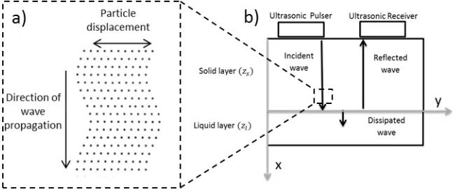
2.1 The reflection of ultrasonic shear waves from a solid‐liquid boundary 

transmitted and dissipated in the fluid, while part is reflected back to the ultrasonic source, as shown in  Figure 1 (b).  

Figure 1. a) Representation of shear wave propagation (b) Simplified model describing propagation and reflection  of an ultrasonic shear wave at solid‐liquid contact interface 

The ratio of the amplitude of the reflected wave to the amplitude if the incident wave, is known as the  reflection coefficient and can be determined by [11]: 

!!_!!!! !!

!!! !!

  (1) 

Where _!!  and _!!  are  the  acoustic  impedances  of  the  solid  layer  and  the  liquid  layer  respectively.  The  shear acoustic impedance of the solid is a real quantity defined by: 

!!! !!!  (2) 

Where !! is the density of the solid medium, and ! is the shear speed of sound in the solid. On the other  hand, the shear acoustic impedance of the liquid is a complex quantity defined by [12]: 

!!! !!!  (3) 

Where !! is the density of the fluid layer, and ! is the complex shear modulus defined as:  

! ! !!! !!!!  (4) 

Where !! is the storage modulus and !_!! is the loss modulus. As _!! is an imaginary quantity then _!!_!from  equation (1) can be written in terms of its modulus, R and phase,_!! as: 

!!_{! !!}!!∀#

     (5) 

Substituting  equation  (5)  in  equation  (1)  it  is  possible  to  obtain  a  definition  of  the  liquid  acoustic  impedance in terms of reflection coefficient modulus and phase: 

!!! !!

! ! !!! !_!�����

! ! !!!_!�����  

(6) 

2.2 Newtonian reflection model 

The  simplest  model  considers  the  liquid  as  being  Newtonian  and  the  relation  between  viscosity  and  ultrasound reflection is derived after the method of Franco et al. [13]. With reference to Figure 1, the  propagation of an ultrasonic wave at an interface is described by:  !!! ��! ! ! !!_! ��  (7) 

Where ! represents the displacement, _{! !} ! !!

 is the shear velocity where !! is the liquid density, !_! is 

the applied shear stress and x is the wave propagation direction. Here the subscript y is used to identify  shear  stresses,  where  the  particle  motion  is  normal  to  the  direction  of  propagation.  In  the  case  of  a  sinusoidal perturbation the wave equation (7) has the following solution: 

! ! !!! !∀ _!!!

!   (8) 

Where ! is the angular frequency and !! is the initial particle displacement. The Newtonian state law  correlating the shear stress !_! and strain rate ! is: 

!_{!! !!  (9)} 

Where ! is the dynamic viscosity. Combining equations (7), (8) and (9) leads to: 

 _{! !}���  (10) 

The shear modulus is defined as the stress over the strain:  ! ! !_! !  (11)  Substituting equations (10) and (11) in equation (9) gives:  ! ! ! !!     (12) 

In case of a perfectly viscous liquid the term !! from equation (4) is zero and equation (12) reduces to: 

! ! !! ! !!! !!!! ! !!!���� ! ! !!!_!����� !       (15) 

Equation  (15)  relates  viscosity  and  the  ultrasonic  reflection  coefficient  when  the  liquid  can  be  considered to be Newtonian. 

2.3 The Greenwood model 

Another  useful  equation  to  correlate  viscosity  of  a  fluid  layer  and  ultrasonic  reflection  coefficient  is  derived  by  Greenwood  [14]  starting  from  the  most  general  definition  of  acoustic  impedance  for  a  viscoelastic fluid:  !!! !_! ! ! !_! �� ��   (16)  From the definition of viscosity the shear stress is proportional to the shear strain rate and so:  !! !! ��! !!  (17)  Combining equation (17) and (7) and if equation (7) is solved with the limitation that the displacement is  sinusoidal a solution for u is obtained in the form:  ! ! !!! !∀#_!!!!!   (18) 

Where !  _{is  the  angular  frequency  and k’ is  defined  by  Greenwood  and  al.  [14]  and  it  is  solution  of} 

equation (7) only if it is equal to: 

!!_! ��

!!

!!!

!! ! !!  (19) 

Finally substituting equation (19) in equations (17) and (16) gives the definition of acoustic impedance:  

!!!

!!!!

! !! ! !! 

(20) 

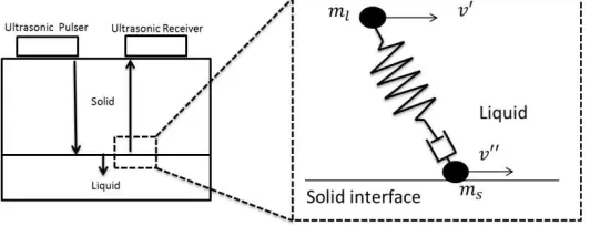
enhanced by using a Maxwell fluid analogy. This model describes, with a spring and a dashpot in series,  the interaction between solid and liquid particles excited at an interface by an ultrasonic shear wave.  

Figure 2. Maxwell analogy to describe contact interface particle interaction due to applied shear ultrasonic stress

In Figure 2 the damper element models the relaxation effects of a viscoelastic system as ultrasonic shear  occurs at the solid‐liquid boundary. The interaction between a solid particle !! and the liquid  particle 

!_{!, both subjected to ultrasonic displacements v’ and v’’, is described by a mechanical analogy. The total} 

stress and strain in the system are given by: 

!_{!! !}

! !! !! ! and  ! ! !!! !!  (22) 

Where !_!  is  the  total  stress, !  the  total  strain,  the  subscript s  refers  to  the  spring  element  while  the  subscript d to the dashpot. From Hooke law and from the dashpot theory: 

!

! !! !!! and !_{! !} ! !!!  (23) 

Differentiating equations (22) and substituting in equations (23) gives:  ! ! !!! !!! !_! ! ! !_! !  (24) 

Where k  is  the  stiffness  of  the  spring  defined  as   ! !  ,  and 

!  is  the  relaxation  time.  In  case  of  sinusoidal 

varying stress, the stress and strain are: 

!_{!! !!}!!∀# and _{! ! !!}!∀#

  (25)  Substituting equations (25) in equation (24) gives:  ! �� _!!!∀#_! ��!! ! !!! !∀#    (26)  Now by substituting equation (26) into the definition of shear modulus stated in equation (11):  ! ! ! ! ! ! ! ��� ! !���! ��!!! ! ! !!!!! ! ��� ! ! !!!! !    (27)  

Substituting the stiffness ! !!_!  into equation (27) gives: 

Separating the real and imaginary part gives:  !!_! !!�� ! ! !!!! !!! _! �� ! ! !!!!     (29)   

The system of equations (29) is a system of two equations in two unknowns, ! and !. Solving the two  equations simultaneously leads to the solution for the viscosity in case the relaxation effects are taken  into  account.  It  is  possible  to  compare  the  Maxwell  model  expressed  in  (29)  with  the  Newtonian  solutions  reported  in  section  2.2  as  follows.  Expressing  the  second  equation  of  (29)  with  respect  to !  gives: 

! !

!!! _{! ! !}!!!

!  

(30) 

The storage and loss moduli !!_and !!! _{are related to the ultrasonic reflection coefficient by equations}  (4) and (6). Combining these equations with the (30) leads to:  !! ! �� !!! !! ! ! ! !!! !   (31)  Substituting the definition of shear acoustic impedance, equation (6), into equation (31) it is possible to  directly correlate the reflection coefficient to the shear viscosity:  ! !!! ! !! !!! ! !!_!����� !! ! !!!_!�����_!! ! ! !!!! !   (32) 

It  can  be  noticed  that  equation  (32)  is  equivalent  to  equation  (14)  except  for  the  term!!!!!_{.    When} 

!!!!!_!!then equation (32) reduces to the Newtonian solution of the wave equation (14). In case of  the  Newtonian  solution  only  the  expression  (14)  exists  because  viscosity  is  a  function  of  the  loss  modulus only. 

2.5 Comparison of Models 

Figure 3. Electrical analogy to describe the incident ultrasonic wave to (a) Newtonian and (b) Viscoelastic fluids 

Figure 4 shows the amplitude of G versus frequency as the relaxation time of the lubricant is changed,  from equations (15) and (32). For low values of the relaxation time (so for!!!!!_!) the Newtonian and  the  Maxwell  models  are  identical.    For  high  values  of  the  relaxation  time  the  value G’  is  of  the  same  order as G’’ and the Newtonian model fails in describing the real oil behaviour. 

Figure 4. Comparison shear storage modulus (a) and loss modulus (b) from Newtonian and Maxwell models as  the relaxation time changes

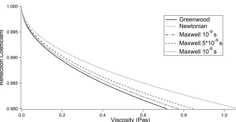
In  Figure  5  the  three  different  models  equations  (15),  (21)  and  (32)  are  compared  for  different  liquid  relaxation times. For low relaxation times the three algorithms give a similar response, while for higher  values of relaxation time only the Maxwell model is sensitive to the fluid structure changes. In all cases,  for the viscosities considered, the reflection coefficient is close to one. This is a serious limitation when  it  comes  to  practical  implementation  of  these  methods  on  a  lubricant  viscometer,  as  will  be  observed  later.  

Figure 5. Application of Newtonian and Maxwell model for different relaxation times at an aluminium‐liquid  boundary 

2.6 Application to thin films 

All these models consider the ultrasonic reflection at the boundary between a solid and liquid where the  two  bodies  are  treated  as  semi‐infinite  spaces.  The  penetration  depth  of  an  ultrasonic  shear  wave  at  MHz  frequencies  is  such  that  is  completely  attenuated  within  few  microns.  Therefore  it  is  postulated  that  the  reflection  at  a  semi‐infinite  half  space  is  equivalent  to  that  for  a  thin  oil  film,  as  shown  schematically in Figure 6. To validate this assumption the reflection coefficient was acquired from a thin  film  of  fluid  (50  micron)  and  from  a  thick  fluid  layer  (20  mm).  The  acquisition  has  been  performed  at  room temperature with three repetitions and following the experimental method reported in section 3. 

Table 1. Ultrasonic reflection coefficient and resulting calculated viscosity, from a thin liquid film compared to a  thick layer. 

Sample  Average reflection  coefficient (thin layer) 

Average reflection  coefficient (thick layer) 

Viscosity (mPas)  Thin layer 

Viscosity (mPas)  Thick layer 

S20  0.9978  0.9980  19.0  15.7 

S60  0.9946  0.9947  114.5  114.5 

S200  0.9871  0.9869  655.1  675.7 

because _!!  would  be  close  to_!!!,  from  equation  (1).  However,  at  the  current  state  of  the  art  it  is  not  convenient to implement high frequency instrumentation for engine applications due to the complexity  of the amplification system, the costs involved and because the transducers would so thin to be a fragile  quartz coating layer.     

Figure 6. Thin layer Maxwell model representation 

3. Experiments 

3.1 Apparatus 

Figure 7. Schematic diagram of the measurement apparatus  

3.2 Signal processing

The  ultrasonic  viscosity  models  depend  on  the  mechanical‐acoustic  properties  of  the  solid  and  the  density of the fluid. If these properties are known the only parameter to be determined experimentally  is the reflection coefficient. 

A five cycle sine wave from the waveform generator was used to excite the PZTs. The modulus and the  phase  of  the  reflection  coefficient  were  calculated  experimentally  by  comparing  the  ultrasonic  amplitude reflected at a solid‐liquid interface against the reference amplitude obtained by removing the  fluid sample from the upper aluminium block, and thus measuring a solid‐air contact: 

! !!! !!  

(33) 

! ! ! !_!! !! 

(34) 

Where !!  is  the  amplitude,  calculated  with  the  fast  Fourier  transform  at  the  centre  frequency  of  10  MHz,  of  the  reflected  signal  from  the  solid  liquid  interface, _!!  is  the  amplitude  of  the  reflected  signal  from  the  solid‐air  interface  (reference  measurement)  as  shown  in  Figure  8a, !_{!  the  phase  of  the} 

reflected signal from the solid liquid interface, and !

! is the phase of the reflected signal from the solid‐ air interface. As the phase is sensitive to temperature changes (±0.1 °C leads to ± 10 degrees of error)  the following relation defining the phase is obtained by manipulating equation (12) [15]: 

! ! !!!!acos_{!!! !} ! ! ! ! !

! ! !! ! 

(35) 

resonance  frequency  of  the  shear  crystal  (10  MHz)  was  considered.  The  reflection  coefficient  value  obtained  with  this  procedure  was  then  used  in  equations  (15),  (21)  and  (32)  to  obtain  oil  sample  viscosity.  

Figure 8. Example of reference and measurement signals acquired in (a) the time domain and (b) converted to the  frequency domain. 

3.3 Test lubricants 

The reflection coefficient was acquired from an aluminium‐oil interface for six different Cannon viscosity  standard calibrated lubricants (information about the test lubricants viscosities  is reported in Table 2).  The apparatus was heated up and then cooled down from 60°C down to 25 °C. Ultrasonic signals were  continuously acquired in the cooling down process and converted in reflection coefficients.  

Table 2. Cannon viscosity standard mineral oils tested 

Mineral oil  !@20°C (mPas)  !@40°C (mPas)  !@50°C (mPas) 

S20  37.32  15.27  10.65 

S60  139.1  53.83  34.69 

S200  587.4  177.5  155.8 

N350  1114  270.3  151.1 

S600  2008  446.2  240.4 

S2000  9256  1662  808.2 

4 Results and Discussion 

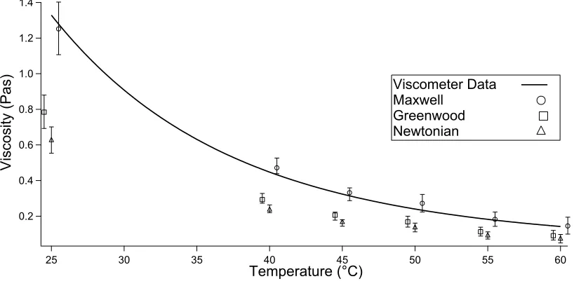
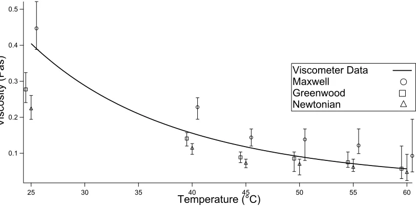
Figure  9  shows  a  set  of  the  results  obtained  for  the  oil  S600.  The  results  are  an  average  of  20  measurements executed at a given temperature range for a single fluid sample. The measured reflection  coefficient was converted to viscosity using each of the three models (equations (15), (21) and (32)) and  compared  with  the  data  expected  from  the  Cannon  oil  data  sheet.  It  is  noticeable  that  the  Maxwell  model  is  close  to  the  expected  results  at  high  viscosity,  while  the  models  give  a  similar  answer  at  low  viscosities. 

Figure 9. Variation of viscosity with temperature determined from ultrasonic reflection for a Cannon S600 mineral  oil. Three models have been used to convert reflection coefficient to viscosity, the Newtonian, Greenwood, and  Maxwell models 

Figure  10  reports  the  results  obtained  for  all  the  oils  analysed.  In  this  graph  the  line  represents  exact  agreement. It can be seen that for low viscosity lubricants the Greenwood Model results tends to be the  more effective, while as viscosity increases the Maxwell model better describes the fluid behaviour. 

1.4 1.2 1.0 0.8 0.6 0.4 0.2

Vi

sco

si

ty

(Pa

s)

60 55

50 45

40 35

30 25

Temperature (¡C)

Figure 10. Comparison of measured viscosity against expected data sheet values for all fluid samples tested. 

Using the data of Figure 10, Figure 11 shows the error between the ultrasonic measured viscosity and  the data sheet value. Three distinct regions can be identified. 

Figure 11. Error associated with each reflection model. Three regions are shown: 1) R tends to 1 and all models  are subject to scatter, (2) the optimum region for the Greenwood, (3) the optimum region for the Maxwell model 

In region 1 it is difficult to obtain accurate measurements of lubricant viscosity using any of the models.  This is because the reflection coefficient is very close to one and equations (15), (21) and (32) all become  unstable. For low viscosity lubricants and for a metal‐liquid interface the reflection coefficient modulus  is  very  close  to  the  unity  so  that  any  electrical  noise  or  disturbance  in  the  measurement  chain  has  a  significant effect on the result. For example a variation of ±1% in the reflection coefficient can lead to a  deviation of ±25mPas from the theoretical viscosity value. So for the low viscosity oil S20 the viscosity is 

100

90

80

70

60

50

40

30

20

10

Erro

r

%

8 9

0.01 2 3 4 5 6 7 8 90.1 2 3 4 5 6 7 8 9 1

Log Viscosity (Pas)

1 2 3 Maxwell model fit

5 Application to a journal bearing 

5.1 Apparatus and method 

Figure 13a and Figure 14 show the experimental journal bearing apparatus. Two ultrasonic transducers  pulsing at a centre frequency of 1.8 MHz were bonded to a brass delay line in contact with the bush, as  shown  in  Figure  13b.  A  lower  frequency  was  used  for  this  experiment  to  allow  a  better  sound  transmission  across  the  longer  solid  line.  An  electric  motor  and  pulley  system  allowed  rotation  of  the  steel  journal  shaft  between  0‐500  rpm.  The  rotational  speed  range  was  chosen  so  that  the  contact  surface  temperature  did  not  reach  a  value  such  that  the  oil  viscosity  was  too  low  to  be  within  the  sensitivity  measurement  region,  as  described  in  section  4.  The  oil  was  continuously  pumped  into  the  bearing from a reservoir thus allowing the separation of the bush and journal with a lubricating oil layer.  The  clearance  thickness  at  the  top  film  position  in  static  condition  was  100±10 _!!  [17].  This  was  measured  differentiating  the  diameter  measurements  of  the  shaft  and  the  bush  made  with  a  micrometer at different locations. The tests were run with a constant load of 200 N concentrated at the  centre  top  of  the  rig.  The  load  takes  into  account  of  the  bush  and  rig  frame  weight  plus  a  minimum  hydraulic ram load to allow proper film formation. The increment in the speed caused the lubricant to  heat  up  and  consequently  to  change  its  viscosity  throughout  the  test.  To  allow  an  accurate  measurement  of  the  oil  film  temperature  the  ultrasonic  response  from  the  first  brass  reflection  was  used because it was not possible to put a thermocouple in direct contact with the interface of interest.  

Figure 14: Journal bearing test rig

5.2 Thermal Compensation 

Figure 15. Typical amplitude vs time reflection signal acquired from the journal bearing rig.

Figure 16.  (a) Brass‐Bush ultrasonic amplitude‐ temperature calibration curve, (b) Bush‐air ultrasonic amplitude‐  temperature reference curve 

5.3 Results 

interface. The measurement signal is acquired continuously from the oil film with the shaft spinning and  every measurement has been repeated three times.  

Figure 17 shows the reflection coefficient acquired for the three different samples as the temperature  varies  due  to  shaft  rotational  speed  increase.  As  the  brass  acoustic  impedance  is  35MRayl  (approximately  double  aluminium  that  was  used  in  the  previous  case  tests),  the  reflection  coefficient  also approaches the unity for a lubricant viscosity of around 0.2 Pas. The insensitivity region (region 1 in  Figure 11) shifts from 0.01 Pas to 0.2 Pas thus eliminating the Greenwood model optimum region. For  this reason only thick oils have been tested in this apparatus.  

Figure 17. Variation of the reflection coefficient for a journal bearing oil film as the oil temperature changes due  to speed increase. 

Figure 18. Measured viscosity compared with data sheet values for three cannon standard viscosity mineral oils. 

6 Conclusions 

In  this  paper  three  models  relating  shear  ultrasonic  reflection  to  fluid  viscosity  were  implemented  for  measuring viscosity in thin lubricant layers. The models treated the fluid as Newtonian and as a Maxwell  fluid. Each model was used to process reflection results from a static captive oil film and from a rotating  journal  bearing.  In  all  cases  the  reflected  ultrasonic  signals  are  close  to  one  because  there  is  a  large  acoustic mismatch between the bearing material and the oil film. This is acerbated at low oil viscosities. 

The  Maxwell  model  has  been  developed  for  application  when  the  lubricant  is  non‐Newtonian.  It  has  been  successfully  applied  to  fluids  of  shear  viscosity  greater  than  0.15  Pas  with  resulting  accuracies  of  between 0.5% and 12% in a rotating journal bearing. The Newtonian fluid models failed (errors higher  than 100%) due to the increase in the relaxation time that invalidates the approach. This demonstrates  that it is possible to measure viscosity in‐situ in an oil film, provided the viscosity is relatively high and  that a Maxwell treatment of the fluid is applied. 

References 

1. Kinra  VK  and  Iyer  VR. Ultrasonic  measurement  of  the  thickness,  phase  velocity  and  density  or  attenuation of a thin‐viscoelastic plate. Part I: the forward problem. Ultrasonics  Vol 33 No 2 01/1995. 

3. Mason WP. Measurement of shear elasticity and viscosity of liquids at ultrasonic frequencies. Physical  Review, Volume 7S, Number 6, March I5 1949, pp 936‐946.  

4. Roth W. A New Method for Continuous Viscosity Measurement. General Theory of the Ultra‐Viscoson.  Journal of Applied Physics, vol.24, No.7, July 1953, pp 940‐950. 

5.  Sheen  SH,  Lawrence  WP,  Chien  HT  et  al. Method  for  measuring  liquid  viscosity  and  ultrasonic  viscometer. Patent No: 5,365,778, USA Nov. 22 1994. 

6. Cohen‐Tenoudji F, Ahlberg LA, Tittmann BR et al. High temperature ultrasonic viscometer. Patent No.:  4,779,452, USA Oct. 25 1988. 

7.  Barlow  AJ  and  Lamb  J. The  Visco‐elastic  behaviour  of  Lubricating  oils  under  cyclic  shearing  stress.  Proceedings  of  The  Royal  Society  A  Mathematical  Physical  and  Engineering  Sciences .  01/1959;  253(1272):52‐69.  

8. Lamb J. Physical properties of fluid lubricants: rheological and viscoelastic behaviour. Proceedings of  the Institution of Mechanical Engineers, Conference Proceedings 1967 182:293  

9.  Oldroyd  JG.  Non‐Newtonian  effects  in  steady  motion  of  some  idealised  elastic‐viscous  liquids  Proceedings  of  The  Royal  Society  A  Mathematical  Physical  and  Engineering  Sciences.  01/1958;  245(1241):278‐297. 

10. Dowson D, Higginson GR and Whitaker AV. Elasto‐hydrodynamic lubrication: a survey of isothermal  solutions. Journal of Mechanical Engineering Science June 1962 vol. 4 no. 2 121‐126   

11. Kinsler L and Frey AR. Fundamental of acoustics. Wiley, 4th edition 

12. Worlow RW. Rheological Techniques. Horwood Ltd, 1980 

13.  Franco  EE,  Adamowski  JC,  Higuti  RT  et  al. Viscosity  measurement  of  Newtonian  liquids  using  the  complex  reflection  coefficient.  IEEE  Transactions  on  Ultrasonics,  Ferroelectrics,  And  Frequency  Control,  Vol. 55, No. 10, Oct. 2008. 

14. Greenwood MS and Bamberger JA. Measurement of viscosity and shear wave velocity of a liquid or  slurry for on‐line process control. Ultrasonics 39 (2002) 623‐630.  

15.  Franco  EE,  Adamowski  JC  and  Buiochi  F. Ultrasonic  viscosity  measurement  using  the  shear  wave  reflection  coefficient  with  a  novel  signal  processing  technique.  IEEE  transactions  on  ultrasonics,  ferroelectrics, and frequency control  05/2010; 57(5):1133‐9.  

17.  Kasolang  S,  Ahmad  MA,  Dwyer‐Joyce  RS.  Measurement  of  circumferential  viscosity  profile  in  stationary journal bearing by shear ultrasonic reflection. J. Tribol. 133(3), 031501, June 17, 2011.