PriEsT: an interactive decision support tool to estimate priorities from pairwise comparison judgments

This is a repository copy of

PriEsT: an interactive decision support tool to estimate

priorities from pairwise comparison judgments

.

White Rose Research Online URL for this paper:

http://eprints.whiterose.ac.uk/102702/

Version: Accepted Version

Article:

Siraj, S orcid.org/0000-0002-7962-9930, Mikhailov, L and Keane, JA (2015) PriEsT: an

interactive decision support tool to estimate priorities from pairwise comparison judgments.

International Transactions in Operational Research, 22 (2). pp. 217-235. ISSN 0969-6016

https://doi.org/10.1111/itor.12054

© 2013 The Authors. This is the peer reviewed version of the following article: Siraj, S.,

Mikhailov, L. and Keane, J. A. (2015), PriEsT: an interactive decision support tool to

estimate priorities from pairwise comparison judgments. International Transactions in

Operational Research, 22: 217–235, which has been published in final form at

http://dx.doi.org/10.1111/itor.12054. This article may be used for non-commercial purposes

in accordance with Wiley Terms and Conditions for Self-Archiving. Uploaded in

accordance with the publisher's self-archiving policy.

[email protected]

Reuse

Unless indicated otherwise, fulltext items are protected by copyright with all rights reserved. The copyright exception in section 29 of the Copyright, Designs and Patents Act 1988 allows the making of a single copy solely for the purpose of non-commercial research or private study within the limits of fair dealing. The publisher or other rights-holder may allow further reproduction and re-use of this version - refer to the White Rose Research Online record for this item. Where records identify the publisher as the copyright holder, users can verify any specific terms of use on the publisher’s website.

Takedown

If you consider content in White Rose Research Online to be in breach of UK law, please notify us by

1. Introduction

Making decisions is a cognitive process that aims to achieve the most desired objectives with the least expected penalties. Multi-criteria Decision-Making (MCDM) refers to making decisions in the presence of several, and often conicting, criteria and objectives. The criteria in MCDM are not always supposed to be tangible, and hence may not be measurable in well-dened units. Saaty (2008) highlighted this need to measure the relative importance of given options for intangible criteria and declared the use of pairwise comparison (PC) as being central for this purpose. When n elements are to be ranked, the PC judgments can be used to construct a matrix of order n Ö n. A complete set of judgments in the PC matrix (PCM) creates an opportunity to have inconsistent information, primarily due to the redundancy inherent in its structure. The issue of inconsistency in PCs has been discussed by many authors e.g. (Ramanathan and Ramanathan, 2009; Saaty, 2008; Laininen and Hämäläinen, 2003). There exist situations in practice where the acquired judgments cannot be revised. For example, it may not be possible to revise judgments collected through anonymous surveys. Another possible reason could be to avoid cost of the revision process. In such situations, a prioritization method has to be applied in order to elicit preferences from an inconsistent set of provided judgments. Several prioritization methods have been proposed in the literature (Lin, 2007; Choo and Wedley, 2004).

The Analytic Hierarchy Process (AHP), proposed in (Saaty, 1977), is an MCDM technique based on PC to assess relative importance of criteria and alternatives. The main benet of using this approach is to convert both objective and subjective judgments into relative weights of importance. The applications of AHP have been numerous (Vaidya and Agarwal, 2006; Ngai and Chan, 2005), and it was recently considered to be the most active area of research in MCDM (Wallenius et al., 2008).

This paper presents a priority estimation tool, PriEsT, that has been developed to support AHP decision making. In contrast to existing software tools based on AHP, PriEsT better as-sists decision makers (DMs) to interactively identify and revise their inconsistent judgments based on newly proposed consistency measures. Further, PriEsT oers multiple equally-good solutions using multi-objective optimization - hence the DM has the exibility to select any of these non-dominated solutions according to his/her requirements. PriEsT is an open-source software and is freely available on the world wide web.

2. Background

The decision problems are usually decomposed into four steps i.e. dening a problem, structur-ing the problem, acquirstructur-ing judgments and nally elicitstructur-ing preferences from the acquired judgments. AHP (Saaty, 1980) is a decision making technique that enables DMs to evaluate the relative impor-tance of alternatives with the help of both, objective and subjective types of judgments. In AHP, the criteria are usually structured in a hierarchical fashion where ultimate goal is represented as root node and alternatives are placed at the bottom of this hierarchy.

Suppose, a city dweller wants to choose a mode of transporation for him to commute to the oce which is about 3 miles away from his home. He has four alternatives available in that city i.e. by bus, by car, by walk, or using a bi-cycle. The dweller - DM in this case - has to consider two main criteria of cost and convenience. Cost can be further sub-divided into one-time payments, daily charges, and maintenance cost. Similarly, the convenience criterion can also be divided into travel time, health, fatigue, and safety hazards.

After structuring the problem, the next step is to explore alternatives and acquire judgments from DM. In AHP, the judgments are acquired using the PC method where only two criteria or alternatives are compared at one time.

2.1. Pairwise Comparison Judgments

Consider a prioritization ofnelements. In the PC method, a DM assesses the relative importance of any two elements,Ei and Ej, by providing a ratio judgment aij, specifying by how muchEi is

preferred to Ej. The judgment is provided with respect to some predetermined preference scale.

In the case of tangible criteria, this can be derived from the directly measured information as, for example, weights (in kgs) or price (in euros). In the case of intangibles, a set of verbal judgments may be provided that correspond to the ratio-scale of 1 to 9 (Saaty, 1977). These judgments can be used to construct a matrixA= [aij]of the ordern×n. The PC matrix (PCM) includes all the

self-comparison and reciprocal judgments.

2.2. Inconsistency in PC Judgments

A complete set of judgments in the PC method creates an opportunity to have inconsistent information, primarily due to the redundancy inherent in its structure. There are several causes of inconsistency including psychological reasons, clerical errors and an insucient model structure (Sugden, 1985). Consistency in PCs is generally of two types i.e. cardinal consistency (CC) and ordinal consistency (OC). The judgments of DMs are cardinally consistent, ifaij =

1

aji and aij =

aikakj for alli,j and k. OC states that ifEi is preferred toEj and Ej is preferred toEk, thenEi

2.3. Measuring Inconsistency in Judgments

There exist several measures proposed to assist a DM in accepting and/or updating the acquired judgments. Widely used measures are Consistency Ratio (Saaty, 1977), Logarithmic residual mean square (Crawford and Williams, 1985) and Consistency Measure (Koczkodaj, 1993). Siraj (2011) investigated these consistency measures with the help of Monte-Carlo simulations and the results suggested a need to propose new measures for consistency. Considering the consistency test between Ei and Ej i.e. aij = aikakj (for all i, j, k), he proposed a cardinal consistency measure, called

congruence, as:

θij =

1

n−2

n

X

k=1

|log (aij)−log (aikakj)| (1)

and an ordinal consistency measure, called dissonance, as:

ψij =

1 (n−2)

X

k

step(−logaijlogaikakj) (2)

wherei6=k6=j6=iand thestep function returns 1 for positive values and 0 otherwise.

The two measures can be used together to detect and highlight outlying judgments. The congru-ence measure can also detect the prescongru-ence of consistency deadlock where all the provided judgments are equally inconsistent. It is recommended to use these measures as a useful addition to PC-based decision support tools.

2.4. Prioritization from Inconsistent PC Judgments

Suppose that there exists a preference vector r = (r1, r2, ..., r_n)T such that r_i represents the

preference intensity ofEi where i= 1,2, ..., n. However, the preference vector r is unknown to a

DM and should be estimated. The prioritization problem is to determine a priority vector w = (w1, w2, ..., w_n)T which estimates the unknown preference vectorr. The priority weights in

ratio-comparisons are considered to have non-zero positive values (wi >0) and usually calculated with

the additional constraint of normalization i.e. P

wi = 1.

There are many prioritization methods that can be applied to derive a priority vector from a set of PC judgments (Choo and Wedley, 2004). The most widely-used are the Eigenvector (EV) method (Saaty, 1977) and the Geometric Mean (GM) method (Crawford, 1987). It was shown that all prioritization methods give equal results in the case of error-free (consistent) judgments, however, the results are dierent when the PCM is inconsistent (Choo and Wedley, 2004).

Except for the EV Method, all the widely-used methods are based on optimization. In optimization-based methods, an objective function is formulated that needs to be minimized. For example, Chu et al. (1979) proposed to minimize the total deviation (TD) between the given judgments,aij and

(DLS) can be formulated as:

T D(w) =

n X i=1 n X j=1

aij −

wi

wj

2

(3)

whereP

wi = 1.

When Ei is preferred to Ej, oraij >1, it is assumed that the estimated priority vector should

preserve the preference direction i.e. wi > wj. However, while eliciting preferences, ifEj receives

a larger priority weight i.e. wi < wj, then a priority violation occurs. Considering the ratio

judgments, a violation can be formulated as a logarithmic test: vij =step

logaijlogw_wj_i

, where thestep function returns 1 for positive values and 0 otherwise.

2.4.1. Prioritization using Indirect Judgments

Mikhailov (2006) highlighted that minimizing TD produces a solution with a greater number of priority violations (NV) and therefore introduced a Two-Objective Prioritization (TOP) method to optimize both TD and NV. The use of an evolutionary multi-objective optimization technique was proposed for this purpose (Mikhailov and Knowles, 2010).

The concept of using TOP has further been developed in (Siraj et al., 2012c) which has proposed minimization of second-order deviations, TD2, along with the two objectives of TD and NV. This method of prioritization using indirect judgments (PrInT) can be formulated as:

minimize [T D(w), T D2(w), N V(w)]T

s.t. X

i

wi = 1, wi >0, i∈ {1,2, ..., n}

where

T D2(w) =

n X i=1 n X j=1 n X k=1

aikakj−

wi

wj

2

(4)

The generated priority vectors using this method are then provided to the DM to select one according to his/her requirements. Similar to TOP, the PrInT solutions can also be generated using an evolutionary multi-objective optimization approach (Mikhailov and Knowles, 2010).

These consistency measures and prioritization methods have been implemented as part of a decision aid tool called PriEsT, which is overviewed in the next section.

3. An Overview of PriEsT

new tool. PriEsT can assist DMs to interactively explore and revise their judgments based on the congruence and dissonance measures (Siraj, 2011). PriEsT also oers multiple equally-good solutions using multi-objective optimization; unlike other tools which oer only a single solution (see the companion work in (Siraj et al., 2012a)). PriEsT implements the proposed technique oering a wide range of Pareto-optimal solutions where the DM has the exibility to select any of these non-dominated solutions according to his/her requirements.

3.1. Decision Aid

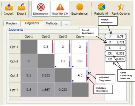
PriEsT oers dierent ways to help users identify inconsistency in their judgments. The pro-posed measure of congruence and dissonance are useful in nding the contribution of individual judgments towards overall inconsistency of a PCM and, therefore, can be used to detect and correct inconsistent judgments.

Consider the example in Fig. 1 where four alternatives are compared on the ratio scale of 1.0 to 99.0. PriEsT clearly shows the level of inconsistency for each judgment provided by a DM. The congruence and dissonance measures are plotted as bar graphs against their respective judgments. The most inconsistent triple (set of three judgments) is also shown with the help of small dots on the blamed judgments.

Other Consistency Measures Individual

Congruence

Individual Dissonance

Overall Dissonance

Overall Congruence

Figure 1: Visualizing Inconsistency in Table View

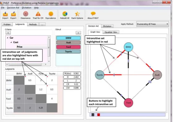
the case where there are multiple intransitive judgments, PriEsT provides the user a set of buttons below the graph view to highlight them one at a time.

Buttons to highlight each intransitive set Intransitive set highlighted in red

Intransitive set of judgments are also highlighted here with red dot on top-left

Figure 2: Graph View for Intransitive Set of Judgments

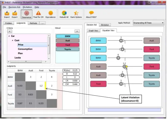
Plotting all judgments on a measurement scale has also been found useful to analyze inconsis-tency between direct and indirect judgments. This helps in visualizing cognitive dissonance present in the set of provided judgments (Siraj, 2011). Fig. 3 shows how this aids the DM in nding the potential cause of priority violations. For example, BMW has been preferred by DM over Audi, and all the other (indirect) judgments also support this order of preference. Therefore, there is no priority violation amongst these judgments. In contrast, Audi has been preferred over Ford which is in contradiction to what other judgments have suggested. This indirect judgment is highlighted as a small dot pointed by an arrow emerging from the label Latent Violation on the right side of Fig. 3.

3.2. Elicitation

Users of PriEsT are allowed to select dierent prioritization methods to estimate preferences from the same set of judgments. PriEsT therefore qualies as an appropriate research and experi-mentation tool to evaluate such methods.

3.2.1. List of Solutions and Gantt View

Latent Violation (dissonance>0)

Figure 3: Dissonance Visible in Equalizer View

3.2.2. Objective Space

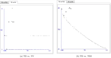
Along with TD, the need to minimize NV and TD2 has been highlighted in Section 2. PriEsT oers the DMs an interactive selection of any non-dominated solution by plotting them on two dierent objective spaces. The rst is TD-NV space as shown in Fig. 4a, while the second is TD-TD2 space, proposed in (Siraj et al., 2012a) (shown in Fig. 4b). The objective space of TD2 versus NV needs to be investigated, and will be considered for implementation in future.

PriEsT oers the DMs an interactive selection of a non-dominated solution by plotting them on a two-objective space (as proposed in (Mikhailov and Knowles, 2010)). The solutions generated by dierent methods are displayed as a list containing all numerical values of the generated weights. An alternative option is also provided for users to view the generated weights in the form of a Gantt chart.

3.3. Other features

The use of the XML format enables easy integration of PriEsT with other tools and web tech-nologies without necessitating major changes in its architecture. The use of XML also allows integration with spreadsheet applications (e.g. Microsoft Excel) and the importing of data from other software tools.

4. Rationale and Design Approach

(a) TD vs. NV (b) TD vs. TD2

Figure 4: Visualizing Solutions in Objective Space

4.1. PriEsT Engine

The core of the PriEsT software is its engine, which has been designed to be independent of user-interface libraries. The front-end has then been built on top of this engine. The engine consists of several building blocks: the base to implement basic operations and data-structures, pre-processors to remove outliers and/or estimate missing judgments, prioritization methods implementation, and analysts to calculate various properties for given problems. The building blocks are briey discussed below.

4.1.1. Base

This block consists of the basic classes required to support pairwise comparisons i.e. PC (for Pairwise Judgments), JudgmentScale (for Measurement Scales) and W (for Priority Vectors).

4.1.2. Factories

A set of factory classes generate PCMs possessing dierent properties e.g. consistent, intransi-tive, acceptable etc. In addition to this, PersistentFactory allows save and/or load of PCMs from text les (serialization).

4.1.3. Analysts

a given PCM; IndirectAnalyzer is useful to calculate θ and ψ based on indirect judgments; the TournamentAnalyzer class calculates the number of intransitive judgments (three-way cycles).

4.1.4. Pre-processors

The pre-processors cover possible pre-processing of PCMs before prioritization. For example, the CyclesRemover class suggests the removal of intransitive judgments by implementing the heuristic algorithm proposed in (Siraj et al., 2012b).

4.1.5. Methods

All prioritization methods are implemented in this block of code, including both the matrix-based and the optimization-matrix-based algorithms. Each optimization algorithm provides an objective function from the set of available objectives.

4.1.6. Objectives

This block implements the major objective functions proposed for prioritization in the PC literature. This includes TD, NV, TD2, logarithmic deviations and absolute errors. Satisfaction index is also implemented for the Fuzzy Preference Programming (FPP) method (Mikhailov, 2000).

4.2. Front-end Application

The user-interface application is based on the Model-View-Controller (MVC) architecture. Each View class has an associated Delegate class to communicate with its respective Model. All the data is ultimately preserved in a relational database. The user-interface of the PriEsT Engine was developed using the Qt framework - an open-source cross-platform software development kit (SDK) for writing applications in C++ or Java.

5. Case Study: Telecom Backbone Selection

In order to demonstrate the utility of the features of PriEsT, we consider the practical data acquired in a recent study: the selection of a backbone infrastructure for telecommunication in rural areas (Gasiea, 2010). This application is primarily focused on the rural areas of developing countries, where the lack of adequate telecommunications infrastructure remains a major obstacle for providing aordable services.

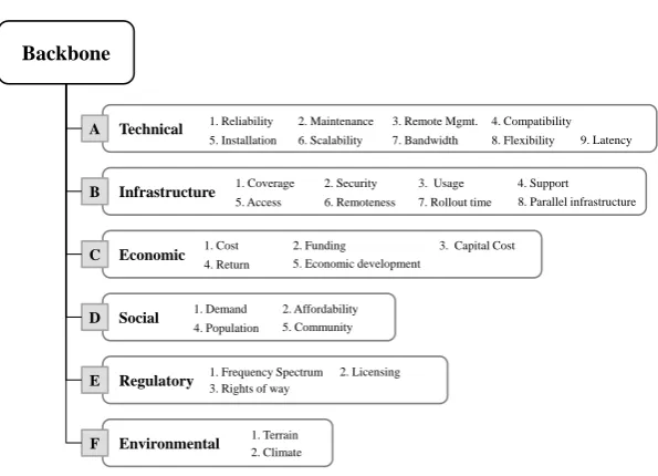
The four alternatives are Fiber-optic cable (G1), Power-line communication (G2), Microwave link (G3) and Satellite communication (G4). The problem was solved using AHP and the criteria used to compare these alternatives were grouped into six major categories including technical, infrastructural, economic, social, regulatory and environmental factors. These categories and their constituent criteria are presented in Fig. 5. The PCM, Atop, acquired for prioritizing these six

categories (top-level criteria) is shown in Fig. 6a. AlthoughAtop is a transitive PCM, the estimated

Backbone

Technical

Infrastructure

Economic

Social

Regulatory

Environmental A

B

C

D

F E

1. Reliability 2. Maintenance 3. Remote Mgmt. 5. Installation 6. Scalability 7. Bandwidth

4. Compatibility 8. Flexibility 9. Latency

1. Coverage 2. Security 3. Usage 5. Access 6. Remoteness 7. Rollout time

4. Support 8. Parallel infrastructure

1. Cost 2. Funding 3. Capital Cost 4. Return 5. Economic development

1. Demand 2. Affordability 4. Population 5. Community

1. Frequency Spectrum 3. Rights of way

2. Licensing

1. Terrain 2. Climate

Figure 5: Criteria to compare the available backbone infrastructures

The nal weights calculated using the EV and GM methods are found to be almost identical, as given in Table 1 in normalized form. Satellite communication (G4) is considered the most preferred alternative with a weight of 29.95% (using EV), followed by Microwave (G3) with a weight around 28.34% (using EV).

Optic Fiber Power-line Microwave Satellite wG1 wG2 wG3 wG4

EV: 21.7% 20.1% 28.3% 29.9%

GM: 21.7% 20.1% 28.4% 29.8%

Table 1: Estimated weights for the available backbone infrastructure options

Most criteria lie under the Technical and Infrastructure categories. The Technical category includes nine criteria whilst the Infrastructure category has eight criteria used to compare the alternatives. The two PCMs for the Technical and Infrastructure categories,Atech andAinf ra, have

been found to be intransitive and should be investigated along with Atop for their impact on the

nal result.

5.1. Investigation using PriEsT

The three matrices, Atop, Atech and Ainf ra have been analyzed using PriEsT, using both the

table-view and the graph-view. Next, we discuss these PCMs individually.

5.1.1. Atop

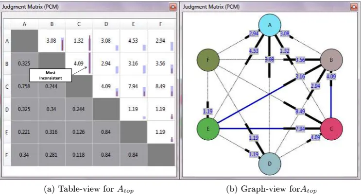
The two views forAtop are shown in Fig. 6. Fig. 6a is a snapshot of the PCM when viewed as

the labels listed in Fig. 5.

Most Inconsistent

(a) Table-view forAtop

Most Inconsistent

(b) Graph-view forAtop

Figure 6: Visualizing PC Judgments inAtop

The CR for this PCM is equal to 0.136 and therefore unacceptable in AHP terms. The con-tribution of each judgment towards overall inconsistency is visible in the table view. The most inconsistent judgment according to the congruence and dissonance measures is determined to be a23= 4.09. The graph view helps to highlight the most inconsistent set of judgments. i.e. a23,a25

anda35(see Fig. 6b). This also suggests that the judgmenta23is amongst the most inconsistent.

PCM Method w(Estimated weights) Atop

EV:

.3046 .2811 .2444 .0649 .0521 .0530 T

GM:

.3074 .2461 .2524 .0760 .0595 .0585 T

Atech

EV:

.2091 .2021 .1225 .0648 .1199 .0391 .1841 .0357 .0228 T

GM:

.2202 .1931 .1234 .0635 .1161 .0406 .1883 .0342 .0205 T

Ainf ra

EV:

.3934 .0888 .0244 .0606 .0834 .1500 .0526 .1468 T

GM:

.4102 .0821 .0246 .0530 .0928 .1398 .0555 .1420 T

Table 2: Estimated values for the criteria weights

The priority vectors obtained using EV and GM are given in Table 2. The ideal ranking possible for this PCM is A → B → C → D → E → F, however, the ranking order suggested by EV is A → B → C → D → F → E. Although the judgments were found to be transitive, the EV method has violated order of preference for one judgment i.e. the judgment a56 = 1.19 suggests

A → C → B → D → E → F. This method has also generated a priority violation but at a dierent location i.e. w2< w3 whena23>1.

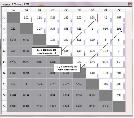
5.1.2. Atech

The table-view for Atech is shown in Fig 7. The most inconsistent judgment according to the

congruence measure is found to be a29. However, the ordinal consistency measure, dissonance,

suggestsa17 as the most inconsistent. There exists a three-way cycle in this PCM i.e. E1 →E2∼

E7→E1. The judgmenta29 does not contribute to this three-way cycle present in the PCM.

a17is ordinally the

most inconsistent

a29is cardinally the

most inconsistent

Figure 7: Table-view forAtech

EV and GM solutions are given in Table 2. Both solutions giveN V = 1.5i.e. the judgmenta17

suggests E7 →E1 whilstw1 is higher than w7 and the half-violation is added due to the presence

of preference equivalence - the judgmenta27 suggestsE2 ∼E7 but w2 is greater than w7.

An intransitive PCM cannot produce a solution with N V = 0 therefore, the three-way cycle

has to be removed. The dissonance measure suggests a17 should be revised. Therefore, inverting

the judgment of a17 will make the PCM transitive.

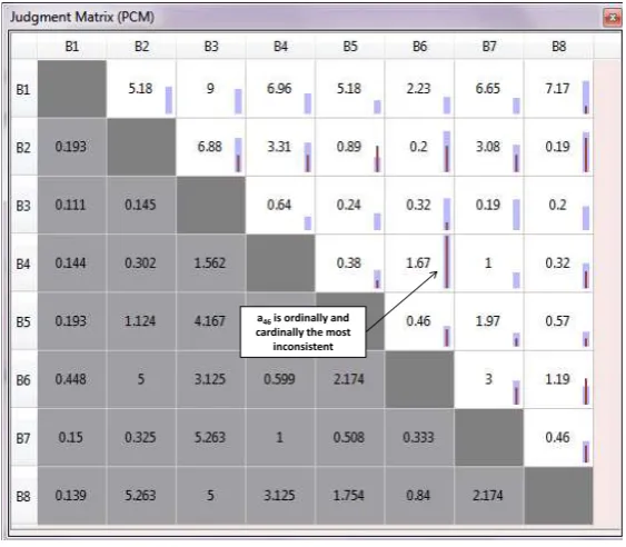
5.1.3. Ainf ra

The table-view of Ainf ra is given in Fig 8. The most inconsistent judgment according to the

congruence measure is found to bea46. The ordinal consistency measure, dissonance, also suggests

a46 as the most inconsistent. There exists four three-way cycles in this PCM i.e.

L2 : E6→E5 →E4 →E6

L3 : E4→E6 →E8 →E4

L4 : E4→E6 →E7 ∼E4

The judgment a46 = 1.666 has contributed the most to the three-way cycles present in the

PCM. By inverting only the judgmenta46, all the three-way cycles can be rectied.

The EV and GM solutions forAinf raare provided in Table 2 here both vectors generate two and

a half violations i.e. N V = 2.5. The EV solution has violated a25 while the GM solution violated

a68 instead. The judgments a46and a47 have been violated by both the EV and GM solutions.

a46is ordinally and

cardinally the most inconsistent

Figure 8: Table-view forAinf ra

5.2. Improving Consistency

Exploration of the judgment space has highlighted the main sources of inconsistency i.e., 1. Atopis found to be unacceptable in AHP terms (CR=0.136); the major source of inconsistency

is found to bea23= 4.09, which is both ordinally and cardinally most inconsistent.

2. Atech is found to be ordinally inconsistent (intransitive); inverting the judgment of a17 can

make the PCM transitive.

3. Ainf rais also an intransitive PCM withL= 4, i.e. with four three-way cycles; each three-way

cycle can be removed by inverting a single judgment i.e. a46= 1.67.

1. Atop: Change a23 from 4.09 to 0.99

2. Atech: Change a17from 0.98 to 1.01

3. Ainf ra: Change a46from 1.67 to 0.99

The suggested values are calculated using methods discussed in Siraj (2011). The nal weights calculated after these improvements are given in Table 3 in normalized form.

Optic Fiber Power-line Microwave Satellite wG1 wG2 wG3 wG4

EV: 20.7% 21.2% 29.4% 28.7%

GM: 20.8% 21.4% 29.2% 28.6%

Table 3: Weights suggested by PriEsT for the backbone infrastructure options

Satellite communication (G4) is no longer the most preferred alternative, its weight has been re-duced to 28.74% from 29.95%. The new results indicate that Microwave (G3) is the best alternative with a weight of 29.35% (using EV). The results for both EV and GM are almost in-dierentiable.

5.3. Prioritization using PrInT

As mentioned earlier, there exist situations when revision of judgments is not allowed and prioritization is required without attempting to remove inconsistency. PriEsT has the ability to solve this problem using dierent prioritization methods. The solutions for the three matrices,Atop,

Atech andAinf rahave been obtained in PriEsT using EV, GM and PrInT. The results are discussed

below.

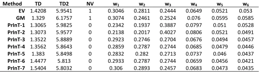
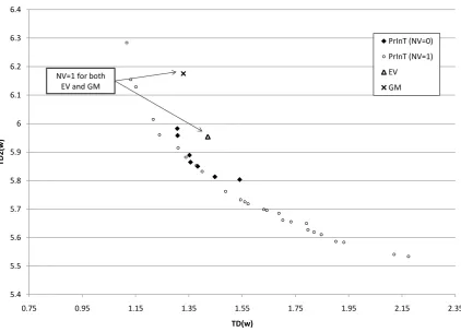
Table 4 lists the solutions forAtopgenerated by EV, GM and PrInT. When seen in the TD-TD2

plane, shown in Fig. 9, the EV and GM solutions are clearly dominated by the PrInT solutions. PrInT has produced several solutions with N V = 0 and N V = 1. Fig. 9 shows all these

solutions; the solutions havingN V >0are not listed in Table 4 being less relevant.

Method TD TD2 NV w1 w2 w3 w4 w5 w6

EV 1.4208 5.9541 1 0.3046 0.2811 0.2444 0.0649 0.0521 0.053 GM 1.329 6.1757 1 0.3074 0.2461 0.2524 0.076 0.0595 0.0585 PrInT-1 1.3065 5.9825 0 0.2342 0.1937 0.3887 0.0797 0.051 0.0528 PrInT-2 1.3073 5.9577 0 0.2138 0.2017 0.4027 0.0806 0.0521 0.0491 PrInT-3 1.3522 5.8889 0 0.2923 0.2746 0.2704 0.0676 0.0494 0.0457 PrInT-4 1.3562 5.8643 0 0.2859 0.2787 0.2744 0.0685 0.0479 0.0446 PrInT-5 1.383 5.8498 0 0.2832 0.282 0.2713 0.0737 0.046 0.0437 PrInT-6 1.4477 5.813 0 0.2933 0.2787 0.2744 0.0659 0.0456 0.0421 PrInT-7 1.5404 5.8032 0 0.306 0.2893 0.2457 0.0683 0.0473 0.0435

Table 4: Solutions forAtop

Similarly, the solutions forAtech andAinf ra are listed in Tables 5 and 6. In both cases, the EV

5.4 5.5 5.6 5.7 5.8 5.9 6 6.1 6.2 6.3 6.4

0.75 0.95 1.15 1.35 1.55 1.75 1.95 2.15 2.35

T

D

2

(w

)

TD(w)

PrInT (NV=0)

PrInT (NV=1)

EV

GM NV=1 for both

EV and GM

Figure 9: Solutions forAtopin TD-TD2 plane

The solutions generated by PrInT are equally good and therefore any of them could be selected by the DM. Consider a situation where the solutions selected are PrInT-7 for Atop, PrInT-2 for

Atech and PrInT-32 for Ainf ra (see tables 4, 5 and 6). The overall weights generated with the help

of these solutions will bewG1 = 21.3%,wG2= 19.7%,wG3 = 29.4%and wG4 = 30.6%.

Choosing a dierent solution from the set of non-dominated ones will obviously result in dierent weights. Although dierent, no solution can be declared to be inferior.

It can be argued that PriEsT should produce a single solution to support situations where user interaction is not possible. We consider this to be a future area of research: 'the selection of the most appropriate solution from within a set of Pareto-optimal solutions' in the context of pairwise comparisons.

6. Conclusion

Method TD TD2 NV w1 w2 w3 w4 w5 w6 w7 w8 w9

EV 1.3461 4.2035 1.5 0.209 0.2021 0.1225 0.0648 0.1199 0.0391 0.1841 0.0357 0.0228 GM 1.4026 4.0775 1.5 0.2202 0.1931 0.1234 0.0635 0.1161 0.0406 0.1883 0.0342 0.0205 PrInT-1 1.3383 4.1109 0.5 0.1973 0.1652 0.147 0.0613 0.1453 0.0366 0.1994 0.0274 0.0204 PrInT-2 1.3803 4.0947 0.5 0.1956 0.1691 0.1461 0.0636 0.1316 0.0357 0.209 0.0291 0.0202 PrInT-3 1.4025 4.0309 0.5 0.1962 0.1841 0.1333 0.0673 0.1331 0.0353 0.2016 0.0293 0.0198 PrInT-4 1.4289 4.0119 0.5 0.1945 0.1791 0.1392 0.0621 0.1353 0.0401 0.2014 0.0294 0.0191 PrInT-5 1.4448 4.0111 0.5 0.1973 0.1775 0.138 0.0615 0.1341 0.0439 0.1996 0.0291 0.0189

Table 5: Solutions forAtech

and highlights intransitive set of judgments present in a given PCM. In the case of inconsistent judgments, PriEsT oers a wide range of Pareto-optimal solutions based on multi-objective op-timization. The DM has the exibility to select any of these non-dominated solutions according to his/her requirements. So far, PriEsT has been developed as a prototype; the future aim is to develop PriEsT in accordance with international standard ISO/IEC 9126.

The features of PriEsT have been demonstrated and evaluated through its application to a real-world case study: the selection of the most appropriate Telecom infrastructure for rural areas. This use of PriEsT has highlighted the presence of intransitive judgments in the acquired data and the correction of these judgments has led to a dierent ranking of the available alternatives.

References

Choo, E. and Wedley, W. C. (2004). A common framework for deriving preference values from pairwise comparison matrices. Computers & Operations Research, 31(6):893908.

Chu, A., Kalaba, R., and Spingarn, K. (1979). A comparison of two methods for determining the weights of belonging to fuzzy sets. Journal of Optimization Theory and Applications, 27(4):531538.

Crawford, G. B. (1987). The geometric mean procedure for estimating the scale of a judgement matrix. Mathematical Modelling, 9(3-5):327334.

Crawford, G. B. and Williams, C. (1985). A note on the analysis of subjective judgment matrices. Journal of Mathematical Psychology, 29(4):387405.

Forman, E., Saaty, T., Selly, M., and Waldron, R. (1983). Expert Choice. Decision Support Software, McLean, VA. Gasiea, Y. (2010). An Analytic Decision Approach to Rural Telecommunication Infrastructure Selection. PhD thesis,

Manchester School of Mechanical, Aerospace and Civil Engineering, University of Manchester.

Hämäläinen, R. P. and Lauri, H. (1995). HIPRE 3+ User's Guide. Systems Analysis Laboratory, Helsinki University of Technology.

Koczkodaj, W. (1993). A new denition of consistency of pairwise comparisons. Mathematical and Computer Modelling, 18(7):7984.

Laininen, P. and Hämäläinen, R. P. (2003). Analyzing ahp-matrices by regression. European Journal of Operational Research, 148(3):514524.

Lin, C. (2007). A revised framework for deriving preference values from pairwise comparison matrices. European Journal of Operational Research, 176(2):11451150.

3.6 3.7 3.8 3.9 4 4.1 4.2 4.3 4.4

0.75 0.95 1.15 1.35 1.55 1.75 1.95 2.15 2.35

T

D

2

(w

)

TD(w)

PrInT (NV=0.5)

PrInT (NV=1.5)

EV

GM

NV=1.5 for both EV and GM

Figure 10: Solutions forAtechin TD-TD2 plane

Mikhailov, L. (2006). Multiobjective prioritisation in the analytic hierarchy process using evolutionary computing. In Tiwari, A., Knowles, J., Avineri, E., Dahal, K., and Roy, R., editors, Applications of Soft Computing: Recent Trends, pages 123132. Springer.

Mikhailov, L. and Knowles, J. (2010). Priority elicitation in the ahp by a pareto envelope-based selection algorithm. In Ehrgott, M., Naujoks, B., Stewart, T., and Wallenius, J., editors, Multiple Criteria Decision Making for Sustainable Energy and Transportation Systems, volume 36, pages 249257. Springer.

Ngai, E. and Chan, E. (2005). Evaluation of knowledge management tools using AHP. Expert Systems with Appli-cations, 29(4):889 899.

Ramanathan, R. and Ramanathan, U. (2009). A qualitative perspective to deriving weights from pairwise comparison matrices. Omega, 38(3-4):228232.

Saaty, T. L. (1977). A scaling method for priorities in hierarchical structures. Journal of Mathematical Psychology, 15(3):234281.

Saaty, T. L. (1980). The Analytic Hierarchy Process, Planning, Piority Setting, Resource Allocation. McGraw-Hill, New York.

Saaty, T. L. (2008). Relative measurement and its generalization in decision making. why pairwise comparisons are central in mathematics for the measurement of intangible factors - the analytic Hierarchy/Network process. Real Academia de Ciencias, España, 102(2):251318.

Siraj, S. (2011). Preference Elicitation from Pairwise Comparisons in Multi-criteria Decision Making. PhD, The University of Manchester, Manchester, UK.

5.2 5.4 5.6 5.8 6 6.2 6.4 6.6

1.2 1.4 1.6 1.8 2 2.2 2.4 2.6 2.8 3

T

D

2

(w

)

TD(w)

PrInT (NV=1.5)

PrInT (NV=2.5)

EV

GM

NV=2.5 for both EV and GM

Figure 11: Solutions forAinf rain TD-TD2 plane

& Operations Research, 39(2):191 199.

Siraj, S., Mikhailov, L., and Keane, J. (2012b). A heuristic method to rectify intransitive judgments in pairwise comparison matrices. European Journal of Operational Research, 216(2):420 428.

Siraj, S., Mikhailov, L., and Keane, J. A. (2012c). Preference elicitation from inconsistent judgments using multi-objective optimization. European Journal of Operational Research, 220(2012):461471.

Sugden, R. (1985). Why be consistent? a critical analysis of consistency requirements in choice theory. Economica, 52(206):167183.

Vaidya, O. and Agarwal, S. (2006). Analytic hierarchy process: An overview of applications. European Journal of Operational Research, 169(1):129.

Method TD TD2 NV w1 w2 w3 w4 w5 w6 w7 w8

EV1.5716 5.8996 2.5 0.3934 0.0888 0.0244 0.0606 0.0834 0.15 0.0526 0.1468 GM1.5875 5.8581 2.5 0.4102 0.0821 0.0246 0.053 0.0928 0.1398 0.0555 0.142 PrInT-1 1.3041 6.3398 1.5 0.3768 0.0919 0.0339 0.051 0.0923 0.1639 0.0544 0.1358 PrInT-2 1.3089 6.2998 1.5 0.3884 0.0761 0.0339 0.0511 0.0876 0.1637 0.0613 0.1379 PrInT-3 1.3188 6.2426 1.5 0.3851 0.0822 0.0317 0.0509 0.0918 0.163 0.0612 0.134 PrInT-4 1.334 6.1952 1.5 0.3657 0.0855 0.0309 0.0474 0.0996 0.1712 0.0513 0.1484 PrInT-5 1.3468 6.1379 1.5 0.3712 0.0712 0.0306 0.0465 0.093 0.1663 0.0553 0.1659 PrInT-6 1.354 6.1332 1.5 0.3886 0.0766 0.0313 0.0482 0.0855 0.1609 0.052 0.157 PrInT-7 1.386 6.05 1.5 0.3739 0.0809 0.0285 0.0462 0.0893 0.1641 0.0542 0.163 PrInT-8 1.4015 6.0309 1.5 0.3627 0.0738 0.0279 0.0434 0.0946 0.1707 0.0568 0.1701 PrInT-9 1.4092 6.0227 1.5 0.3622 0.0732 0.0277 0.0421 0.1002 0.1706 0.0567 0.1673 PrInT-10 1.427 5.9753 1.5 0.3739 0.0717 0.0274 0.0449 0.0926 0.1672 0.0556 0.1668 PrInT-11 1.4376 5.958 1.5 0.3768 0.0714 0.0272 0.0447 0.0922 0.1665 0.0552 0.1659 PrInT-12 1.4574 5.942 1.5 0.394 0.076 0.027 0.0479 0.0847 0.1589 0.0557 0.1558 PrInT-13 1.4853 5.8961 1.5 0.3852 0.061 0.027 0.0484 0.0856 0.1716 0.0523 0.1689 PrInT-14 1.4925 5.8848 1.5 0.3814 0.0607 0.0268 0.044 0.0993 0.1713 0.052 0.1646 PrInT-15 1.5187 5.8578 1.5 0.3933 0.0602 0.0272 0.0429 0.0848 0.1728 0.0524 0.1665 PrInT-16 1.5421 5.8442 1.5 0.3651 0.0587 0.0262 0.0427 0.0824 0.1917 0.0507 0.1826 PrInT-17 1.563 5.8152 1.5 0.3884 0.0605 0.0267 0.0408 0.0881 0.1822 0.0478 0.1654 PrInT-18 1.6307 5.7461 1.5 0.3785 0.0595 0.024 0.0427 0.0874 0.183 0.0574 0.1676 PrInT-19 1.6404 5.7275 1.5 0.3803 0.0594 0.0242 0.0429 0.0881 0.1839 0.0526 0.1685 PrInT-20 1.6546 5.7216 1.5 0.3793 0.053 0.0244 0.0429 0.0881 0.1837 0.0523 0.1763 PrInT-21 1.6912 5.6845 1.5 0.3946 0.0615 0.0239 0.0431 0.0854 0.1776 0.0507 0.1632 PrInT-22 1.7043 5.6739 1.5 0.3894 0.0567 0.0239 0.042 0.0862 0.1782 0.0512 0.1725 PrInT-23 1.7194 5.6612 1.5 0.3842 0.064 0.0233 0.0427 0.0877 0.1824 0.0477 0.168 PrInT-24 1.7415 5.645 1.5 0.3825 0.0631 0.0229 0.0426 0.0864 0.1801 0.0497 0.1729 PrInT-25 1.7554 5.6372 1.5 0.3788 0.0632 0.0229 0.0421 0.0865 0.1804 0.0465 0.1794 PrInT-26 1.7938 5.6113 1.5 0.396 0.0575 0.0227 0.0444 0.0856 0.1793 0.0509 0.1636 PrInT-27 1.8223 5.5886 1.5 0.3919 0.0625 0.0225 0.0416 0.0855 0.1783 0.0462 0.1714 PrInT-28 1.8455 5.5736 1.5 0.3897 0.0547 0.0223 0.0437 0.0842 0.1826 0.0485 0.1745 PrInT-29 1.8842 5.5492 1.5 0.3868 0.0529 0.022 0.0428 0.0884 0.1843 0.0472 0.1757 PrInT-30 1.9217 5.5288 1.5 0.383 0.057 0.0212 0.0427 0.0868 0.1834 0.0484 0.1775 PrInT-31 1.9579 5.5079 1.5 0.3994 0.0579 0.0215 0.0416 0.0879 0.1783 0.0458 0.1675 PrInT-32 1.9931 5.4913 1.5 0.4028 0.0518 0.0215 0.042 0.0862 0.1807 0.0462 0.1689 PrInT-33 2.0467 5.4605 1.5 0.3867 0.0519 0.0209 0.0405 0.0833 0.2007 0.0449 0.1712 PrInT-34 2.0827 5.4536 1.5 0.376 0.0504 0.0202 0.0394 0.081 0.1951 0.049 0.1888 PrInT-35 2.1712 5.4026 1.5 0.3862 0.0528 0.0198 0.0392 0.0882 0.1935 0.043 0.1773 PrInT-36 2.2311 5.3844 1.5 0.3961 0.0525 0.0195 0.0423 0.0778 0.1922 0.0442 0.1754 PrInT-37 2.2893 5.3603 1.5 0.3822 0.0555 0.0189 0.0377 0.0847 0.2029 0.0434 0.1747 PrInT-38 2.3217 5.3511 1.5 0.3798 0.0545 0.0187 0.0374 0.0842 0.2086 0.0431 0.1736 PrInT-39 2.3708 5.331 1.5 0.3897 0.0506 0.0188 0.037 0.0842 0.2015 0.0422 0.176 PrInT-40 2.4036 5.3214 1.5 0.3919 0.0502 0.0187 0.0368 0.0839 0.2002 0.0419 0.1763 PrInT-41 2.418 5.3173 1.5 0.3922 0.0504 0.0186 0.0373 0.0839 0.2007 0.0419 0.175 PrInT-42 2.4985 5.2996 1.5 0.3869 0.0507 0.0179 0.0371 0.0847 0.1951 0.0422 0.1855 PrInT-43 2.524 5.2925 1.5 0.3958 0.0507 0.0179 0.0371 0.0847 0.1958 0.0423 0.1755 PrInT-44 2.5748 5.2811 1.5 0.3894 0.0499 0.0176 0.0365 0.0834 0.1989 0.0416 0.1827 PrInT-45 2.6626 5.2694 1.5 0.3842 0.0505 0.0171 0.0344 0.0845 0.2018 0.0421 0.1855 PrInT-46 2.6936 5.2629 1.5 0.3976 0.0503 0.0173 0.0349 0.0851 0.2033 0.0408 0.1706 PrInT-47 2.756 5.2547 1.5 0.392 0.0506 0.0169 0.034 0.0835 0.1996 0.0398 0.1835 PrInT-48 2.8598 5.246 1.5 0.3797 0.0481 0.0165 0.0335 0.0813 0.2235 0.039 0.1785