Cooling system analysis for a data center using liquid immersed servers

This is a repository copy of

Cooling system analysis for a data center using liquid

immersed servers

.

White Rose Research Online URL for this paper:

http://eprints.whiterose.ac.uk/89709/

Version: Accepted Version

Article:

Almaneea, A, Thompson, HM, Summers, JL et al. (1 more author) (2014) Cooling system

analysis for a data center using liquid immersed servers. International Journal of Thermal

Technologies, 4 (3). pp. 200-207.

[email protected] https://eprints.whiterose.ac.uk/ Reuse

Unless indicated otherwise, fulltext items are protected by copyright with all rights reserved. The copyright exception in section 29 of the Copyright, Designs and Patents Act 1988 allows the making of a single copy solely for the purpose of non-commercial research or private study within the limits of fair dealing. The publisher or other rights-holder may allow further reproduction and re-use of this version - refer to the White Rose Research Online record for this item. Where records identify the publisher as the copyright holder, users can verify any specific terms of use on the publisher’s website.

Takedown

If you consider content in White Rose Research Online to be in breach of UK law, please notify us by



Abstract—data centers are large consumers of power, of which a large proportion is spent on removing the heat generated by the semiconductors inside IT servers. This paper develops a full analysis of the cooling system when servers are immersed in a dielectric liquid and water is used to transport the heat outside of the data center. The analysis combines empirical curve fits and flow analysis with computational fluid dynamics (CFD) simulations of liquid immersed servers placed in parallel in a rack of a data center. The liquid immersed server concept is based on a dielectric liquid that is in direct contact with the semiconductor components to improve heat rejection. The heat generated from the microelectronics is naturally convected, via buoyancy, in the dielectric liquid to a cold plate on the opposing side. The cooling system of the data center in this study consists of a dry air cooler and a liquid-to-liquid buffer heat exchanger. It was found that the power usage effectiveness (PUE) is as low as 1.08 for the cooling system. The results also show that the PUE is affected by the server-rack occupancy and can increase by 26% as occupancy drops by 80%, thus the better the server-rack occupancy, the better the PUE.

Keywords— data center, liquid cooling, power usage effectiveness, liquid immersed servers.

I. INTRODUCTION

he increasing demand for digital services today has led to an unprecedented growth globally in data centers and their energy demand. Efficient cooling of data center is needed, since over 30 % of data center power consumption is used for cooling [1, 2]. Data centers can be cooled by the more traditional air cooling, but some are now being cooled directly with the aid of liquids [3]. The latter approach is usually used in data centers with high density racks. The liquid cooling of data centers can be classified in essentially three ways; rack heat exchanger, in server and on chip heat exchangers and total liquid immersion. The heat transfer in the immersed server is by way of natural convection of a dielectric liquid, which transfers the thermal energy produced by the microelectronics into a water jacket, through which a pumped coolant passes[4, 5].

The main interest in this paper involves the integration of liquid immersed servers in the whole data center cooling system. The cooling system in this study consists of dry air cooler and buffer heat exchanger, together they can reject the

A. Almaneea, H. Thompson, J. Summers and N. Kapur are with Institute of Engineering Thermofluids (iTF), School of Mechanical Engineering, University of Leeds, United Kingdom (corresponding author: Mechanical Engineering, University of Leeds, LS2 9JT, Leeds, UK, email: [email protected]).

heat from racks via liquid loops. The cooling system is explained in detail in the next sections. The ambient temperature for the calculations in this paper are taken for the city of Leeds [6]. A MATLAB program is used to calculate the inlet water temperature to the rack based on the ambient temperature and pump flow rates. With the evaluated rack inlet flow rate and temperature, a computational model based on COMSOL is used to determine the outlet temperature and pressure drop for the immersed servers. The power of the pumps can be determined for the pressure drop and flow rate. The power usage effectiveness (PUE) of the data center is calculated from the IT power consumption and power consumed by the pumps and fans in the cooling loop. The variation of PUE is determined with varying rack load and is also presented.

II.COOLING DATA CENTER SYSTEM

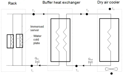
A schematic diagram of the data centre cooling system that is used in this section is shown in Fig.1. On the right of the figure is a dry air cooler and fan, which moves the air at the ambient outside temperature (T5) through the heat exchanger.

A pump circulates the water from the dry air cooler heat exchanger to a buffer (liquid-to-liquid) heat exchanger at a flow rate, Qinr, to reject the heat from the data center. On the

left side of the figure the immersed servers are housed in the rack and are connected to the buffer heat exchanger via a liquid loop inside the data center. A second pump circulates water between the buffer heat exchanger and the racks at a flow rate, Qins. The cold (supply) temperature to the buffer

heat exchanger is T3 and the inlet (supply) water temperature

to the servers is, T1.

Fig. 1 Schematic diagram of the data center cooling system

Cooling system analysis for a data center using

liquid immersed servers

A. Almaneea, H. Thompson, J. Summers and N. Kapur

The model using COMSOL is applied to simulate the heat transfer at the server level only. However, the data of dry cooler and buffer heat exchanger data are taken from an experimental study [7]. They studied a data center cooling system experimentally, which had a cooling system arrangement that included a dry cooler, buffer heat exchanger and servers that were cooled by a combination of pumped water cold plates on the CPU and air, via fans, for the rest of the server.

In this study, the server is fully immersed without any air used to cool the servers. Therefore, the relative humidity is not considered in the system. This gives an advantage of limiting the number of variables to be only the temperature. The ambient temperature, T5, is chosen for the city of Leeds,

England [6]. The annual average temperature of Leeds is shown in Fig. 2.

Fig. 2 Average temperature of Leeds, England [6]

III. METHODOLOGY OF FLOW RATE AND TEMPERATURE CALCULATION

In the previous section, the data center cooling system and method of obtaining the ambient temperature, T5, were

explained. This section develops an approach to determine the other system parameters, which are the flow rate from dry cooler to buffer heat exchange, Qinr, the flow rate from the

buffer heat exchanger to the rack, Qins, the cold (supply) water

temperature entering the buffer heat exchanger, T3, and the

water inlet temperature of server, T1.

The values of the flow rates, Qins and Qinr are 5, 7.5, 10

GPM, which are taken from experimental work [7] as explained in section II. In [8], a graph is plotted between ∆Tapr

and the flow rate, Qinr, for dry cooler fan speeds of 169 rpm. The ∆Tapr is the temperature difference between the ambient

temperature, T5, and the inlet water temperature of buffer heat

exchanger, T3. The flow rate, Qins, and dry air cooler fan speed

used are taken directly from [7], however the cooling load is different. In [7] the ∆Tapr is varied with Qinr has been plotted at

a cooling load of 15,000 W, where the rack cooling load in this work is 5000 W (each server load is 100 W and the number of servers in one rack is 50 servers). As the flow rate and fan speed are the same as used in [8] and the heat load is different, the ∆Tapr is scaled down by interpolating between

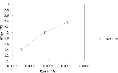
two rack heat load, 5KW and 15KW. Fig. 3 shows the

variation of ∆Tapr at different flow rates, Qinr, where the fan of

dry cooler is spinning at 196 rpm and a cooling load of 5000 W.

Fig 3. The variation of ∆Tapr with flow rate Qinr, dry cooler fan

spins at 169 rpm.

The flow rate, Qinr, is function of ∆Tapr and this function is

obtained from curve fitting the graph in Figure 3, it is expressed as:

The flow rate between the dry cooler and the buffer heat exchanger, Qinr, is known, so the ∆Tapr can be calculated from

the equation above and the inlet water temperature to the buffer heat exchanger, T3, can be evaluated using

Having obtained the value of T3, the next step is to

determine the inlet water temperature to the servers, T1. The

value of T1 is based on ∆Taps, which is the temperature

difference between the water temperature entering the buffer heat exchanger, T3, and the inlet water temperature to the rack,

T1, based on the following relationship

The value of ∆Taps is conducted from Qins and Qinr. The

values of Qins and Qinr are varying at 5, 7.5 and 10 GPM. In [7] the graph lines for ∆Taps varying with Qins and Qinr which is

done at cooling load 15,000 W . In this section the rack cooling load is 5000 W and the flow rate is kept the same as in the experimental work, [7], however the cooling load is different so ∆Taps is scaled down as explained before. Fig. 4

shows the variation of ∆Taps for a 5000 W cooling load for

Fig 4. The variation of ∆Taps with Qins and Qinr

The ∆Taps is affected by the Qins and the Qinr variation and

the relation can be obtained by fitting curves from the results in Fig.4. The equations of ∆Taps can be expressed as:

At Qins = 5 GPM

At Qins = 7.5 GPM

At Qins = 10 GPM

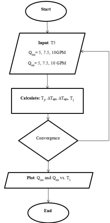
The M script in MATLAB v7.11 is used to solve all above equations to find the inlet water temperature of the rack, T1.

The flow chart of the programing steps is shown in Fig. 5.

IV. RESULTS OF RACK INLET TEMPERATURE

This section presents the results of the rack water inlet temperature, T1, which is obtained from MATLAB. The

ambient temperature that is selected from Fig. 2 is T5 = 19 o

C which is the highest temperature of the year in Leeds [6]. There are two flow rates through the buffer heat exchanger the first one is the flow rate from dry air cooler heat exchanger to buffer heat exchanger, Qinr, and the second flow rate is from

the buffer heat exchanger to the rack, Qins. The flow rates, Qins

and Qinr, are set independently to a value from 5, 7.5 and 10

GPM.

The effects of varyingthe flow rates on the rack water inlet temperature, T1, are presented in Fig. 6. Both flow rates, Qins

and Qinr, are varied independently between the values 5, 7.5

and 10 GPM. The results show that T1 decreases with

increasing Qinr and decreasing Qins. The lowest T1 value is

found to occur, at the highest Qinr and lowest Qins.

Fig 5. Flow chart of calculations to find T1 using MATLAB

v7.11.

Fig 6. : Water inlet temperature of rack, T1, varying Qinr for

different Qins.

V.SIMULATION MODEL AND RESULTS

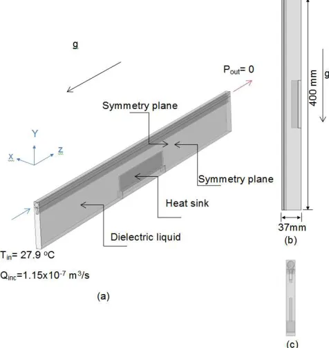
The geometry and boundary condition of the liquid immersed server model is shown in Fig. 7. Heat is generated from the CPU underneath the heat sink and cooled by the water that passes through the cooler solid block representing the water jacket at T1= 27.9 oC and Qins= 5 GPM. The

conjugate heat model with symmetry planes for the immersed server is simulated via COMSOL 4.3. The simulation model set up is validated against the experimental work of natural heat convection in [9], where a 320mm x 200mm x 40mm enclosure with fins attached on the hot wall. The buoyancy drives the flow inside the enclosure due to the temperature difference between the hot and cold walls. The average error between the simulation model presented here and the experimental work is 4.8%.

Fig 7. The geometry of the symmetry simulation model used in COMSOL a) Isometric view b) Side view c) Front View

In this study, the model consists of two types of fluid flow. The dielectric liquid is circulating inside the server due to natural convection and the other fluid is flowing by forced convection through the channel. Before solving the full conjugate heat model, the two fluid flows are checked to determine whether the flow is turbulent. For the water flowing in the channel this is determined by calculating the Reynolds number, Re

Where D is the water channel diameter (3.5x10-3 m), V is the average flow velocity (1.2x10-2m/s), w (996.6 kg/m3) and

w (7.96x10-4 pa.s) are the density and viscosity of water,

respectively. The Re is 53 for a flow rate of 1.15x10-7 m3/s and

can therefore be considered as laminar [10].

For natural convection inside the server, the dielectric fluid flow behaviour can be indicated by using Rayleigh number [11], Ra

Where H is the server height, q is the heat flux per unit area, g is the acceleration of gravity, cpis Specific heat capacity, D is density, Dis the thermal conductivity, Dis viscosity, is

the coefficient of volumetric expansion. All these fluid thermal properties are taken from Chi et al [12] and listed in Table 1. The Ra is equal to 1.8x108, which is greater than 107 and indicates therefore that the flow is turbulent [13].

Inside the server the fluid flow is turbulent and governed by the conservation equations for mass, momentum and energy for turbulent natural convection of the dielectric liquid domain,

Continuity equation

Momentum equation p

k

The body force is F which mainly depends on the density variation. The temperature increases the density of the fluid decreases. This driving buoyancy force which can be expressed as:

T

Where g = (0, 0, ).

The dielectric fluid has density-temperature variations

(T) = 1716.2 -2.2T

In turbulent natural convection in enclosures, the k-turbulent model has been found to be a robust model which can offer solutions close to experimental results as investigated in [14-16]. The k- turbulent models introduce two additional variables turbulent kinetic energy, k, and

specific dissipation rate, . The transport equations are based on [17], which are applied in the CFD model are:

k

k

p

p

The turbulent viscosity can be defined as

DT

The production term is found from the fluid velocity as

p

Energy equation

c

T

c

T

Where D is thermal conductivity and PrT is turbulent

Prandtl Number (using Kays-Crawford)

The empirical turbulent model constants parameters are

For the water channel which is the forced convection laminar fluid domain, the governing equations are:

Continuity equation

Momentum equation

p

Energy equation

c

T

T

In the solid domain, only the energy equation is required

T

Where, the s is the thermal conductivity for the solids

which are Copper and Aluminum.

The material of the heat sink is copper and the baffles and cold plate are made of Aluminium alloy. The working fluids in this paper are water and a dielectric liquid (see Error!

Reference source not found. 1 for properties). The water is

used as cooling liquid that passes through the cold plate channel and the server is filled with the dielectric liquid for which the thermal properties are kept constant except for the density which is a function of temperature.

TABLE1

THERMAL PROPERTIES OF DIELECTRIC LIQUID

Properties Abbrev. Dielectric Fluid

Specific heat capacity CpD 1140 (J/kg.K)

Thermal expansion D 1.151496x10

-3

(K-1 )

Dynamic viscosity µD 1.124782x10-3 (Pa.s)

Thermal conductivity D 6.9x10-2 (W/m.K)

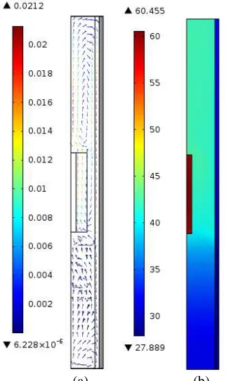
A typical fluid flow inside the immersed server is shown in fig.8 (a). The heat transferred to the liquid as it flows through the CPU heat sink leads to a buoyancy-driven flow which results in the liquid rising on the left hand portion above the CPU and falling on the right side as it is cooled by the cold plate. The flow velocities below the CPU are generally smaller than those above it. The corresponding temperature field is shown in fig 8(b) and demonstrates that the liquid above the CPU is significantly hotter than that below it. The CFD analysis is very important in practice as it enables the maximum temperature of the CPU, Tcase, which must be

constrained to ensure its reliable operation, to be predicted. In the example below Tcase=60.4oC.

(a) (b) Fig 8. a) Velocity field inside the server for the dialectic liquid. b) Temperature filed

The simulation model based on COMSOL 4.3b is now used to determine the rack outlet temperature, T2, and pressure drop

in order to calculate the required pump power.

The water inlet temperature of the server channel is Tin=

T1= 27.9 oC. The flow rate of the rack is Qins = 5 GPM and the

flow rate used in the server cold plate water channel is: Flow rate for one water channel

F R R GPM N O Sx N O C S

x x

Where F.R.R is flow rate to the rack, N.O.S is number of servers per rack and N.O.C.S is the number of water channels in one server.

The pressure drop across the water channel (∆Pch) is found

be 11.6 Pa of the simulation model with temperature inlet to the server water channel equal to 27.9 oC and the water flow rate inlet server channel is 1.15x10-7 m3/s.

VI. PUEOFCOOLINGSYSTEM

The power usage effectiveness (PUE) is used to indicate the effectiveness of the data center cooling systems and is

efficiency [18]. The equation that is used to calculate the PUE is [19, 20]

The power of data center utilities and power of IT is required to calculate the PUE. The power consumed by the IT in this work is coming from the rack power which is

PIT = 50x100W= 5.0 kW

In this study there are two pumps to circulate water between the heat exchangers and fans to reject heat from the dry air cooler. The power of the pump, Pps, that circulates the water

between the rack and buffer heat exchanger is determined by [21]

Where, Qins is flow rate between the rack and buffer heat

exchanger, is the pump efficiency. The pressure drop from the simulation model for one channel is ∆Pch =11.6 Pa

The pressure drop for the rack is given by,

∆Ps= N.O.S x N.O.C.S x ∆Pch =50x55x11.6 = 31.9 kPa

Pump efficiencies are between 0.5 and 0.6 [22], in this study the pump efficiency is chosen to be 0.5 for the worst case scenario. The power required pumping the water between the rack and buffer heat exchanger is

The power required by the dry air cooler heat exchanger fans is based on the flow rate and pressure drop. The power of the fans calculated from,

Where the Pf is fans power, ∆Pf is pressure drop across the

dry air cooler heat exchanger and Qf is air flow rate. The ∆Pf

is calculated from [23] which is written as:

Where f is fanning friction factor, Nr number of tube rows,

a is the air density and air flow rate, Qf, is calculated from

Qf = a Vf.

The fanning factor friction f can be determined by the flowing expression

Where Re is Reynolds number, Dr is root diameter and PT

tube pitch. This correlation from experimental work for six rows of bank tube with parameters range:

2000 < Re < 50000, 0.0186m < Dr < 0.041m, and 0.0428m <

PT < 0.114m

The Re needs to be calculated to check if this case can be

applied to the experimental correlation in determining the fanning factor friction. The fans of the dry air cooler spins at rotational speeds (N) of 169 RPM and the diameter of the fans is Df= 0.4 m. Hence, the velocity is

D N

At the ambient temperature of T5 =19 oC, the thermal

properties are [24]; a= 1.2 kg/m3 and a= 18.2x10-4 Pa. s

The Reynolds number can be calculated from:

which is within the range of the experimental correlation. The Dr and PT parameters are selected as Dr= 0.0254 m and

PT=0.0762 m within the range of the correlation limits, thus

the fanning factor fraction can be defined as:

And Qf= a Vf = 4.26 kg/m2.s

The pressure drop across the dry air cooler heat exchanger is

The power required for one fan in the dry air cooler is,

The dry air cooler has 5 fans and the power required for all fans yielding Ptf = 360 W.

To calculate Pc, which is the total power required for

cooling Pc= pps+ ppr+ ptf. To calculate the power of the pump

that circulates the water between the dry air cooler heat exchanger and the buffer heat exchanger, ppr, requires an

estimate of the pressure drop. However, the pressure drop in the rack is greater than the pressure drop in the dry air cooler heat exchanger and since Qinr is double Qins, assuming Ppr to be

double to Pps is a worst case scenario. The pumps, fans and IT

power are all determined and hence the PUE can be calculated as:

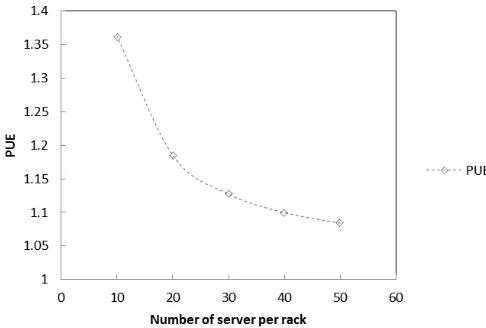
VII. PUE FOR DIFFERENT NUMBER OF SERVERS

In previous section the PUE is determined for a full rack with 50 servers. This section investigates the effect of decreasing the number of servers in a rack on the PUE. The pressure drop per server is 638 Pa. However, the flow rate passing through the rack is varying based on the number of servers. This affects the power that is required by the pumps as shown in equation.

Where, Pps is the pumping power ∆Ps is the pressure drop

across the rack, Qins is the flow rate between the rack and

buffer heat exchanger, is the pump efficiency. In this section, the number of servers per rack is changing from 10 to 50 servers and based on that the rack cooling load start from 1,000 to 5,000 W. The required pumping power to circulate the water between the rack and buffer heat exchanger is varying from 0.8 to 20 W. The power of circulating the water between the buffer heat exchanger and the dry air cooler heat exchanger, Ppr, is again assumed to be double, Pps. The fan

power of the dry air cooler is unchanged.

the full rack load of 50 compared to a 20% partial rack load. Increasing the number of servers per rack decreases the PUE since the power required for the pumps, is not significantly changing with number of servers added.

Fig 9. Variation of PUE by changing the number of the servers per rack

VIII.CONCLUSION

The data center cooling system in this study consists of the dry air cooler and buffer heat exchanger to dissipate the heat from a liquid cooled rack. Temperatures in the full heat rejection system are determined by combining empirical data with full CFD simulations and are based on an real geographical ambient temperature used for the dry air cooler, T5, of 19

o

C. The data center cooling system parameters are calculated using MATLAB to obtain the inlet temperature, T1,

and flow rate, Qins, which are used as boundary conditions for

the liquid immersed server model using COMSOL to determine the pressure.

The power of the pumps is determined from the flow rate and pressures drop, which enables the PUE of data center to be calculated, yielding a data center PUE of 1.08. The effect of the PUE for different rack loads is investigated and it is found that the PUE increases by 26% for a rack-server occupancy that is 20% of maximum capacity. This is due the pump power dropping with decreasing pressure drop.

ACKNOWLEDGMENT

This work was inspired by the technological developments of Iceotope Research and Development based in Sheffield [5]. The authors are grateful to Peter Hopton, CEO Iceotope and Yong Qiang Chi, PhD student at University of Leeds for helpful insights.

REFERENCES

[1] Shah, A., et al. Impact of rack-level compaction on the data center cooling ensemble. in Thermal and Thermomechanical Phenomena in Electronic Systems, 2008. ITHERM 2008. 11th Intersociety Conference on. 2008: IEEE.

[2] Greenberg, S., et al., Best practices for data centers: Lessons learned from benchmarking 22 data centers. Proceedings of the ACEEE Summer

Study on Energy Efficiency in Buildings in Asilomar, CA. ACEEE, August, 2006. 3: p. 76-87.

[3] American Society of Heating, R. and A.C. Engineers, Liquid Cooling Guidelines for Datacom Equipment Centers: ASHRAE Data com. 2006: American Society of Heating, Refrigerating and Air-Conditioning Engineers.

[4] Hopton, P. and J. Summers. Enclosed liquid natural convection as a means of transferring heat from microelectronics to cold plates. in Semiconductor Thermal Measurement and Management Symposium (SEMI-THERM), 2013 29th Annual IEEE. 2013: IEEE.

[5] Chester, D., et al., Cooled electronic system. 2013, Google Patents. [6] Jensen, I.S. Weather statistics for Leeds, England (United Kingdom).

2013 [cited 2014 19/03]; Available from: http://www.yr.no/place/United_Kingdom/England/Leeds/statistics.html. [7] Iyengar, M., et al. Server liquid cooling with chiller-less data center

design to enable significant energy savings. in Semiconductor Thermal Measurement and Management Symposium (SEMI-THERM), 2012 28th Annual IEEE. 2012: IEEE.

[8] 42U. Hot-Aisle/Cold Aisle Layout for Data Center Racks. 2014; Available from: http://www.42u.com/cooling/hot-aisle-cold-aisle.htm. [9] Nada, S., Natural convection heat transfer in horizontal and vertical

closed narrow enclosures with heated rectangular finned base plate. International journal of heat and mass transfer, 2007. 50(3): p. 667-679. [10] Çengel, Y.A., R.H. Turner, and J.M. Cimbala, Fundamentals of

thermal-fluid sciences 2008. p. 534.

[11] Phan-Thien, Y.L., Nhan, An optimum spacing problem for three chips mounted on a vertical substrate in an enclosure. Numerical Heat Transfer: Part A: Applications, 2000. 37(6): p. 613-630.

[12] Chi, Y.Q., Jonathan Summers, Peter Hopton, Keith Deakin, Alan Real, Nik Kapur and Harvey Thompson, Case Study of a Data Centre Using Enclosed, Immersed, Direct Liquid-Cooled Server, in Semiconductor Thermal Measurement and Management Symposium (SEMI-THERM). 2014, IEEE.

[13] Holman, J., Heat transfer, 9th. 2002, McGraw-Hill. p. 335-337. [14] Zitzmann, T., et al. Simulation of steady-state natural convection using

CFD. in Proc. of the 9th International IBPSA Conference Building Simulation 2005. 2005: Montréal: IBPSA.

[15] Rundle, C. and M. Lightstone. Validation of turbulent natural convection in a square cavity for application of CFD modelling to heat transfer and fluid flow in atria geometries. in 2nd Canadian Solar Buildings Conference, Calgary. 2007.

[16] Aounallah, M., et al., Numerical investigation of turbulent natural convection in an inclined square cavity with a hot wavy wall. International Journal of Heat and Mass Transfer, 2007. 50(9): p. 1683-1693.

[17] Wilcox, D.C., Turbulence modeling for CFD. Vol. 2. 1998: DCW industries La Canada, CA.

[18] Rouse, M. power usage effectiveness (PUE). April 2009 [cited 2014 23

March]; Available from:

http://searchdatacenter.techtarget.com/definition/power-usage-effectiveness-PUE.

[19] Haywood, A., et al., Thermodynamic feasibility of harvesting data center waste heat to drive an absorption chiller. Energy Conversion and Management, 2012. 58: p. 26-34.

[20] BELADY, C. The green grid data centre power efficiency metrics: PUE and DCiE. White paper # 6. 2007; Available from: http://www.thegreengrid.org/~/media/WhitePapers/White_Paper_6_-_PUE_and_DCiE_Eff_Metrics_30_December_2008.pdf?lang=en. [21] Incropera, F.P., A.S. Lavine, and D.P. DeWitt, Fundamentals of heat

and mass transfer. 2011: John Wiley & Sons.

[22] Stone, T.L. ENERGY EFFICIENCY IN PUMPING TECHNOLOGY. 2012 [cited 2014; Available from:

http://www.dovercorporation.com/globalnavigation/our-markets/fluids/energy-efficiency-in-pumping-technology.

[23] Serth, R.W., Process heat transfer: principles and applications. 2007: Elsevier Academic Press New York.