Relative Performance Evaluation of Single Chip CFA Color Reconstruction Algorithms Used in Embedded Vision Devices

Relative Performance Evaluation of Single Chip CFA

Color Reconstruction Algorithms Used in Embedded

Vision Devices

B. Mahesh

Asst. Prof, Sagar Institute of Technology, Chevella.India

K. Venkatesh

PG Student,

Prakasham Engineering College

S. Ravi Kumar

PG Student, REC, Warangal

K. Koteswara Rao

Asso.Prof,

PEC

B. Prabhakar Rao

Professor and HOD, Deptt. of ECE,

Sagar Institute of Technology, Chevella, RR, Hyd, AP, India

C. Raja Rao

Dy. Director of Cstern Region, (Under MHRD, Dept. of Higher Education, Govt. of India), Kolkata

Abstract–Most digital cameras use a color filter array to capture the colors of the scene. Sub-sampled (Down sampled) versions of the red, green, and blue components are acquired using Single Sensor Embedded vision devices with the help of Color Filter Array (CFA)[1]. Hence Interpolation of the missing color samples is necessary to reconstruct a full color image. This method of interpolation is called as Demosaicing (Demosaicking). Least-Square Luma–Chroma demulti-plexing algorithm for Bayer demosaicking [2] is the most effective and efficient demosaicking technique available in the literature. As almost all companies of commercial cameras make use of this cost effective way for interpolating the missing colors and reconstructing the original image, the demosaicking arena has become a vital domain of research of embedded color vision devices[3]_{.Hence, in this paper ,the}

authors aim is to analyze ,implement and evaluate the relative performance of the best known algorithms. Objective empirical value prove that LSLCDA is superior in performance.

Keywords – Luminance (Green) Channel, Chrominance (Redandblue) Demosaicking, Bayer Pattern, Least Square, MSE, PSNR.

I. I

NTRODUCTION

Digital color Imaging and processing has become vital because-color image contains more information than grey scale image, and significant use of digital images over internet, and publishing and visualization. Digital color imaging is used in extracting features of interest in an image, and it simplifies object identification. Moreover, if the image analysis is manual, the significant factor is that the humans can discern thousands of color shades and intensities, compared to about only two dozen shades of gray. Thus Digital imaging devices have gained importance over traditional film cameras. Images are formed in a camera in a manner similar to image formation in the eye. However accommodation to image closer objects is done differently in the eye and camera. Human Visual System is the best model and basis for all Vision systems [2].

Embedded color vision devices are different from film cameras. These are preferred to film cameras because they are better, faster, and cheaper.

II. R

EVIEW OF

D

EMOSAICKING

A

LGORITHMS

The performance of a demosaicking algorithm is of utmost importance to how good a digital camera can perform. A lot of existing demosaicking algorithms have been developed. What problems do these demosaicking algorithms try solve? How different are these algorithms in terms of implementation and performance? These are some of the first questions any engineer who wishes to design a novel-demosaicking algorithm, or choose an algorithm to use, have to try to answer. Besides, computational cost does also matter. In attempt to answer part of these questions and thus to arrive at a conclusion in choosing an efficient, easy to implement and cost effective demosaicking algorithm, five different demosaicking algorithms: 1.Bilinear Interpolation 2. Edge Sensing Interpolation-I, Edge Sensing Interpolation-II 3.Color Interpolation Using Alternating Projection 4.High Quality Linear Interpolation Algorithm are considered. 5.Least Square Algorithm. These five demosaicking algorithms are studied qualitatively and implemented for quantitative results. MATLAB is used for implementation.

“Demosaicking” is the process of translating the Bayer

array of primary colors into a final full-color image. The minimum number of cells is 2X2, but this reduces resolution. To correct this variety of image processing algorithms perform colour reconstruction by estimating color using neighboring pixels[5].

A. Bilinear Interpolation

R11 G12 R13 G14 R15 G21 B22 G23 B24 G25 R31 G32 R33 G34 R35 G41 B42 G43 B44 G45 R51 G52 R53 G54 R55

Fig.1. Sample Bayer CFA

From Fig.1, At a Blue (B) center, we need to estimate the Green (G) and Red(R) components. Consider pixel B44at which only B is measured; we need to determine G44. One estimate for G44is given by

4

G54) G45 G43 (G34

G44    

(1)

To determine R44, given R33,R35,R53,R55the estimation for R44is

4

R55) R53 R35 (R33

R44   

Copyright © 2013 IJECCE, All right reserved And at a Red center, we would estimate the Blue and

Green accordingly. Estimating Blue and Green samples at R33Repeating the process at each photo-site (location on the CCD), we can obtain three color. Determining B33 given B22, B24B42and B44given by

4

B44) B42 B24 (B22

B33    (3)

Similarly estimating G33, given G23,G32,G34and G43 given by 4 G43) G34 G32 (G23

G33    (4)

Planes for the scene, which would give us one possible demosaicked form of the scene. This type of interpolation is a low pass filter process. The band-limiting nature of this interpolator smoothen edges, which show up in color images as fringes (referred to as the zipper effect)[6].

B. Edge Sensing Interpolation:

1. Edge Sensing Interpolation Algorithm I

It is observed that in the earlier algorithms most of the color interpolation is done by averaging neighboring pixels indiscriminately. This causes an artifact -- the "zipper effect" in the interpolated image. To combat with this artifact, it is natural to derive an algorithm that can detect local spatial features present in the pixel neighborhood and then makes effective choices as to which predictor to use that neighborhood. The result is a reduction or elimination of "zipper-type" artifacts. And algorithms that involve this kind of "intelligent" detection and decision process are referred as adaptive color interpolation algorithms [7].With reference to Interpolation of green pixels: First, define two gradients, one in horizontal direction, and the other in vertical direction, for each blue/red position. For instance, consider B8: define two gradients as

G24

G22

ΔH





(5)

G33

G13

ΔV





(6)

Where | . | denotes absolute value. Define some threshold value T. The algorithm then can be described as follows:

If



H

< T and



V

>T (7)

      2 G24 G22 G23 (8) Else if



H

>T and V< T (9)

      2 G33 G13 G23 (10) Else         4 G33 G24 G22 G13 G23 (11) End

The choice of T depends on the images and can have different optimum values from different neighborhoods. A

particular choice of T is

2

ΔV ΔH

T 

(12) In this case, the algorithm becomes:

If



H

<



V

,

      2 G24 G22 G23 (13)

Else if



H

>



V

_,

      2 33 13

23 G G

G (14) Else         4 G33 G24 G22 G13 G23 (15 ) End

2. Edge Sensing Interpolation Algorithm II:

A slightly different edge sensing interpolation algorithm is described as. Interpolation of green pixels: Same as in edge sensing interpolation algorithm-I except that horizontal and vertical gradients are defined differently. From fig.1 to estimate G44 at B44, we define gradients as:

2 B46 B42 B44

ΔH  

(16)

2 B64 B24 B44

ΔV  

(17) The actual algorithm follows as in the edge sensing interpolation algorithm I. Interpolation of red/blue pixels: Similar to bilinear interpolation algorithm, except that, colour difference is interpolated instead of color itself.

C.

Colour

Interpolation

Using

Alternating

Projections:

In digital cameras that use the Bayer Pattern filter array, the green channel is sampled at higher frequencies than the red and blue channels. Therefore, details in the green channel are better preserved than in the red and blue channels since the green channel is less likely to be aliased. Interpolation of the red and blue channels thus becomes the limiting factor in performance. In particular, colour artifacts caused by aliasing in the red and blue channels are very severe at high frequency regions such as edges. The objective of this algorithm is to reduce the amount of red and blue channel aliasing by using an alternating-projection scheme that uses inter-channel correlation effectively. The block diagram of the algorithm is shown below, and details of the algorithm are explained [8].

D. High Quality Linear Interpolation Algorithm:

Classical bilinear interpolation methods use only the color information in the channel to be interpolated. For example, when a green pixel is to be estimated, classical methods usually use only information in the green channel. In this high-quality linear interpolation method it combines bilinear interpolation with a gradient-correction gain and turns out a better estimation of the missing color information [9]. Specifically, to interpolate G values at an R location, use the formula:

j)

(i,

αΔ

j)

(i,

g

ˆ

j)

(i,

g

ˆ



_B



_R (18)

Where

g

ˆ

_B is the bilinear interpolation and



_Ris the gradient of R computed by



       (2,0)} 2,0), ( (0,2), 2), {(0, n) (m,

R r(i m,j n)

4 1 j) r(i, j) (i, Δ (19)

For interpolating G at blue pixels, the same formula is

j)

(i,

βΔ

j)

(i,

r

ˆ

j)

(i,

r

ˆ



_B



_G (20)

With



_G

( j

i

,

)

determined by a 9-point region. For

interpolating R at blue pixels, use the formula

j)

(i,

γΔ

j)

(i,

r

ˆ

j)

(i,

r

ˆ



_B



_B (21)

With



_B

( j

i

,

)

computed on a 5-point region. The formulas for interpolating B are similar, by symmetry. To determine appropriate values for the gain parameters

{α,β,γ}, we used a Wienerapproach; that is, we computed the values that lead to minimum mean-square error interpolation, given second order statistics computed from a good data set. We then approximated the optimal Wiener coefficients by integer multiples of small powers of 1/2, with the final result α = 1/2, β = 5/8, and γ = 3/4. From the values of {α,β,γ} we can compute the equivalent linear

FIR filter coefficients for each interpolation case. The resulting coefficient values make the filters quite close (within 5% in terms of mean-square error) to the optimal Wiener filters for a 5×5 region of support. This sub-sampling approach is not really representative of digital cameras, which usually employ careful lens design to effectively perform a small amount of low-pass filtering to reduce the aliasing due to the Bayer pattern sub-sampling. However, since all papers in the references perform just sub-sampling, with no low-pass filtering, we did the same so we could compare results. We has also tested all interpolation methods with small amounts of Gaussian low-pass filtering before Bayer sub-sampling, and found that the relative performances of the methods are roughly the same, with or without filtering. The improvement in peak-signal-to-noise ratio (PSNR) over bilinear interpolation.

E. Least-Squares Luma

–

Chroma Demultiplexing

Algorithm for Bayer Demosaicking:

The algorithm for Bayer demosaicking by adaptive luma–chroma demultiplexing used in this paper is precisely the one described in ; it is summarized here for completeness. We assume that an underlying color image with RGB components fR,fG and fB is sampled on the

rectangular integer lattice Λ=Z2 with the upper left point of the image at coordinate (0,0). The unit of length used in this paper is the vertical spacing between sample elements in the CFA signal, denoted 1 px. The standard spatial multiplexing model of the BayerCFAsignal. n _,n =

f n ,n m n ,n + f n ,n m n ,n +

f n ,n m n,n (22)

=

[ 1, 2](1 − (−1) (1 + (−1) ) +

[ 1, 2](1 + (−1) + [ 1, 2](1 +

(−1) (1 − (−1) (23)

This expression offers a different interpretation to the spatial representation of the Bayer CFA signal. Specifically, the CFA is treated as the multiplexing of one baseband signal and two modulated difference signals. The baseband signal fL identifies an achromatic luma component and the two modulated signals fC1 and fC2 identify two separate chromatic color difference

components, referred to here as chroma components. Substituting for -1=e

j



in equation , one obtains

n ,n = f n ,n + f n,n e ( ) +

f n ,n (e − e ) ≜ f n ,n + f n ,n

+f n ,n + f n ,n (24)

With Fourier transform

fCFA(u, v) = FL(u, v) + Fc1(u − 0.5, v − 0.5) +

Fc2(u, v − 0.5) (25)

Where, frequencies are expressed in c/px.

Least-Squares Filter Design:

We have seen that the estimate for component X ∈

{C1m, C2ma, C2mb} is obtained by the spatial filtering

operation[10] fX = fCFA*hX’ where x ∈

{1,2a, 2b}respectively. Suppose we have a model for the

original signal fXso that the difference between fXand fX can be expressed as a stationary random field. Then, a suitable design criterion is to minimize the expected

squared error, resulting in the

filter h = arg min E(f [n , n ] − (f ∗ h)[n , n ]) ] which is independent of (n1; n2) due to stationarity. Because good models for fX do not exist yet,we can instead compile a set of training images from typical color images and compute filters that minimize squared errors over the training set; these filters are the solution to standard least-squares problems[11] . Assume that we have chosen a training set of original RGB color images. Thus, we also have access to the signals fC1m, fC2ma and

fC2mb, which are respectively the original baseband signals

fC1 and fC2 modulated to the appropriate centering

frequencies. Let us first consider C1 and filter h1. Recall that the estimate f(i)C1mfor the i

th

training image is obtained by f(i)C1m= f(i)CFA*h1. If h1 has region of support B that is

a subset of the ithimage sampling raster Λi, then

( ) = ∑[ , ]∊ ℎ1[ 1, 2] ( )[ 1 − 1, 2 − 2 ]

⋀ ₍₂₆₎

Fig.2. Block diagram of adaptive luma-chroma demultiplexing algorithm for the Bayer CFA structure.

We define the total squared error (TSE) on C1 over every pixel in a training set of K images by

1 = ∑ (f( )_{c [n1, n2] − f}( )_{c [n1, n2](27)} [ , ]∈∆

The least-squares filter h1*that minimizes the estimation error on C1 is the solution to the least-squares problemℎ1∗= arg min TSE c1

We can reformulate the least-squares problem using matrices. Let NB = |β| be the number of h1 filter coefficients and let NW=|Λi| be the number of pixels in the

Copyright © 2013 IJECCE, All right reserved every training image. We may reshape f(i)C1minto a NW×1

column vector f(i)C1mby scanning f (i)

C1mcolumn-by-column

over Λi. Now, reshape h1into a NB×1 column vector h1by scanning h1column-by-column over B. Finally, construct a NW×NBmatrix A(i)by scanning f(i)CFAin alignment with h1 such that each entry of the matrix product A(i)h1 realizes

equation . The result of A(i)h1is the NW×1 column vector f (i)

C1m aligned pixel-wise with f (i)C1m. These matrices

reformulate equation into

1

( )

* ( ) 2

1 | 1

1

a r g m i n | | | |

i k

i

i C m C m

h i

h f f











(28)

1

( ) ( ) 2 1 1 | 1

a r g m i n | | | |

k

i i

h C m

h i

A f









(29) Which is a standard least-squares problem with solution

1

* ( ) ( ) ( ) ( )

1 1

1 1

T T

k k

i i i i

c m

i i

h A A A f



 

   

 _  _ _  _

(30)

Finally, we reshape

h

*_i back onto support B to get the

least squares filter

h

*_i.The same framework is used on C2

to obtain the least squares filters h2aand h2bdefined over supports D’ and D0 (where D0 is the transpose of D’). Here, we have

    2

( )

( )

2 2 2

1 [ 1 , 2

1, 2 1, 2

i

i k

i

c C m C m

i n n A

T S E f n n f n n



 

 

   

 

 

(31) The set of weighting coefficients wi is obtained in the same manner described previously. The sets wiand (1−wi) are modulated accordingly to match the centering frequencies of fC2maand fC2mb respectively. As before, we cast the least-squares problem into matrix form. Furthermore, we can simultaneously find the least squares

filters

h

*_{2 a} and

h

*_2b by temporarily merging the two

filter kernels. Once again, let NW =|Λi| be the number of pixels in the ithtraining image and assume NW to be the

same for all images. Let ND= |D| be the number of h2a(or h2b) filter coefficients. First, reshape f

(i)

C2m into a NW×1

column vector f(i) C2m by scanning f(i)C2m

column-by-column over Λi. Next, reshape h2aand h2binto two ND×1

column vectors h2a and h2b respectively by scanning

column-by-column and then stack h2aover h2bto form the 2ND×1 column vector

ℎ = [ℎℎ ] (32)

Finally, construct a NW×2NDmatrix B(i)by scanning the

product values of f(i)CFA and modulated weighting

coefficients in alignment with h2 such that each entry of the matrix product B(i)h2 realizes equation . The matrix

product is the NW×1 column vector

( )

2 i

C m

f



aligned

pixel-wise with f(i)C2m. With these matrices we can express the

standard least-squares problem on C2 as

( )

2 2

2 2

* ( ) 2

2 2

1 ( )

( ) 2 2

1

a r g m i n | | | |

a r g m i n | | | |

i

C m

C m

k

i C m h

i k i

i h h

i

h f f

B f







 

 





(33) 1

* ( ) ( ) ( ) ( )

2 2

1 1

T T

k k

i i i i

C m

i i

h B B B f



 

   

 _



_ _



_

(34)

Now extract h*2a from the first ND entries of h*2 and

h*2bfrom remaining entries and then reshape h*2aand h*2b

separately back onto supports D and D1to get the least-squares filters h*2a and h*2b. We have relied on the

assumption that each training image has the same number of pixels. Although this may not be true in general, we can enforce this assumption by dividing each training image into images of the same dimensions. Then, the sub-image size NW is constant for each piece and we train over all sub-images instead. In the sub-image window has dimensions 96 pixels×96 pixels giving NW = 9216

pixels[12]. The choice of NW has negligible effect on the

demosaicking results.

III. R

ESULTS AND

D

ISCUSSIONS

In this section, we are applying five different algorithms to five different images as shown in fig.3.The results can be calculated using MATLAB simulation with both subjective & objective measures MSE & PSNR. The following figure & tables will give the results. Table 1 represents the MSE values of all five images & Table 2 represents the PSNR values of all five images. The fig4,5 represents the corresponding MSE&PSNR and averages of image1.similarily,for images2,3,4,5 corresponding figures can be represented as same as below.

Fig.3 1, 2, 3, 4, 5: Original Data Set. Fig.3a A, B, C, D, E: Bilinear Interpolation

Fig.3b F, G, H, I, J: Edge Sensing Algorithm.

Fig.3c K, L, M, N,O: High Quality Linear Interpolation Algorithm.

R

ESULT

T

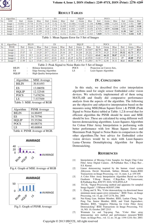
ABLES

Table 1: Mean Square Error for 5 Set of Images

Table 2: Peak Signal to Noise Ratio for 5 Set of Image

BILIN : Bilinear Interpolation POCS : Projection on Convex Sets,

ES : Edge Sensing Algorithm LS : Least Square Algorithm

HQLIP : High Quality Interpolation

Algorithm MSE Average

BILIN 30.81493

ES 13.08058

HQLIP 12.32548

POCS 7.678256

LS 7.537509

Table 3: MSE Average of RGB

Algorithm PSNR Average

BILIN 16.88495

ES 34.75796

HQLIP 35.55286

POCS 40.08376

LS 40.66864

Table 4: PSNR Average of RGB.

Fig.4. Graph of MSE Average of RGB

Fig.5. Graph of PSNR Average

IV. C

ONCLUSION

In this study, we described five color interpolation algorithms used for single sensor Embedded color vision devices. We selectively implemented all of them using MATLAB and finally did comparative performance analysis from the aspects of the algorithm. The following are the objective and subjective interpretation based on the measures using MSE(Mean Square Error ) & PSNR (Peak Signal to Noise Ratio) tabled at Table: 1,2.It reveal that for efficient algorithm the PSNR should be more and MSE should be less .These are calculated by using different well known demosaicking algorithms. Least-Squares Algorithm for Colour Filter Array Interpolation is performing with better performance with low Mean Square Error and Maximum Peak Signal to Noise Ratio in comparison to the other algorithms.The best advice for Embedded color vision devices would be to stick with Least-Squares Luma–Chroma Demultiplexing Algorithm for Bayer Demosaicking.

R

EFERENCES

[1] Interpolation of Missing Color Samples for Single Chip Color Filter Array Digital Camera , B.Prabhakar Rao, C.Raja Rao , S.S. Kumar.

[2] Linear demosaicing inspired by the human visual system Alleysson, David; Süsstrunk, Sabine; Hérault, Jeanny,IEEE Transactions on Image Processing, vol. 14, num. 4, p. 439-449. [3] A Color Filter Array Interpolation Algorithm Based on Color

Gradients V.Roop Kumar, C.Raja.Rao, K.Veeraswami, B.Prabhakar Rao, RTCTV 2010, VCE,HYD,A.P.

[4] D.Cok, “Signal Processsingmethod and apparatus for sampled Image Signals”, USPatent 4630307,1986

[5] L. Zhang and X. Wu, “Color demosaicking via directional linear minimum mean square-error estimation,” IEEE Trans. on Image Processing, vol. 14, pp. 2167-2178, Dec. 2005.

[6] Nai-Xiang Lian, Student Member, IEEE, Lanlan Chang, Yap-Peng Tan, Senior Member, IEEE, and Vitali Zagorodnov, Member, IEEE, “Adaptive Filtering for Color Filter Array Demosaicking” IEEE Transactions on Image Processing, Vol. 16, NO. 10, October 2007 2515.

[7] Wenmain Lu and Yap-peng Tan, “Color filter array demosaicing: new method and performance measures”IEEE Trans. on Image Proc., vol. 12, no. 10, pp. 1194-1210, Oct. 2003.

0 20 40

AVARAGE

AVARAGE

0 50

AVARAGE

Copyright © 2013 IJECCE, All right reserved [8] D. Menon, S. Andriani, and G. Calvagno, , "Demosaicing with

Directional Filtering and a Posteriori Decision", IEEE Trans. on Image Processing, vol. 16 no. 1, Jan. 2007.

[9] B. K. Gunturk, Y. Altunbasak and R. M. Mersereau, ``Color plane interpolation using alternating projections ,'' {\em IEEE Trans. on Image Proc.}, vol. 11, no. 9, pp. 997-1013, Sep. 2002. [10] X. Li, "Demosaicing by successive approximation", IEEE

Transactions on Image Processing, VOL. 14, NO. 3, MARCH 2005

[11] H. S. Malvar, L.-W. He, and R. Cutler, “High-quality linear interpolation for demosaicing of Bayer-patterned color images”, IEEE International Conference on Acoustics, Speech, and Signal Processing, Montreal, Canada, May 2004.

[12] Glaude A. Laroche and Mark A. Prescott, “Apparatus and method for adaptively interpolating a full color image utilize chrominance gradients,” U.S. Patent 5,373,322,Eastman Kodak Company, 1994.

[13] Xiaolin Wu, Senior Member, IEEE, and Ning Zhang “Primary-Consistent Soft-Decision Color Demosaicking for Digital Cameras (Patent Pending)” IEEE Transactions on Image Processing, VOL. 13, NO. 9, Sept,2004, pp1263 to 1274

A

UTHOR

’

S

P

ROFILE

Mahesh. B

received B.Tech.(ECE), M.Tech. (CSE) from JNTU Hyderabad, India. At present he is an Assistant Professor (CSE) at Sagar Group of Institutions, Hyderabad, India. His Research in Image Processing is Demosaicking, and Simplified image compression algorithm for Bayer filter array.

Venkatesh. K

received the B.Tech. (ECE) from Nimra college of Engineering & Technology, Vijayawada. He is currently doing M.Tech in VLSI & EMBEDDED SYSTEMS from Prakasam College of Engineering, kandukur, JNTUK.

Ravi Kumar. S

received B.Tech. (CSE), currently, pursuing M.Tech, from JNT University HYD. His research interests include image and Video processing, pattern recognition, computer vision, and color imaging.

Koteswara Rao. K

received the B.E degree from Andhra University College of Engineering in 2002. He worked as Assistant Professor at Prakasam College of Engineering between 2002 to 2008.He received M.Tech from Jawarharlal Nehru Technology University Hyderabad in 2008-2011. He is currently doing Associate Professor since 2011 at Prakasam College of Engineering, Kandukur.

Prabhakar Rao. B

Obtained B.Tech. (ECE) from Nagarjuna University, M.Tech. (I&CS) from University College of Engineering, JNTUK and M.Tech (Embedded Systems) from JNTUH, at present a Professor and HOD, Dept., of ECE, Sagar Institute of Technology, Chevella, Hyd, A.P, India. So far he rendered his services in various capacities as Asst. Prof, Asso. Prof and Vice Principal in various Engg., Institutions. His areas of interest include Machine Vision, Bionic Eye, VLSI Implementation of IP Algorithms, and Cost Effective Image Reconstruction.

Shri. C. Raja Rao

obtained his B.E in ECE from Andhra University in 1995 and M.Tech in DSCE from JNTU Hyderabad in 2001. At present he is working as Deputy Director

of Training in Board of Practical Training (Eastern