r
Water Mass Changes
in
the North and
South Pacific oceans between the 1960s
and 1985-94
Annie Pik Shan WONG
BSc (Hons.)
University of New South Wales
MPOSc
University of Tasmania
A thesis submitted in fulfilment of the requirements for the degree of Doctor of Philosophy, Institute of Antarctic and Southern Ocean Studies,
University of Tasmania, Australia.
Statement
This thesis contains no material which has been accepted for the award of any other degree or diploma in any tertiary institution, and that, to the best of my knowledge and belief, this thesis contains no material previously published or written by another person, except where due reference is made in the text of the thesis.
Abstract
Comparisons have been made along five modern hydrographic sections against historical hydro graphic data to investigate water mass changes in the North and South Pacific oceans. The five modern hydrographic sections were sampled in the decade 1985-94, while the historical data were mostly from the late 1960s. Below the seasonal mixed layer, statistically significant temporal differences in temperature and salinity have been detected in the water masses that occur in the top 2000 dbar of the water column. These differences in water mass properties are assumed to result from sea surface changes at the formation regions.
Of all the water mass changes, the most spatially coherent ones come from the shallow salinity maxima of North Pacific Subtropical Water (NPSTW) and South Pacific Subtropical Water (SPSTW), and the intermediate salinity minima of North Pacific Intermediate Water (NPIW) and Antarctic Intermediate Water (AAIW). The two shallow salinity maxima, NPSTW and SPSTW, have shown signs of salinity increase, while the two intermediate salinity minima, NPIW and AAIW, have become fresher and, except along l 7°S, have become warmer. Since NPSTW and SPSTW originate under the high evaporative cells of the subtropical North and South Pacific, and NPIW and AAIW acquire their properties near the polar gyres, these changes in the ocean interior imply an increase in net evaporation over the mid-latitudes, and an increase in net precipitation over the high-latitudes in both hemispheres. Together these results imply a strengthening of the hydrological cycle over the North and South Pacific oceans.
Outputs from a coupled climate model show that under increasing atmospheric C02 , the model ocean responds with a warming of the water column in the top
300 dbar. Superimposed on this background warming trend is a decrease in salin-ity in the two intermediate salinsalin-ity minima of the Pacific (NPIW and AAIW), and corresponds to near-surface freshening where their respective isopycnals outcrop. Hence the freshening signature that has been detected in NPIW and AAIW from observational data is qualitatively consistent with this climate model's response to increasing C02 • However, natural variability cannot be discarded as a possible cause for the observed changes.
Acknowledgements
This project was carried out under a National Greenhouse Advisory Commit-tee PhD scholarship, with extra resources provided by the Antarctic Cooperative Research Centre. I wish to thank these organisations for their support.
The data presented in this thesis have been collected by many scientists, technicians, officers and crew on many research ships over many decades, collated and disseminated by various oceanographic institutions. I am grateful to these people, for our knowledge of the ocean is built on their patient effort in collecting these scientific data.
I wish to thank my two supervisors, Nathan Bindoff and John Church, without whose insightful comments and technical expertise, this project would have a very hard time coming into focus, let alone to fruition. Their revitalizing interest in the topic of ocean climate change has added much spark to this research.
The following people are gratefully acknowledged for providing patient dis-cussions on various technical topics: Dave Jackett on neutral surfacing; Trevor McDougall on things that no one dares ask; Sue Wijffels on various facets of the Pacific; Tony Hirst, Bill Budd and Xingren Wu on the coupled climate model; and James Patterson on almost every computer and printer problem I have had. I would also like to acknowledge Dr .Harry Bryden for providing the WOCE P21 data, and Dr.Tony Hirst for providing the averaged CSIRO model output.
On a personal level, thanks to all the friendly faces around IASOS, and to those who I have hiked and climbed and got drunk with in Tassie over the past eight years. Inspirations have come from strange places.
Contents
1 Introduction
1.1 Detection of decadal changes .
1.2 Observations of changes in the ocean interior .. 1.3 Natural variability in the Pacific climate system 1.4 Objectives and layout of the thesis . . . .
1 1
3 7
g
2 A method for analysing temporal changes in hydrographic data 11 2.1 Water mass properties and subduction . . . 11 2.2 The relations between fJ-S changes on isobars and on isopycnals 13 2.3 Three "pure" processes responsible for the changes 15
2.3.1 Pure warming (cooling) 15
2.3.2 Pure freshening (salinification) . 2.3.3 Pure heaving . . . . 2.4 The role of the stability ratio, Rp . . .
2.5 Decomposing water mass changes into three components
3 Observational data sets and treatment of data 3.1 Observational data sets . . . .
3.1.1 Historical hydrographic data sets 3.1.2 Modern WOCE transects
3.2 Treatment of data . . . .
3.2.1 Vertically interpolating to neutral surfaces
3.2.2 Laterally interpolating to the WOCE coordinates 3.2.3 Calculating Rp and the six variables . . .
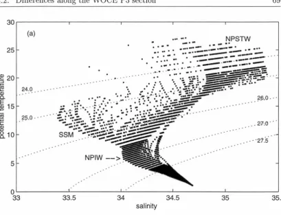
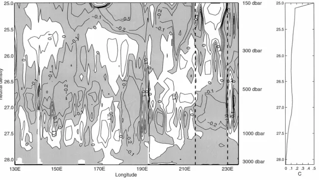
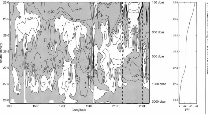
4 Observed changes in the North Pacific Ocean 4.1 Differences along the WOCE Pl section
4.2 Differences along the WOCE P3 section 4.3 Differences along the WOCE P4 section
16
17
17
20
25 25 25 28 30 30 32 34
4.4 Summary and Discussion for the North Pacific Ocean
. . .
110~
5 Observed changes in the South Pacific Ocean 117
5.1 Differences along the WOCE P21 section . . . . 117 5.2 Differences along the WOCE P16 section . . . . 142 5.3 Summary and Discussion for the South Pacific Ocean 169
6 Response of a model ocean to increasing atmospheric C02 173 6.1 Model data
. . .
174 6.2 The model ocean's response to increasing C02 . . . 181 6.3 Comparing the model's response with observations 203 6.4 Summary o 0 0 o 0 0 o o o o o o o o o o o 0 0 0 I 0 0 2077 Discussion 209
7.1 Pacific freshwater content change 209
7.2 Pacific heat content change . 219
7.3 Pacific steric height change . 225
8 Conclusions and Scope for future work 229
1
A Using the three "pure" processes to derive a linear system 232
B Objective mapping procedure 236
Chapter
1
Introduction
1.1
Detection of decadal changes
In recent years, there is a growing focus on documenting loi;g-term, large-scale variability and changes in the earth's climate system, in an attempt to detect climate change "signals" caused by the enhanced greenhouse effect. Most of these studies have focused on surface air temperature as a single study parameter. These studies range from using large-scale averaging methods for investigating long-term mean trends (e.g. Jones (1988)), to using pattern-based methods for comparing spatial patterns of change in observations with those from model forecasts (e,g. Barnett and Schlesinger (1987), Parker et al. (1994)).
Pattern-based methods are part of the so-called "fingerprint" method. The fingerprint method involyes the identification of a multivariate signal that is unique to the enhanced greenhouse effect (e.g. Santer et al. (1995)). The multivariate signal can involve several parameters at one location, or a single parameter at several locations, or several parameters at several locations. For example, Karoly et al. (1994) used the zonal mean atmospheric temperature change (one par'kmeter) as a function of height and latitude (several
lo~ations)
to define their multivariate signal.Similar pattern-based detection of multivariate signals in the ocean interior has not been carried out on a global basis, primarily because of the limited availability of long-term, large-scale oceanographic observations. However, it is important to study decadal-scale changes in the ocean because not only is the ocean an integral part of the climate system, but it also plays an important role in modifying the global distribution of heat and freshwater. In model experiments with increasing greenhouse gas forcings, certain qualitatively consistent changes are apparent in the ocean circulation, e.g. reductions in deep
1.1. Detection of decadal changes
water formation in the North Atlantic (e.g. Mikolajewicz et al. (1990)). However, it is not clear how the properties of the water masses that are responsible for inter-basin exchange of heat and salt will alter under the enhanced greenhouse effect.
2
All waters in the world's oceans have characteristics that ultimately are the results of atmospheric conditions at the sea surface from some point in time, that have subsequently been modified along the subduction paths. The surface conditions that have effects on the water masses of the world's oceans therefore include surface temperature, surface salinity, and surface wind stress curl. Surface temperature and salinity control the strength of the buoyancy-driven convection, as well as give the water masses their potential temperature (
0)
-salinity (S) properties. Surface wind stress curl determines the subduction rates due to Ekman pumping and the wind-driven circulation, both of which are responsible for distributing the water masses (Woods 1985). The circulation of the water masses around the global ocean, and their subsequent mixing, serve to distribute these surface information into the interior of the ocean. Any significant long-term changes to these surface conditions will therefore manifest themselves at some later time in the ocean interior beneath the
seasonally-affected surface mixed layer.
Historically, most large-scale oceanographic studies have attempted to explore the ocean interior with little focus on variability. As data sets have grown in recent years, more emphasis has been placed on studying oceanic variability and long-term changes, with the North Atlantic being the most studied ocean, because of the relatively dense data sets available. Since the mid 1980s, many one-time surveys and repeat surveys have been conducted around the world's oceans under the ,World Ocean Circulation Experiment (WOCE). As a result of WOCE, there are now opportunities to explore long-term interior changes in other ocean basins. This thesis presents the first systematic study of decadal-scale changes in the North and South Pacific oceans, using five one-time hydrographic surveys from WOCE that are situated in areas with dense
1.2. Observations of changes in the ocean interior
1.2
Observations of changes in the ocean
interior
The North Atlantic
3
Most studies that utilize oceanographic observations to document large-scale changes in the ocean's interior have been carried out in the North Atlantic, where several deep-ocean transects have been repeated over the past 20 to 30 years. Based on repeats of two hydrographic lines along 24°30' N and 36°16' N, Roemmich and Wunsch (1984) reported ocean-wide warming in the subtropical North Atlantic, from 700 m to 3000 m, between 1957 /1959 and 1981. Another repeat survey along 24°30' N during 1992 showed that this mid-depth warming had continued, and that the subtropical North Atlantic was responding to wind and buoyancy forcing conditions of the past 35 years
(Parrilla et al. 1994). Bryden et al. (1996) quantified the observed changes along 24°N, and showed that the warming from 1957 to 1981 observed by Roemmich and Wunsch (1984) was principally due to downward displacements of isopycnals, while the continued warming from 1981 to 1992 observed by Parrilla et al. (1994) was more likely the result of changes in the water mass characteristics. A 73-year time-series established using data from a
hydrographic station at Bermuda (western subtropical Atlantic) also shows a long-term temperature increase trend in the 1500-2500 dbar layer (Joyce and Robbins 1996). More recently, Joyce et al. (1999) showed that in the western part of the subtropical gyre between 20°N and 35°N, Labrador Sea Water has become colder and fresher since 1992, and the warming trend observed by Bryden et al. (1996) has continued to 1997.
1.2. Observations of changes in the ocean interior 4
recent changes in the North Atlantic and proposed that winter convection at the three convective renewal sites of the North Atlantic: the Greenland/Iceland Sea, the Labrador Sea, and the Sargasso Sea, evolved in phase but at difference signs during this century, and that this decadal evolution was driven by the North Atlantic Oscillation.
Where repeats of ocean-wide transects are not available, some investigators use historical data where and when the coverage allows for
studying large-scale ocean variability over time. Levitus (1989) composited and compared two pentads of historical hydrographic observations: 1955-1959 and 1970-1974, and found the intermediate depths of the North Atlantic subtropical gyre to be colder and fresher during 1970-1974, compared to 1955-1959. This is different from the result of Roemmich and Wunsch (1984), which spanned another decade after the 1970s. In the subarctic region, Levitus (1989) found that the western half of the North Atlantic have warmed and become more saline, while the eastern half south of Iceland was found to have cooled and freshened. Changes in the subtropical gyre were seen to be consistent with an upward displacement of density surfaces, in contrast to the eastern subarctic gyre, where T-S changes were nearly density-compensating. Thus different phenomena seemed to be responsible for T-S changes in different regions of the North Atlantic.
Antonov (1993) used historical hydrographic station data to construct a set of annual-mean ocean temperature time series for the period 1957-1981, for both the North Atlantic and the North Pacific. While there were large areas in both oceans where cooling trends or warming trends dominated, as a whole, the ocean temperature averaged over the North Atlantic Ocean, from the equator to 70°N, showed warming from 600-700 m to 2500-3000 m, comparable to the result of Roemmich and Wunsch (1984).
The Pacific
1.2. Observations of changes in the ocean interior 5 Ocean is therefore an ideal ocean to test the hypothesis that if any significant changes have occurred in the atmosphere over the Pacific region during the past few decades, then these changes should manifest themselves in the permanent thermocline and the intermediate depths of the Pacific Ocean, while the water mass properties of the deep Pacific should remain largely unchanged. Any deep Pacific changes would therefore imply Southern Ocean changes. Antonov (1993) has observed no significant ocean temperature changes in the North Pacific, averaged from the equator to 60°N, below 500-700 m over the 25 years between 1957-1981. During the same period the North Atlantic has been observed to have warmed from 600-700 m to 2500-3000 m. It was concluded that this asymmetry was due to the different deep water ventilation mechanisms at the two oceans.
The Pacific does not enjoy as many repeat surveys as the North Atlantic. To date, the few repeat hydrographic transects that could be used to study water mass decadal changes are mostly restricted to the western basins. In the North Pacific, the Japanese Meteorological Agency has been repeating an oceanographic survey along the 137°E meridian since 1967 (designated WOCE PR2). Suga et al. (1989) and Suga and Hanawa (1995a) have successfully used this time-series data set to demonstrate that the interannual variability of the volume of North Pacific Subtropical Mode Water is strongly related to the Kuroshio meanders. Using the same data set, Qiu and Joyce (1992) have shown that the subduction of North Pacific Intermediate Water (NPIW) is also
dependent on the Kuroshio meanders. Shuto (1996) found correlations between the interannual variations of the areas of the tropical saline water and NPIW, and the wind-stress curl minimum in the area southeast of Japan.
1.2. Observations of changes in the ocean interior
temperature and salinity changes in the top 300 dbar that could be related to the 1987 El Niiio.
Analysis on isopycnals
6
Ocean processes observed on isobaric surfaces contain effects of heave and Rossby waves. Hence for the purpose of studying water mass property changes, isopycnal surfaces are a more appropriate coordinate system for analysis. In a study concerning the ocean's response to a warmed atmosphere, Church et al. (1991) pointed out the counter-intuitive feature that, in a "warming without salinity change" scenario, the effect of warmed water subducted into the thermocline would be to cause an observed cooling (and corresponding
freshening) on isopycnals. Bindoff and McDougall (1994) expanded this concept and formalised three "pure" processes that could result in subsurface changes in () and S. These three idealised subduction processes are called "pure warming (or cooling)", "pure freshening (or salinification)", and "pure heaving". An inverse approach was employed to distribute any observed subsurface temporal changes into three components, due to these three processes.
By this method, the observations of Bindoff and Church (1992) from the Tasman Sea were interpreted as the result of surface warming in the formation region of Subantarctic Mode Water (SAMW), and surface freshening in the formation region of Antarctic Intermediate Water (AAIW). Johnson and Orsi
(1997) presented more observations on isopycnals from repeats of a meridional line along 170°W (between 1968/9 and 1990), and a zonal line along roughly 35°S (between 1969 and 1991). They supported previous findings by Bindoff and Church (1992) and Johnson et al. (1994): that the observed changes in SAMW and AAIW in the southwest Pacific were consonant with surface
warming and freshening in the southern high latitudes, and that there had been a reduction in strength of the modified NADW between 1987 and 1992.
1.3. Natural variability in the Pacific climate system
1.3 Natural variability in the Pacific climate
system
The Pacific coupled ocean-atmosphere system has been known to exhibit I
decadal variability. Perhaps the most well-known climate phenomenon in the 7
Pacific region is the El Niiio - Southern Oscillation in the equatorial Pacific, which has decadal effects over the rest of the Pacific region and the Southern Ocean. For example, Jacobs et al. (1994) derived from satellite data that
mid-latitude Rossby waves, generated by reflection of an equatorial Kelvin wave from the American coasts in response to the 1982-83 El Niiio, propagated to the northwest corner of the Pacific Ocean a decade later. These Ross by waves appeared to have caused a northward re-routing of the Kuroshio Current, which led to significant increases in SST in the northwestern Pacific during 1991. More recently, White and Peterson (1996) suggested that, through atmospheric teleconnection, El Niiio activities in the equatorial Pacific might have initiated what is now known as the Antarctic Circumpolar Wave observed in the
Southern Ocean'.
One of the better-known examples of coupled ocean-atmosphere variability in the Pacific is the simultaneous changes in SSTs, surface winds and organised convection observed over the tropical Pacific during the 1970s and the 1980s. These anomalies represent a shift in the background state of the coupled ocean-atmosphere system over the tropical Pacific, and seem to have forced changes in the mid-latitude atmospheric circulation (Graham 1994). Tuenberth and Hurrell (1994) provided further evidence that between 1976 and 1988, the North Pacific went through an anomalous period that was characterised by a deep Aleutian low.
To determine the physical mechanisms behind this kind of decadal-scale climate variability, many investigators have analysed data from coupled ocean-atmosphere models. These studies have provided much insight into the ocean's response to external forcings in the Pacific region. Latif and Barnett
1.3. Natural variability in the Pacific climate system 8
gyre to weaken, but because the ocean's response lags behind the wind stress curl change, an oscillatory mode is set up that has a period of decades. By using all historical temperature profiles available at the National Oceanographic Data Center, Zhang and Levitus (1997) observed a clockwise rotation of
temperature anomalies, at 250 m depth, propagating around the entire North Pacific between 1961 and 1990, that resembles the decadal-scale oscillation suggested by Latif and Barnett (1994) and Latif and Barnett (1996).
Evidence from sea surface temperature records shows that the changes that took place in the 1970s and the 1980s in the Pacific are part of a pattern of interdecadal climate variability known as the Pacific Decadal Oscillation (PDO)
(Mantua et al. 1997). The PDO is centred over the mid-latitude North Pacific, and has, during this century alo~e, changed polarity around 1925, 1947 and 1977.
Relatively few studies on similar coupled ocean-atmosphere variability in the South Pacific have been done, partly owing to a lack of data in the region. However, by using NCEP-NCAR reanalysis data, Garreaud and Battisti (1999) have demonstrated that the South Pacific also displays interdecadal
1.4. Objectives and layout of the thesis 9
1.4 Objectives and layout of the thesis
The aim of this thesis is to undertake the first systematic study of decadal changes in the interior of the North and South Pacific oceans, using five newly available trans-oceanic hydrographic surveys from the World Ocean Circulation Experiment (WOCE), and subsequently infer variations in the surface
conditions from the observed subsurface differences. The observed changes are compared with outputs from a coupled climate model with increasing C02 to identify qualitative consistencies between model outputs and observations. Whether climate change can be detected in ocean observations or not,
comparison studies that employ modern large-scale ocean observations, such as the one presented in this thesis, introduce new knowledge about ocean
variability and change. This knowledge is important for validating numerical models that are used to predict climate variability and change.
The specific objectives of this thesis therefore are:
• to determine if any significant changes have occurred in the interior of the North and South Pacific oceans over the past decades;
• to determine the relative roles of the surface conditions that can cause water mass property changes: change in surface temperature, and change in surface net precipitation rate; and
• to determine whether the patterns of these observed changes are consistent with outputs from numerical models with greenhouse gas increases over the same period.
To detect decadal changes in the ocean interior, relatively randomly distributed historical hydrographic data are compared with five modern
one-time CTD transects that have been surveyed during WOCE. The historical data are objectively mapped to the coordinates of the modern one-time
transects, so that these spatially disparate data sets can be compared as pseudo-repeats. The observed changes presented in this thesis are therefore temporal differences between two time snap-shots, and so are not the same type of time-series studies such as the investigation done along the North Pacific 137°E meridian (e.g. Suga and Hanawa (1995a)), or work done at ocean
1.4. Objectives and layout of the thesis 10
24°N, and Read and Gould (1992) along 59°N. The uniqueness of this study lies in its large spatial scale: by systematically studying two adjoining ocean basins, the North and South Pacific, this work is able to identify consistent changes in water masses that are of planetary scales, and to estimate steric height change in the Pacific over the past 20 years.
The diagnostic method of Bindoff and McDougall (1994) is used to analyse and interpret subsurface temporal changes in temperature and salinity along these transects. Chapter 2 describes this method. Chapter 3 introduces the data sets used in this thesis, and details the interpolation procedure that has been applied to the data. The manner in which the Bindoff and McDougall (1994) method have been applied to the data sets are also explained. Chapters 4 and 5 describe the decadal changes observed along five one-time WOCE transects in the North and South Pacific oceans. It will be seen that significant water mass property changes have occurred in the top 2000 dbar of the water column. In Chapter 6, differences found in the observations are compared with differences for the same period from a climate model experiment that has been forced by an increasing level of equivalent atmospheric carbon dioxide. It is found that the observed upper ocean warming and the large-scale freshening of North Pacific Intermediate Water and Antarctic Intermediate Water are
Chapter
2
A method for analysing temporal
changes in hydrographic data
The main analysis tool in this thesis is a diagnostic method developed by Bindoff and McDougall (1994) for identifying the surface process (or processes) responsible for the subsurface temporal changes in potential temperature and salinity, observed along repeats of hydrographic sections. The method utilizes the relations between isobaric and isopycnal differences in potential temperature (), salinity S, and pressure P (for isopycnal surfaces) under three idealised processes: pure warming (cooling), pure freshening (salinification), and pure heaving, to determine the factors responsible for changes in the ocean interior. A linear system is established using these three processes as basis functions, and then inverse methods are employed to estimate the strength of these three processes in causing the observed changes. The assumptions and theories behind this method are presented in this chapter.
2.1
Water mass properties and subduction
Temperature (0) and salinity (S) properties of water masses are derived, directly or indirectly, at the sea surface, and are then injected into the ocean interior by subduction. The term subduction is usually referred to as the process by which waters of the surface mixed layer are pumped into the permanent thermocline, following the isopycnal surfaces of their own densities. However, subduction in this thesis is used to include several mechanisms.
In the low and middle latitudes, the permanent thermocline is ventilated when waters of the surface mixed layer are subducted by a combination of downward Ekman pumping and geostrophic flows through the sloping surface
2.1. Water mass properties and subduction 12
marking the top of the permanent thermocline (Woods 1985). Both these mechanisms are wind-driven. Intermediate water masses, which are spread along intermediate depths below the thermocline in the subtropical gyres, are not ventilated by wind-driven subduction, but are ventilated by subduction due to convection (buoyancy-driven) (p. 54-59, Tomczak and Godfrey (1994)). Convective mixing occurs at the poleward side of the subtropical gyres, where deep mixed layers are formed by winter cooling. In other words, intermediate waters are not directly derived from the surface mixed layer, but are partly the product of subsurface mixing. In high latitudes, intense surface cooling and deep wintertime convection lead to the formation of deep and bottom waters, which join the global thermohaline circulation as abyssal layers.
Whatever the driving agent, water masses after subduction follow surfaces of constant potential vorticity within each isopycnal layer (Luyten et al. 1983). With time, the properties of a water mass as derived from its source region may be abated by mixing along its spreading path. That is, away from its source region, the () and S properties of a water mass are at least partly determined by the effects of mixing. However, in the ocean interior, the transfer of properties is dominated more by isopycnal processes than by mixing processes. Hence in this thesis, it is assumed that interior water mass changes are caused, as the first approximation, by changes in sea surface conditions at the source regions.
Traditionally, comparisons of hydrographic data have been done at constant depths. But viewing differences on isobars alone is inadequate for diagnosing the cause of the change, because differences on isobars contain the effects of both true water mass property changes and isopycnal movements. On the other hand, () and S differences observed on isopycnals can be due to lateral
"wobble" of a water mass, or can be due to real water mass property changes as a result of altered surface conditions. In the case of a real e-S characteristic change, information provided by observations on isopycnals alone are also inadequate for interpreting the cause of the change. For example, when the e-S changes are not density-compensating (i.e. when viewed along isobars, a change in temperature is not accompanied by a compensating change in salinity, hence causing a change in the density of a water mass), a water mass would move to a different isopycnal, and so examining differences along a constant density
2.2. The relations between e-8 changes on isobars and on isopycnals 13
2.2
The relations between
e-S
changes on
isobars and on isopycnals
Following the notation of Bindoff and McDougall (1994), let ()'lz and 8'
lz
be the subsurface temporal changes in () and 8 respectively at a constant pressurez
(dbar), and let ()'In and 8'ln be those changes at a constant density (kg m-3). We have chosen to use neutral density ryn (McDougall 1987), which, by definition, has the property that a\i' n() = f3\i' n8, where the gradient operator V' n is defined on a neutral surface in space. The definition is also true for aneutral surface in time, so that
ae'ln = /38'ln (2.1)
The two variables, ()'lz and ()'In (similarly for 8'lz and 8'ln ), are related by the temporal change in pressure, N', of the density surface ryn. Consider a e-8 curve that has undergone changes from time t1 to time t2 , as depicted in Figure 2.1. For a water parcel at point 1, ()'In=
e2 - e1
and ()'lz = ()3 - e1.
So that ()'In - ()'lz=
()2 - ()3. Similarly, 8'ln - 8'lz=
82 - 83.0
constant density ryn
constant pressure z
Figure 2.1: A schematic diagram of a 0-8 curve that has undergone changes from time t1 to time t2 .
.,
2.2. The relations between 0-S changes on isobars and on isopycnals 14
respectively in pressure coordinates, and are evaluated at the time-averaged pressure of Pm= (P2
+
P3)/2. As the gradients are evaluated at thetime-averaged pressures, the quadratic terms in the Taylor's series expansions are eliminated, so that the first-order expansions have errors which are cubic rather than quadratic. It is also consistent with the numerical method used for labelling the neutral surfaces (Jackett and McDougall 1997). The relations between 0 and S changes on isobars and on isopycnals can then be written as:
O'
In -
O'lz
S'ln - S'lz
(2.2) (2.3)
These relations can be further expressed in terms of the slope of the 0-S curve, which is given by the stability ratio (Turner 1981),
where
1
op
a=-p
80 ls,p
is the thermal expansion coefficient with unit 0
c-
1, and 1
op
/3
=Pas
lo,p(2.4)
is the haline contraction coefficient (pss-1). Multiplying Equations 2.2 and 2.3 respectively by a and
/3,
and using Definition 2.4, givesaO'
In -
aO'
lz
=a(
02 - 03)/3S'ln - /JS'lz
=/3(82 -
83)aN'Oz
(2.5)(2.6)
The six variables
aO'lz, /3S'lz, aO'ln, /3S'ln, aN'Oz,
and/JN' Sz,
are dimensionless variables. While Equations 2.5 and 2.6 are valid for all subsurface temporal 0-S changes, they can be reduced to three simple relations that2.3. Three "pure" processes responsible for the changes
15
2.3
Three "pure" processes responsible for the
changes
In the Bindoff and McDougall (1994) diagnostic method, observed temporal changes in 0 and S are assumed to be the result of a combination of three ventilation processes: pure warming (cooling), pure freshening
(salinification), and pure heaving. The pure warming {cooling) process assumes that sea surface temperature has changed, but surface salinity has remained constant. The pure freshening (salinification) process assumes that sea surface temperature has remained constant, but surface salinity has changed (due to changes in evaporation and/or precipitation patterns). Both of these processes will cause 0-S property changes, which are advected into the ocean interior. The third process, pure heaving, assumes that neither sea surface temperature nor surface salinity has changed (hence no changes in water mass 0-S property), but that vertical movements of the isopycnals cause temporal changes in 0 and
S
when observed at constant depths. Such vertical motions of isopycnals can be caused by altered surface wind-stress curl patterns, which can in turn alter oceanic circulation and thus the depths of isopycnals. The theoreticalrelationships between
aO'lz, ,8S'lz, aO'ln,
and,8S'ln
under these three processes are developed below.2.3.1
Pure warming (cooling)
The first ventilation process assumes that surface temperature has increased or decreased, but surface salinity has remained constant. The
subduction process is also assumed to have remained unchanged. This scenario is termed pure warming or pure cooling. The resulting 0-S change is non
density-compensating. In the case of pure warming, fluid that normally
subducts along density
1'1
will subduct along a lighter density1'2.
As fluids are being redirected from1'1
to1'2,
the isopycnals inbetween1'1
and1'2
are pushed downward, but the depths of the isopycnals below1'1
and above1'2
remain constant. The overall volume between1'1
and1'2
remains constant.2.3. Three "pure" processes responsible for the changes 16
Therefore, if z is the average pressure between 'YI and 'Y~ at a geographic location, then
O'lz
>
0 andS'lz
= 0 for pure warming. Similarly,O'lz
<
0 andS'lz
=
0 for pure cooling. SinceS'lz
=
0 in both cases, from Equation 2.6,,BS'ln
=,B(S2 -
83) =,BN'Sz.
It follows from Equations 2.1 and 2.5 thatSo for the pure warming (cooling) scenario,
aO'ln
=
aO'lz
=
,BN' Sz
1-Rp
(2.7)
Thus at areas where Rp
>
1 (e.g. at the permanent thermocline), pure warming manifests itself as a temperature and salinity decrease on neutral surfaces, and is accompanied by a downward displacement of isopycnals.2.3.2
Pure freshening (salinification)
The second ventilation process assumes that surface salinity has decreased or increased, but surface temperature has remained constant. Again, the
subduction process is assumed to have remained unchanged. This scenario is termed pure freshening or pure salinification. The resultant 0-S change is also non density-compensating. Following similar logic as for the pure warming
(cooling) scenario, a water mass that has undergone pure freshening (or
salinification) will, after subducting along a lighter (or denser) isopycnal, cause the volume-averaged salinity between the initial and final isopycnals to decrease (or increase), while the average temperature remains unchanged at a constant depth. Therefore,
S'lz
<
0,O'lz
= 0 for pure freshening, andS'lz
>
0,O'lz
= 0 for pure salinification. In both cases,O'lz
= 0; in other words, the heat content of the surface waters between isopycnals is preserved as they subduct into the ocean interior. From Equation 2.5,aO'ln
=
a(02 - 03 )=
aN'Oz.
UsingEquations 2.1 and 2.6,
So for the pure freshening (salinification) scenario,
,BS'I
=
,BS'lz
=
aN'Oz
2.4. The role of the stability ratio, Rp 17
Thus at the permanent thermocline (where Rp
>
1), pure freshening manifests itself as a temperature and salinity decrease on neutral surfaces, and similar to pure warming, is accompanied by a downward displacement of isopycnals.2.3.3
Pure heaving
In the last of the three "pure" processes, both surface temperature and salinity remain constant (so the water mass properties remain unaffected), but the isopycnals undergo vertical displacements. This scenario is called pure heaving. Vertical movements of isopycnals can be the result of variations in the wind-driven circulation and the subduction rates, which can be due to
long-term changes in the surface wind stress curl. Short-term fluctuations such as mesoscale eddies and Rossby waves can also cause movements of isopycnals. Even a short term increase or decrease in the volume of a particular water mass would lead to a change in thickness between the respective density layers, resulting in vertical displacements of isopycnals. As there is no e-8 property change,
a()'
In=
,88'ln
=
0. So from Equations 2.2 and 2.3,a()'lz
-a(e2 - ()3)
,88'lz
-,8(82 - 83)In other words, the changes observed along the isobars are those of a constant water mass structure being moved upward or downward in pressure coordinates, and are related by the slope of the e-8 curve. Therefore, for pure heaving,
a()'lz
=
-aN'()z
and,68'lz
=
-,BN'
8z
(2.9)
2.4 The role of the stability ratio,
Rp
2.4. The role of the stability ratio, Rp
18
proportionality varying according to the stability ratio Rp. For example, when
Rp
>
1,aO'ln
andaO'Jz
have opposite signs under Equation 2.7. This means that under pure warming, when a water mass is observed to have warmed at aconstant depth
(aO'Jz
>
0), the corresponding observation along a constant density surface will reveal a decrease in temperature(aO'ln
<
0). Church et al. (1991) were the first to point out this counter-intuitive feature, that in a "warming without salinity change" scenario, the effect of warmed water subducted into the thermocline (where Rp>
1) was to cause an observed cooling (and corresponding freshening) on isopycnals.In the ocean, the water column can have Rp values ranging from +oo to -oo . The denominators in Equations 2. 7 and 2.8 impose the constraints that at the parts of the water column where Rp
=
1 , pure warming (cooling) and pure freshening (salinification) are not well-defined. Consequently, in this diagnostic method, the water column is divided into three "well-defined" ranges :1
<
Rp<
+oo , -oo<
Rp<
0 and 0<
Rp<
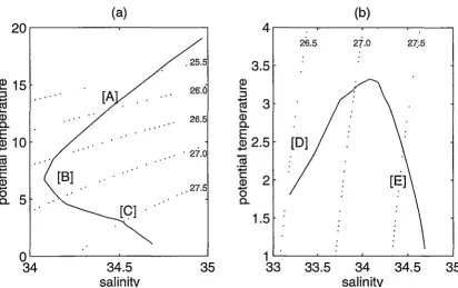
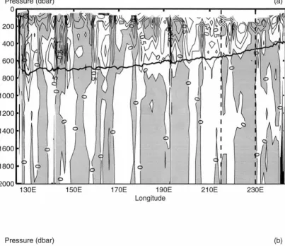
1 . Figure 2.2 illustrates Rpvarying through the water column.
~ 15
:::::;
~
Q)c..
ffi
10+-'
~
+:: c
Q)
0
c.. 5
(a)
[A
(b)
. 25.5 3.5
20.0
26.5
. 27.0
. 27.5
1.5
o~~~~~~~~~~~~ 1~~~~~~~~~
34 34.5
salinitv
35 33 33.5 34
salinitv
34.5 35
[image:24.569.110.523.393.652.2]2.4. The role of the stability ratio, Rp 19
In the central subtropical North Pacific below 100 dbar (Figure 2.2 a), temperature decreases monotonically with depth, giving aOz
>
0 throughout the water column. In region [A], which is in the main thermocline, salinity values decrease monotonically with depth (until a minimum is reached), giving f3Sz>
0. However, aOz»
f3Sz, consequently Rp>
1 in region [A]. On a conventional 0-S plot, where salinity is plotted against potential temperature, Rp>
1 is therefore the part of the 0-S curve with a positive slope. Region [B] is at the salinity minimum, which in this case represents North PacificIntermediate Water (NPIW). There, f3Sz = 0 and Rp = oo. In region [CJ, the 0-S curve has a negative slope. Salinity 'increases monotonically with depth to the bottom, giving f3Sz
<
0 and Rp<
0.In another example, in the western subarctic Pacific (Figure 2.2 b), salinity increases monotonically with depth from the surface, giving f3Sz
<
0 throughout the water column. The main thermocline is absent. Instead,temperature increases slightly to a maximum at about 500 dbar, then decreases monotonically with depth to the bottom. Therefore in region [D], aez
<
0, but because aez«
f3Sz, 0<
Rp<
1. Region [E] has the same 0-S structure as region [C], having Rp<
0.Within these three "well-defined" ranges, different signs of aO'ln and
aO'Jz (similarly for (3S'ln and (3S'Jz ), at various parts of the water column can be the manifestation of the same surface process. For example, waters in the main thermocline (Rp
>
1) that have undergone pure freshening will show a decrease in salinity both on isobars and on isopycnals, whereas waters in region [DJ in Figure 2.2 (0<
Rp<
1) will show freshening on isobars but salinity increase on isopycnals, under the same pure freshening process.2.5. Decomposing water mass changes into three components 20
Pure Warming Pure Cooling Pure Freshening Pure Salinification
all'lz > 0 aB'lz < 0 all'lz = 0 all'lz = 0
,BS'lz = 0 ,BS'lz = 0 ,BS'lz < 0 ,BS'lz > 0
1 < Rr < +oo ,BS'ln = all' In< 0 ,BS'ln = all' In> 0 ,BS'ln =all' In< 0 ,BS'ln =all' In> 0 -oo < Rr < 0 ,BS'ln =all' In> 0 ,BS'ln = all' In< 0 ,BS'ln = aB'ln < 0 ,BS'ln =all' In> 0
0 < Rr < 1 ,BS'ln = aB'ln > 0 ,BS'ln = aB'ln < 0 ,BS'ln =all' In> 0 ,BS'ln = aB'ln < 0
Table 2.1: The different signs of
aO'ln, ,BS'ln, aO'lz
and,BS'lz
for the two "pure" processes that involve water mass changes: (i) pure warming (cooling), and (ii) pure freshening (salinification), for various values of Rp.2.5
Decomposing water mass changes into
three components
Any observed changes in water mass characteristics can be decomposed into these three processes. This is done by setting up a linear system, using the three "pure" processes as a basis. Inverse methods are then applied to estimate the strength of each component.
Equations 2.7, 2.8 and 2.9 define the relations between the stability ratio
Rp and the six "observable" variables:
aO'ln, aO'lz, aN'Oz, ,BS'ln, ,BS'lz,
and,BN' Bz,
for each of the three "pure" processes. These are related to change in in-situ density by the Equation of State:p-
1p'lz
=
,BS'lz - aO'lz·
Let the three model parameters:p-
1p'lzAw, p-
1p'lzAf,
andp-
1p'lzAh,
be the relative strength of each process in causing the observed changes, then a linearnon-homogeneous system of the form Gm= d can be found, where the model parameters m =
p-
1p'lz ·[Aw, Af, Ah]
can be estimated, using inverse methods,2.5. Decomposing water mass changes into three components
negative values indicate pure freshening. Lastly, negative values of p-1
p'lz
Ah mean downward movement of isopycnals, i.e. density surfaces deepen in time.Appendix A details the setting up of the linear system Gm= d, for all values of Rp, except for when Rp = 1, where the system is undefined. In deriving this linear system, the first term of the Taylor's series expansion has been used to obtain
aO'ln - aO'lz
=
aN'Oz
and.BS'ln - .BS'lz
=
.BN' Bz
(see Equations 2.2 and 2.3). Hence our linear system is accurate to the first order.The model matrix G takes the form:
-(Rµ - 1) 0 -RP
1 Rµ 0
G 1 Rp Rp Rµ
Rµ-l 0 (Rp - 1) -1
1 Rµ 0
1 1 1
for the three "well-defined" ranges : 1
<
Rp<
+oo , -oo<
Rµ<
0 and21
0
<
Rp<
1. The three columns represent the effects of pure warming/ cooling, pure freshening/salinification and pure heaving respectively, on the sixobservable variables. The set of three vectors, comprised of the three columns, is not linearly independent. The set of six observable variables also is not
linearly independent. In fact, the rank (the number of linearly independent rows or columns in a matrix) of the matrix G is 2.
To solve the system Gm= d, each column of G is first normalised by its L2 norm to improve its condition number. This is done by forming a diagonal matrix of weights W, then forming a new weighted matrix G' = G W. The weighted matrix G' is consequently decomposed by singular value
decomposition: G' =
u
AVTw-
1. The eigenvalues, which are the diagonal elements in A, are either positive distinct or zero. A particular solution of the form:(2.10)
2.5. Decomposing water mass changes into three components 22
(i) solution to the under-determined problem
G, as mentioned previously, has rank equals 2, so the system Gm= d
with m having 3 model parameters: p-1p'\zAw, p-1p'\zAf and p-1p'\zAh, is
under-determined. If an under-determined system has at least one solution, then the solution set is infinite. Here, only the natural solution (Equation 2.10) is considered, with k = 2 , i.e. two eigenvalues are retained. In the
under-determined case, the natural solution is equivalent to the minimum length solution (Menke
(1984),
p.119), i.e. m~st · mest is minimized (theL
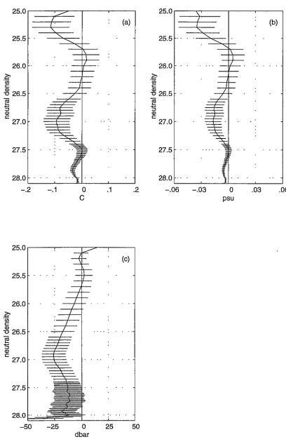
2 norm of the solution length is minimized). Solving Gm= d as an under-determined system has the effect of distributing the variance needed to explain the data between all three processes, thus revealing the relative strength of each process in causing the observed () and S changes. However, where the strengths of the signals are weak and noise dominates the observations (e.g. in deeper waters), this solution tends to distribute the variance equally between all three processes. Hence at those places, this solution should be used critically. 90% error bars are provided with this solution and should give an indication of the reliability of the solution.(ii)
solution to the over-determined problem
If it is assumed that only one process is present and that the other two processes are absent, then there is only one model parameter, and Gm = d
becomes an over-determined system. In this case, Equation 2.10 is used with k = 1, i.e. one eigenvalue is retained. In the over-determined case, the natural solution is equivalent to the least squares solution, where
[ d - G mestF · [ d - G mest] is minimized (the L2 norm of the prediction error is minimized). When solving for the single-process system, the percentage
variance explained by each single process is defined by
d~~--~st.
Solving Gm =d
as an over-determined system for each individual parameter has the advantage of showing which single process best explains the observations.(iii) solution to the evenly-determined problem: the
special cases of
B-S
extrema
At salinity minima and maxima, vertical salinity gradients Sz equal zero, so Rp = ±oo. Pure warming/cooling (Equation 2.7) simplifies to
aB'\z/ Rp
2.5. Decomposing water mass changes into three components 23
However,
aO'ln
=,BS'ln
= 0 is exactly the conditions for pure heaving. The subsurface changes as a result of pure warming/cooling and pure heaving therefore exhibit the same relations at salinity minima and maxima. In other words, at precisely Rp = ±oo , pure warming/ cooling and pure heaving collapse into a single process: AwII
Ah. The linear system degenerates into:-1 0
aO'lz
0 1
aO'ln
P-1P1
lz ·
1 1 . [Aw1~
A"l
aN'Oz
0 1
,BS'lz
0 1
,BS'ln
0 0
,BN'Sz
-1 0 0 1
The model matrix G
=
1 1 still has rank equal 2 in this degenerate case.0 1
0 1
0 0
This means that the two columns in G are linearly independent, and that the linear system Gm = d is now evenly-determined, with only two model
parameters: p-1
p'lz
(AwII
Ah) and p-1p'lz
Af.At temperature minima and maxima, vertical temperature gradients
Oz
equal zero, so Rp=
0. Pure freshening/salinification (Equation 2.8) simplifies toTherefore, pure freshening/salinification and pure heaving also collapse into a single process: Af
II
Ah, and in this case the linear system becomes:1 0
aO'lz
1 0
aO'ln
P-1P1
lz ·
0 0. [
Af~~A"
l
aN'Oz
0 -1
,BS'lz
1 0
,BS'ln
2.5. Decomposing water mass changes into three components
1 0
1 0
G= 0 0
0 -1 also has rank equal 2. Again there are only two model 1 0
1 1
parameters:
p-
1p'lzAw
andp-
1p'lz (Al
11Ah),
so Gm= dis alsoevenly-determined when Rp = 0.
24
Chapter
3
Observational data sets and
treatment of data
In this chapter, the observational data sets, and the interpolation
procedure that has been applied to the data, are presented. The observational data sets used can be classed into two groups. The first group is the collection of historical hydrographic data sampled before the 1980s. The second group is the set of modern hydrographic one-time transects that were sampled during the 1980s and 1990s under the World Ocean Circulation Experiment (WOCE). Decadal changes in the interior of the North and South Pacific oceans are examined by comparing these two groups of observational data. The ways in which the Bindoff and McDougall (1994) method (developed in Chapter 2) have been applied to the data are also explained.
3.1
Observational data sets
3.1.1
Historical hydrographic data sets
The main historical data set used in this thesis is the world data set compiled by J.L. Reid and A.W. Mantyla. The data set has been compiled over many years and from many sources, and has been used in various world ocean studies by the same authors. It is edited constantly as new data become available and some data are eliminated. Only stations that reach close to the bottom are included (pers. comm. with J. Reid). The version of the North and South Pacific historical data set used in this study was obtained in 1994 from an anonymous ftp site at Scripps Institute of Oceanography. This version contains 1332 hydrographic casts that span the years from 1929 to 1980 for the
3.1. Observational data sets
North Pacific, and 1778 hydrographic casts that span the years from 192_5 to 1980 for the South Pacific. The data set consists mainly of Nansen casts. Figure 3.1 shows the locations of these data points.
60N 40N 20N 0 208 408
608
.
.
.
.
.
.
.
.
.
·.:.
. . .
·.
.
.
..
:•.
.. : · .. :··:=·-i
.
:
:
.
:
.
.
.,.
. . . . ·= . .. :· ..
. .
.
. .
··.::
. . . .
,,,.
~:·..
. ·: ·i·:
··:::.·:.: ..
: ·~:
·:·:; ...
: r ..
~:r::
..
.
i .
~::
:
.
.
.
.
.
.. .
.
.
.
.
.
...
. .
·
.
t ... :· ·:·: .. ,: .....
. .
..
. .
.
.
.
..
.· .·
..
..
..
..
...
··. ·. . ·: =· ... ;
:..
.
::·
...
·-::·
t• • .•...
I • : ••..
·.
~.
.
.
·..
..: \.
. ...
'
.
.
.
:.. :.r:. . .
. .
.
.
. .... .
.... .
.
.
.
. .
...
·
.
.
.
...
. .
. . .
.·
-:-.
·.~·:·. .
:
::..
...
.
.
..
.
. .. .
.
-.
..
. .
.
.
.
.
.
·:·,·~...
:
·
..
·:·
...
:. ·
.. ·
.... .
.
. .
:
..
.
.. .
...
.
. . .
..
.
.·
. .
. .
·:·:.:
.·:.:·:. :·:....
: ···.~ · · : · ... : . \ 1 1 : . · •• • •• :.·:::·'· •.•. : i .i : : ·.;.·::.
-~
.
.. !··· .. ·:· ::\•:··:: ..
.
.
...
.
.
.
..
.
.
. . . . · .. : . : . I· : . . : : .
:=·· .
.
.. · ..
~::·
26
808'--~~~~~~--'---"'=--~~~--'..._::=...~~~~~-'-~~~----'""---='--'
100E 150E 200E 250E 300E
Figure 3.1: The locations of the data points in the Reid and Mantyla Pacific data set.
3.1. Observational data sets 27
"Hydrographic Atlas of the Southern Ocean" by Olbers et al. (1992). Both of these atlases contain more Southern Ocean data points than the Reid and Mantyla world data set. The Olbers et al. (1992) atlas includes German and Russian data and so has a greater data density than the Gordon et al. (1982) atlas. It is for this reason that the Olbers et al. (1992) atlas data set is chosen as our historical hydrographic data set for the part of the South Pacific south of 30°S.
The Olbers atlas data set contains both Nansen and CTD casts. Each cast has been interpolated onto 42 standard depth levels. Harris (1996) performed further data quality tests on this data set and reduced the number of "clean casts" from 38818 to 23806. This thesis utilises the set of 23806 Olbers "clean casts" as described in Harris (1996). Figure 3.2 shows the locations of the
"clean casts" between longitudes 100°E and 300°E .
...
.
208 \\" I
o"
.
·
...'
.
I·-
.
.
,•..
•'
.
..
,
.:~-J-=:!
'I: · -
. ..
BQSL-~~~~~~_i_____s:;=-~~~~~-=--~~~~~--1~~~~~---==----i
100E 150E 200E 250E 300E
3.1. Observational data sets. 28
3.1.2
Modern WOCE transects
WOCE, the World Ocean Circulation Experiment, is a project of the World Climate Research Programme. Its goal is to collect high quality data sets of the global ocean, so that a comprehensive description of the global ocean and its circulation can be established. The data are also ,intended for use with numerical models, so that the ability of numerical models for climate prediction can be improved. During the 1980s and the 1990s, many intensive one-time hydrographic surveys were carried out in the Pacific Ocean. By 1997, at the time of writing of this thesis, six trans-Pacific one-time hydrographic surveys were available from the WOCE Hydrographic Program publicly available data archive, accessible via an anonymous ftp site at nemo.ucsd.edu (the North American mirror site). These six1 publicly available WOCE Pacific transects are Pl, P3, P4, P6, P16 and Pl 7 ..
Of these six surveys, four are used in this thesis because they lie in areas with sufficient historical data for the purpose of comparison. These four WOCE sections are Pl, P3, P4 and P16. P6, the zonal transect that occupies the nominal latitude of 32.5°8, lies in a historically data sparse area, and is therefore deemed not suitable for the purpose of this study. P16 and Pl 7 are two meridional transects that lie close to each other, occupying the nominal , longitudes of 150.5°W and 135°W respectively. P16 was chosen over Pl 7 because of the slightly more abundant historical data distribution around it.
In addition to the above four publicly available transects, another more recently completed WOCE Pacific hydrographic surveys has been provided by the principal investigator for use in this study. This is P21 (preliminary data), provided by Dr. Harry Bryden of Southampton Oceanography Centre.
Together, these five transects form a set of modern Pacific data for comparison against the historical data.
Figure 3.3 shows the cruise tracks of these five transects. Table 3.1 lists the sampling dates, the nominal positions, and the chief scientists for these cruises.
1 Along P19, only the short Antarctic section, P19A, which runs from 70°8 to 67.5°8 along
3.1. Observational data sets 29
60N
40N
---~----~
20N
-
...
P4
0 P16C
.·
... P21"
208
..
P16 S
408
'd
1.
P16A608
.
100E 150E 200E 250E 300E
3.2. Treatment of data 30
Transect Sampling dates Nominal Chief scientist position
Pl 5 Aug to 7 Sep 1985 47°N L.Talley
'
P3 30 Mar to 3 Jun 1985 24°N J .Swift/D.Roemmich
P4 9 Feb to 10 May 1989 9.5°N J.Toole/E.Brady/H.Bryden
P16 S 11 Aug to 25 Aug 1991 150.5°W J.Swift P16 C 1 Sep to 30 Sep 1991 155°W L.Talley P16 A 12 Oct to 28 Oct 1992 150.5°W J.Reid
P21 27 Mar to 25 Jun 1994 17.5°8 M.McCartney /H.Bryden Table 3.1: The sampling dates, nominal positions, and chief scientists for the seven WOCE Pacific transects used in this thesis.
3.2
Treatment of data
To compare the two sets of data: the modern WOCE set and the historical set, some interpolations need to be done so that the data points occupy common coordinates, vertically and laterally. This section details the interpolation procedures in the order that have been applied to the data. Then the calculations for obtaining'the variables needed in the diagnostic method are described.
3.2.1
Vertically interpolating to neutral surfaces
3.2. Treatment of data 31
subsampled at these 38 standard pressures, by averaging 10 dbar above and below each level. All historical in-situ temperature and salinity data have also been linearly interpolated to this set of 38 standard pressures, except for data from the Olbers atlas, which have already been interpolated onto a similar set of 42 standard depths (m) during the production of the atlas.
II
LevelI
PressureII
LevelI
PressureII
LevelI
PressureII
LevelI
PressureII
1 0 11 400 21 1400 31 3750
2 10 12 500 22 1500 32 4000
3 20 13 600 23 1750 33 4250
4 50 14 700 24 2000 34 4500
5 75 15 800 25 2250 35 4750
6 100 16 900 26 2500 36 5000
7 150 17 1000 27 2750 37 5500
8 200 18 1100 28 3000 38 6000
9 250 19 1200 29 3250
10 300 20 1300 30 3500
Table 3.2: The 38 standard pressures (dbar) that are chosen to imitate an average Nansen cast. All WOCE CTD casts have been subsampled at these pressures, and all Reid and Mantyla historical data points have been linearly interpolated to these levels.
In-situ temperature and salinity on these 38 standard pressures (or the 42 standard depths for the Olbers atlas data), from the historical data and the WOCE data, are then labelled with neutral densities (Jackett and McDougall 1995; Jackett and McDougall 1997). Neutral density '"'In (in kg m-3) is preferred to potential density because the ambiguity associated with choosing reference pressures for potential density is eliminated. A set of '"'In surfaces is subsequently selected. Quadratic interpolation then provides in-situ temperature, salinity and pressure (and therefore potential temperature) on these specific '"'In surfaces, for every data point. In this manner, all historical casts and all modern WOCE CTD casts are vertically interpolated to a set of common neutral density coordinates.