A Cartesian-grid integrated-RBF Galerkin technique

D. Ho-Minh1, N. Mai-Duy1and T. Tran-Cong1

Abstract: This paper describes a high-order Galerkin technique, which is based on indirect/integrated radial-basis-function networks (IRBFNs) and Cartesian grids, for the discretisation of elliptic problems in two dimensions. The field variable is approximated by high-order IRBFNs that can work on uniform grids without suffering from Runge’s phenomenon. Unlike conventional Galerkin techniques, derivative boundary values are incorporated into the approximations and their imposition is conducted in an exact manner. The Galerkin formulation is then applied to force IRBFNs to satisfy the governing equation. The present technique is verified numerically through the solution natural convection in a square slot - a benchmark problem in CFD. Highly accurate solutions are obtained using relatively coarse grids, which show the effectiveness of using RBFs as trial functions in the Galerkin formulation.

Keywords: Integrated RBFNs, Galerkin approach, Cartesian grids, elliptic problems.

1 Introduction

Radial-basis-function networks (RBFNs) have been shown to be a powerful numerical tool for the solution of partial-differential equations (PDEs). The first report on this subject was made by Kansa (1990). For Kansa’s method, a function is first represented by an RBFN which is then differentiated to obtain approximate expressions for its derivative functions. On the other hand, to avoid the reduction in convergence rate caused by differentiation, Mai-Duy and Tran-Cong (2001) proposed an indirect/integrated RBFN (IRBFN) approach in which the highest-order derivatives in the PDE are first decomposed into RBFs, and their lower-order derivatives and the function itself are then obtained through integration. Previous studies (e.g. [Mai-Duy and Tran-Cong (2001)]) showed that IRBFN collocation methods yield better accuracy than differentiated RBFN (DRBFN) ones for both the representation of functions and the solution of PDEs.

Since the global RBF interpolation matrix is fully populated and its condition number grows rapidly with respect to the increase of RBF centres and/or widths [Schaback (1995)], several RBF techniques based on local approximations have been proposed. In the context of IRBFNs, colloca-tion schemes, based on one-dimensional (1D) IRBFNs and Cartesian grids, for the solucolloca-tion of 2D

1_{Computational Engineering and Science Research Centre (CESRC), Faculty of Engineering and Surveying (FoES),}

elliptic PDEs were reported in, e.g. [Mai-Duy and Tran-Cong (2007)]. The RBF approximations at a grid node involve only points that lie on the grid lines intersected at that point rather than the whole set of nodes. As a result, the construction process is conducted for a series of small matrices rather than for a large single matrix (“local” approximation).

Along with the point-collocation approach, a Galerkin-type approach, based on 1D-IRBFNs, has been developed in [Mai-Duy and Tran-Cong (2009)]. In this approach, the boundary conditions are satisfied in a local sense using the point collocation formulation, and the solution to the problem is satisfied in a global sense using the Galerkin formulation. The use of integration to construct the approximations generates some additional coefficients (i.e. the constants of integration) that can be exploited for the effective implementation of Neumann and multiple boundary conditions. The resultant system of algebraic equations is often symmetric and has a relatively-low condition number, which facilitate the employment of much larger numbers of nodes. Numerical results showed that this technique yields accurate results, high rates of convergence, and especially similar levels of accuracy for both types of problems(i.e. Dirichlet only and Dirichlet-Neumann boundary conditions).

In this paper, the high-order Galerkin technique, which is based on 1D-IRBFNs and Cartesian grids, is applied to simulate natural convection in a square slot. It will be shown that convergent solutions are achieved for very high values of the Rayleigh number (i.e. up to 108). Numerical results obtained are compared with those by other techniques available in the literature.

The remainder of this paper is organised as follows. Section 2 presents the proposed integrated-RBF Galerkin method, including the Galerkin formulation, 1D-Iintegrated-RBFN representations of the field variables and imposition of boundary conditions. A CFD benchmark test problem is simulated in section 3. Section 4 concludes the paper.

2 The integrated-RBF Galerkin technique

2.1 Galerkin formulation

Let

u(x) =

N

∑

αiφi(x)_≈u¯(x), (1)

be an approximate solution to a differential equation of the form

L(u¯) = 0 x_∈Ω, (2)

with its boundary conditions of the form

In Eq. 1, Eq. 2 and Eq. 3, u is the field/dependent variable, the overbar denotes the exact solution,

L the prescribed differential operator, Ωthe problem domain,Γ the boundary of the domainΩ,

{αi}Ni=1 the set of unknown coefficients and{φi(x)} N

i=1the set of linearly-independent functions. The termsφi are usually referred to as the trial/basis/approximating functions.

The unknown coefficientsαican then be found by constructing a scheme to minimise the following residuals

Rs=L(u) (4)

and

Rb=B(u). (5)

This process can be stated mathematically as

Z

ΩW RsdΩ+

Z

ΓW Re bdΓ=0 (6)

where W and W are weighting functions to be chosen. The Galerkin formulation chooses thee

weighting function from the set of trial functions, i.e. W(x) =φi(x). The above volume integrals can be evaluated numerically using Gaussian quadrature.

2.2 One-dimensional IRBFN representations of the field variables

In this work, the system of PDEs is of second order. Consider a x grid line. Applying the integral RBF scheme of second order, a function f and its derivatives with respect to x can be represented as follows

d2f(x)

dx2 =

Nx

∑

wigi(x) = Nx

∑

wiIi(2)(x), (7)

d f(x)

dx =

Nx

∑

wiIi(1)(x) +c1, (8)

f(x) =

Nx

∑

wiIi(0)(x) +c1x+c2, (9)

where Nx is the number of nodes on the grid line, {wi}N_i=1x the set of network weights, and

{gi(x)}N_i=1x ≡ n

I_i(2)(x)oNx

i=1 the set of RBFs, I (1) i (x) =

R

Evaluation of Eq. 7 - Eq. 9 at the grid nodes leads to

d

d2_f

dx2 = Ib

(2)_{αb, (10)}

c

d f

dx = Ib

(1)_{αb, (11)}

b

f = Ib(0)α_{b, (12)}

where the superscript(.)is used to denote the order of the corresponding derivative function;

b

I(2) ₌

     

I₁(2)(x1), I2(2)(x1), · · ·, IN(2)x (x1), 0, 0 I₁(2)(x2), I2(2)(x2), · · ·, IN(2)x (x2), 0, 0

..

. ... . .. ... ... ...

I₁(2)(xNx), I

(2)

2 (xNx), · · ·, I

(2)

Nx (xNx), 0, 0

     ; b

I(1) ₌

     

I₁(1)(x1), I2(1)(x1), · · ·, IN(1)x (x1), 1, 0 I₁(1)(x2), I2(1)(x2), · · ·, IN(1)x (x2), 1, 0

..

. ... . .. ... ... ...

I₁(1)(xNx), I

(1)

2 (xNx), · · ·, I

(1)

Nx (xNx), 1, 0

     ; b

I(0) ₌

     

I₁(0)(x1), I2(0)(x1), · · ·, IN(0)x (x1), x1, 1 I₁(0)(x2), I2(0)(x2), · · ·, IN(0)x (x2), x2, 1

..

. ... . .. ... ... ...

I₁(0)(xNx), I

(0)

2 (xNx), · · ·, I

(0)

Nx (xNx), xNx, 1

     ; b

α = (w1,w2,· · ·,wNx,c1,c2)

T_;

and

d

dk_f

dxk =

dkf1

dxk ,

dkf2

dxk ,· · ·,

dkfNx dxk

T

, k=_{1,2_},

b

f = (f1,f2,· · ·,fNx)

T

,

in which dkfj

dxk=dkf(xj)

The relations between the RBF-coefficient spaceαb and the physical space bf are given by _b f b e = " b I(0) c K # b

α =Cbα_{b, (13)}

b

α = Cb−1

_b f b e , (14)

where _be=Kcα_{b represents the extra information (e.g. normal derivative values at the two}

end-points) andCb_{the conversion matrix.}

Making use of Eq. 14, the values of f and its derivatives at an arbitrary point x on the grid line will be computed by

f(x) = I₁(0)(x),I₂(0)(x),_···,I_N(0)

x (x),x,1

b

C−1

_b f b e , (15)

∂f(x)

∂x =

I₁(1)(x),I₂(1)(x),_···,I_N(1)

x (x),1,0

b

C−1

_b f b e , (16)

∂2_f(x)

∂x2 =

I₁(2)(x),I₂(2)(x),_···,I_N(2)_x (x),0,0

b

C−1

_b f b e . (17)

They can be rewritten in compact form

f(x) =

Nx

∑

ϕi(x)fi+ϕNx+1(x)e1+ϕNx+2(x)e2, (18)

∂f(x)

∂x =

Nx

∑

∂ϕi(x)

∂x fi+

∂ϕNx+1(x)

∂x e1+

∂ϕNx+2(x)

∂x e2, (19)

∂2_f(x)

∂x2 =

Nx

∑

∂2ϕi_(x) ∂x2 fi+

∂2ϕN

x+1(x)

∂x2 e1+ ∂2ϕN

x+2(x)

∂x2 e2, (20)

where_{ϕi_}Nx+2

i=1 is the set of IRBFN basis functions in the physical space.

One can take products of integrated RBFs in each direction as basis functions for the interpolation of f over the entire 2D domain. The IRBFN approximation is defined everywhere in the domain. It is easy to get the value of f at any point in the domain.

2.3 Imposition on boundary conditions

If PDEs are subject to Dirichlet boundary conditions only, the matrixKc_{and the vectore in Eq. 13b}

In the case of Cartesian coordinate system, approximate expressions for the field variable u will take the form

u(x,y) =

Nx

∑

Ny

∑

ϕ(x) i (x)ϕ

(y)

j (y)ui,j, (21)

where Nxand Nyare the numbers of grid lines in the x and y directions, respectively.

Consider PDE subjecting to both types of boundary conditions. Assume that Dirichlet and Neu-mann boundary conditions are prescribed on the two vertical and two horizontal walls, respec-tively. The integral approach allows one to incorporate Neumann boundary conditions into the IRBFN approximations through the integration constants. For each y grid line, the matrixKc_and

the vector_be in Eq. 13 will become

c

K ₌

"

I₁(1)(y1), I₂(1)(y1), ···, I_N(1)_y (y1), 1, 0

I₁(1) yNy

, I₂(1) yNy

, _···, I_N(1) y yNy

, 1, 0

#

,

b

e =

∂u1

∂y

∂uNy ∂y

!

,

leading to

u(x,y) =

Nx

∑

ϕ(x) i (x)

Ny

∑

ϕ(y)

j (y)ui,j+ϕN(y)y+1(y)

∂ui,1 ∂y +ϕ

(y) Ny+2(y)

∂ui,Ny

∂y

!

. (22)

In Eq. 21 - Eq. 22, ui,jis the values of the u variable at the intersection of the ith horizontal grid line and jth vertical grid line; the productsϕ_i(x)ϕ(y)_j are usually referred to as the trial/basis/approximating functions; and∂ui,1

∂y and∂ui,Ny

∂y are nodal boundary derivative values.

3 Application of the proposed technique

Simulation of natural convection in a square slot is conducted here to further validate the proposed technique. For this benchmark test problem, uniform grids are used to represent the computational domain, and 1D-IRBFNs are implemented with the multiquadric (MQ) function

gi(x) = q

(x₋ci)2+a2i,

3.1 Problem definition

The governing equations which are obtained from the streamfunction-vorticity-temperature for-mulation can be written as

∂2ψ ∂x2 +

∂2ψ

∂y2 = −ω, (23)

∂ω ∂t +u

∂ω ∂x +v

∂ω

∂y =

r

Pr Ra

_∂2ω ∂x2 +

∂2ω ∂y2

+∂T

∂x, (24)

∂T

∂t +u

∂T

∂x +v

∂T

∂y =

1

√ RaPr

_∂2

T

∂x2 + ∂2_T

∂y2

, (25)

where

u=∂ψ

∂y, v=−

∂ψ ∂x,

In Eq. 25 , Pr and Ra are the Prandtl and Rayleigh numbers defined as Pr =ν/α and Ra=

βg∆T L3αν_{, respectively in which}ν _{is the kinematic viscosity,}α _{the thermal diffusivity,}β _the thermal expansion coefficient, g the gravity, and L and∆T the characteristic length and temperature

difference, respectively. In this dimensionless scheme, the velocity scale is taken as U=pgLβ∆T

for the purpose of balancing the buoyancy and inertial forces.

The domain of interest is an enclosed square slot with all stationary walls, leading toψ=∂ψ/∂n=

0 on the boundaries. The two horizontal walls are adiabatic (i.e. ∂T/∂y=0), while the two ver-tical walls are maintained at constant temperatures (i.e. T = +0.5 (left wall) and T=₋0.5 (right wall)).

3.2 Computation boundary conditions for the vorticity

The computation boundary conditions for the vorticity can be derived from the streamfunction equation. The process is similar to that in [Ho-Minh, Mai-Duy, and Tran-Cong (2009)].

Taking into account the streamfunction boundary values (i.e.ψ=0), expressions for the vorticity on the boundaries will reduce to

ω=∂

2ψ

∂n2, (26)

where n is the local direction normal to the wall.

Consider a x grid line. Owing to the fact that the present coefficient vector is larger, one can add two extra equations representing∂ψ1/∂x and∂ψNx/∂x to the conversion process

   b ψ ∂ψ1 ∂x ∂ψNx ∂x   = " b I(0) c K # b

in whichKc_{is the matrix made up of the first and last rows of}Ib(1)_{, i.e.}

c

K ₌

"

I₁(1)(x1), I₂(1)(x1), ···, I_N(1)_x (x1), 1, 0

I₁(1)(xNx), I

(1)

2 (xNx), ···, I

(1)

Nx (xNx), 1, 0

#

.

It can be seen from Eq. 27 that, despite the presence of nodal derivative values, the approximate solutionψis collocated at the whole set of centres on the grid line.

The second derivatives of ψ at the two boundary points can now be expressed in terms of the values ofψ at every point on the grid line and the values of∂ψ∂x at the two boundary points (x1,xNx)

∂2_ψ 1

∂x2

∂2_ψ Nx ∂x2

!

=DbCb−1

  

b ψ

∂ψ1

∂x

∂ψNx ∂x

 

, (28)

whereDb_{is the sub-matrix of}Ib(2)_{(i.e. the first and last rows)}

b

D₌

"

I₁(2)(x1), I2(2)(x1), ···, IN(2)(x1), 0, 0

I₁(2)(xNx), I

(2)

2 (xNx), ···, I

(2)

N (xNx), 0, 0

#

,

andCb_{is defined in Eq. 27.}

It can be seen that the IRBFN approximations for∂2ψ∂x2 at the boundaries satisfy exactly the prescribed derivative boundary values. With Eq. 28, we can obtain the computational boundary conditions for the vorticity. On a y grid line, the process can be taken in a similar fashion.

3.3 Solution procedure

Using the 1D-IRBFN scheme introduced in section 2.2 and 2.3, the approximation of ψ,ω is taken the form of Eq. 21. Because the energy equation Eq. 25 is subject to both types of boundary conditions, the variable T can be approximated by Eq. 22.

1. Guess values of T ,ψ,ω and their first-order spatial derivatives at time t=0

2. Discretise spatial derivatives using 1D-IRBFNs, resulting in a high-order approximation scheme in space

3. Discretise time derivatives using Euler (forward difference) method, resulting in a first-order accurate scheme in time

4. Compute the convective terms and the boundary values for ω with the process given in section 3.2

5. Solve the energy equation Eq. 25 for T , subject to Dirichlet and Neumann conditions Solve the vorticity equation Eq. 24 forω, subject to Dirichlet conditions

Solve the streamfunction equation Eq. 23 forψ, subject to Dirichlet conditions

6. Check to see whether the solution has reached a steady state r

∑N i=1

T_i(k)₋T_i(k−1)2

r ∑N

i=1

T_i(k)

2 <ε, (29)

where k is the time level andεis a prescribed tolerance

7. If it is not satisfied, advance time step and repeat from step 3. Otherwise, stop the computa-tion and output the results.

3.4 Results and discussion

Numerical results for this problem are extensive. A range of Ra from 103to 106has been widely used for the validation of new numerical schemes. Davis (1983) provided finite-difference results which have been then often cited in the literature for comparison purposes. Later on, there are increased levels of interest for higher values of Ra, namely 107 and 108. Works reported include [Quéré (1991)] (the pseudo-spectral method), [Wan, Patnail, and Wei (2001)] (FEM), [Wan, Pat-nail, and Wei (2001)] (discrete singular convolution (DSC) method), [Sadat and Couturier (2000)] (meshless diffuse approximation method (DAM)), and [Kosec and Sarler (2007)] (mesh-free local RBF collocation method (RBFCM)). For this higher range, it has been generally observed that (i) the strength of boundary layers is significantly increased, (ii) convergence becomes much more difficult, and (iii) significant discrepancies in the Nusselt number occur in some cases (e.g. be-tween the pseudo-spectral technique [Quéré (1991)] and the DSC method [Wan, Patnail, and Wei (2001)]).

• The average Nusselt number on the vertical plane at x=1/2 (middle cross-section), which is defined by

Nu1_/2 = Nu(x=1/2,y),

in which

Nu(x,y) =

Z 1

0

uT₋∂T

∂x

dy. (30)

• The average Nusselt number throughout the cavity, which is defined by

Nu =

Z 1

0

Nu(x,y)dx. (31)

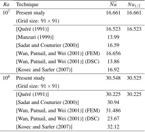
It is noted that integrals Eq. 30 and Eq. 31 are computed here using Simpson’s rule. Results for Ra from 107 to 108 are presented in Tab. 1 and Fig. 1. Tab. 1 shows a comparison of the average Nusselt numbers between the present method and several other methods. It can be seen that there are significant discrepancies among various numerical techniques. For the case of Ra=

107, the DSC [Wan, Patnail, and Wei (2001)] and FEM [Manzari (1999)] produced the values of 13.86 and 13.99 for the average Nusselt number, while the pseudo-spectral [Quéré (1991)], FE [Wan, Patnail, and Wei (2001)], DA [Sadat and Couturier (2000)] and RBFCM [Kosec and Sarler (2007)] techniques yielded the following values: 16.523, 16.656, 16.59 and 16.92. The differences between the two groups are much wider for the case of Ra=108: 23.67 for the DSC method, and (30.225, 31.486, 30.94, 32.12) for the second group. The Galerkin-IRBFN results are in close agreement with the second group, particularly with the pseudo-spectral technique [Quéré (1991)]. Variations of the local Nusselt number on the left and right walls are presented in Fig. 2. It is clearly shown that the proposed technique is able to capture very stiff changes of the local Nusselt number in the region close to the boundary. It can be seen from Fig. 1, the present contour plots for the streamfunction, vorticity and temperature variables look feasible when compared with those of the pseudo-spectral technique [Quéré (1991)]. Very thin boundary layers are formed at these high values of Ra. It is noted that iso-values used in these plots are the same as those used in [Quéré (1991)].

4 Concluding remarks

Table 1: Natural convection flow in a square slot: Comparison of the Galerkin-IRBFN results with those of other techniques at Ra=107and Ra=108(Pr=0.71)

Ra Technique Nu Nu1/2

107 _{Present study 16.661 16.661}

(Grid size: 91_×91)

[Quéré (1991)] 16.523 16.523

[Manzari (1999)] 13.99

[Sadat and Couturier (2000)] 16.59

[Wan, Patnail, and Wei (2001)] (FEM) 16.656 [Wan, Patnail, and Wei (2001)] (DSC) 13.86 [Kosec and Sarler (2007)] 16.92

108 Present study 30.548 30.525

(Grid size: 91_×91)

[Quéré (1991)] 30.225 30.225

[Sadat and Couturier (2000)] 30.94

[Wan, Patnail, and Wei (2001)] (FEM) 31.486 [Wan, Patnail, and Wei (2001)] (DSC) 23.67

Ra=107 _Ra=108

Streamlines Streamlines

Iso-vorticity lines Iso-vorticity lines

Isotherms Isotherms

Figure 1: Natural convection flow in a square slot: Contour plots for theψ,ω and T variables at

Left wall Right wall

0 20 40 60 80 100

0 0.1 0.2 0.3 0.4 0.5 0.6 0.7 0.8 0.9 1

Nusselt number (Nu)

y−coordinate

← Ra=10 8 ← Ra=10 7

0 20 40 60 80 100

0 0.1 0.2 0.3 0.4 0.5 0.6 0.7 0.8 0.9 1

Nusselt number (Nu)

y−coordinate

← Ra=108 ← Ra=107

Figure 2: Natural convection flow in a square slot: Variations of the local Nusselt number along the left and right walls.

of the Neumann boundary condition, and (iv) ability to capture very thin boundary layers using relatively-coarse grids.

Acknowledgement: This research is supported by Australia Research Council. D. Ho-Minh would like to thank the CESRC, FoES and USQ for a postgraduate scholarship.

References

Davis, G. D. V. (1983): Natural convection of air in a square cavity: a bench mark numerical solution. International Journal of Numerical Method Fluids, vol. 3, pp. 249–264.

Ho-Minh, D.; Mai-Duy, N.; Tran-Cong, T. (2009): A Galerkin-RBF approach for the streamfunction-vorticity-temperature formulation of natural convection in 2D enclosured domains.

CMES, vol. 44, pp. 219–248.

Kansa, E. J. (1990): Multiquadrics - A scattered data approximation scheme with applica-tions to computational fluid dynamics I. Surface approximaapplica-tions and partial derivative estimates.

Kosec, G.; Sarler, B. (2007): Solution of thermo-fluid problems by collocation with local pressure correction. International Journal of Numerical Methods for Heat and Fluid Flow, vol. 18, pp. 868–882.

Mai-Duy, N.; Tran-Cong, T. (2001): Numerical solution of differential equations using multi-quadric radial basis function networks. Neural Networks, vol. 14, pp. 185–199.

Mai-Duy, N.; Tran-Cong, T. (2007): A Cartesian-grid collocation method based on radial basis function networks for solving PDEs in irregular domains. Numerical Methods for Partial

Differential Equations, vol. 23, pp. 1192–1210.

Mai-Duy, N.; Tran-Cong, T. (2009): An integrated-RBF technique based on Galerkin formula-tion for elliptic differential equaformula-tion. Engineering Analysis with Boundary Elements, vol. 33, pp. 191–199.

Manzari, M. T. (1999): An explicit finite element algorithm for convective heat transfer prob-lems. International Journal of Numerical Methods for Heat and Fluid Flow, vol. 9, pp. 860–877.

Quéré, P. L. (1991): Accuracy solutions to the square thermally driven cavity at high Rayleigh number. Computers and Fluids, vol. 20, pp. 29–41.

Sadat, H.; Couturier, S. (2000): Performance and accuracy of meshless method for laminar natural convection. Numerical Heat Transfer, Part B, vol. 37, pp. 455–467.

Schaback, R. (1995): Error estimates and condition numbers for radial basis function interpola-tion. Advances in Computational Mathematics, vol. 3, pp. 251–264.