C
2011. The American Astronomical Society. All rights reserved. Printed in the U.S.A.
ARCHITECTURE AND DYNAMICS OF
KEPLER’S CANDIDATE MULTIPLE TRANSITING PLANET SYSTEMS
Jack J. Lissauer1, Darin Ragozzine2, Daniel C. Fabrycky3,14, Jason H. Steffen4, Eric B. Ford5, Jon M. Jenkins1,6, Avi Shporer7,8, Matthew J. Holman2, Jason F. Rowe6, Elisa V. Quintana6, Natalie M. Batalha9, William J. Borucki1,
Stephen T. Bryson1, Douglas A. Caldwell6, Joshua A. Carter2,14, David Ciardi10, Edward W. Dunham11, Jonathan J. Fortney3, Thomas N. Gautier, III12, Steve B. Howell1, David G. Koch1, David W. Latham3,
Geoffrey W. Marcy13, Robert C. Morehead6, and Dimitar Sasselov2 1NASA Ames Research Center, Moffett Field, CA 94035, USA;[email protected]
2Harvard-Smithsonian Center for Astrophysics, Cambridge, MA 02138, USA
3Department of Astronomy & Astrophysics, University of California, Santa Cruz, CA 95064, USA 4Fermilab Center for Particle Astrophysics, Batavia, IL 60510, USA
5211 Bryant Space Science Center, University of Florida, Gainesville, FL 32611, USA 6SETI Institute/NASA Ames Research Center, Moffett Field, CA 94035, USA 7Las Cumbres Observatory Global Telescope Network, Santa Barbara, CA 93117, USA 8Department of Physics, Broida Hall, University of California, Santa Barbara, CA 93106, USA
9Department of Physics and Astronomy, San Jose State University, San Jose, CA 95192, USA 10Exoplanet Science Institute/Caltech, Pasadena, CA 91125, USA
11Lowell Observatory, Flagstaff, AZ 86001, USA
12Jet Propulsion Laboratory, California Institute of Technology, Pasadena, CA 91109, USA 13Astronomy Department, University of California, Berkeley, CA 94720, USA
Received 2011 February 24; accepted 2011 July 20; published 2011 October 13
ABSTRACT
About one-third of the ∼1200 transiting planet candidates detected in the first four months of Keplerdata are
members of multiple candidate systems. There are 115 target stars with two candidate transiting planets, 45 with three, 8 with four, and 1 each with five and six. We characterize the dynamical properties of these candidate multi-planet systems. The distribution of observed period ratios shows that the vast majority of candidate pairs are neither in nor near low-order mean-motion resonances. Nonetheless, there are small but statistically significant excesses of candidate pairs both in resonance and spaced slightly too far apart to be in resonance, particularly near the 2:1 resonance. We find that virtually all candidate systems are stable, as tested by numerical integrations that assume a nominal mass–radius relationship. Several considerations strongly suggest that the vast majority of these multi-candidate systems are true planetary systems. Using the observed multiplicity frequencies, we find that a single population of planetary systems that matches the higher multiplicities underpredicts the number of singly transiting systems. We provide constraints on the true multiplicity and mutual inclination distribution of the multi-candidate systems, revealing a population of systems with multiple super-Earth-size and Neptune-size planets with low to moderate mutual inclinations.
Key words: celestial mechanics – planets and satellites: dynamical evolution and stability – planets and satellites: fundamental parameters – planets and satellites: general – planetary systems
Online-only material:color figures
1. INTRODUCTION
Kepleris a 0.95 m aperture space telescope that uses transit photometry to determine the frequency and characteristics of
planets and planetary systems (Borucki et al.2010; Koch et al.
2010; Jenkins et al.2010; Caldwell et al.2010). The focus of
this NASA Discovery mission’s design was to search for small
planets in the habitable zone, butKepler’s ultra-precise,
long-duration photometry is also ideal for detecting systems with
multiple transiting planets. Borucki et al. (2011a) presented five
Keplertargets with multiple transiting planet candidates, and these candidate planetary systems were analyzed by Steffen
et al. (2010). A system of three planets (Kepler-9=KOI-377;
Holman et al. 2010; Torres et al. 2011) was then reported,
in which a near-resonant effect on the transit times allowed Keplerdata to confirm two of the planets and characterize the dynamics of the system. A compact system of six transiting
planets (Kepler-11; Lissauer et al.2011), five of which were
confirmed by their mutual gravitational interactions exhibited
14Hubble Fellow.
through transit-timing variations (TTVs), has also been reported. These systems provide important data for understanding the dynamics, formation, and evolution of planetary systems (Koch
et al.1996; Agol et al.2005; Holman & Murray2005; Fabrycky
2009; Holman2010; Ragozzine & Holman2010).
A catalog of 1235 candidate planets evident in the first four
and a half months of Kepler data is presented in Borucki
et al. (2011b, henceforth B11). Our analysis is based on the
data presented by B11, apart from the following modifications: five candidates identified as very likely false positives by
Howard et al. (2011), Kepler Objects of Interest (KOIs) 1187.01,
1227.01, 1387.01, 1391.01, and 1465.01, are removed from the
list. The radius of KOI-1426.03 is reduced from 35R⊕to 13R⊕
(Section4). B11 reported that KOI-730.03’s period was almost
identical to that of KOI-730.02, putting these two planets in the 1:1 resonance. Upon more careful light-curve fits, we disfavor the co-orbital period of KOI-730.03 near 10 days as an alias. The period of KOI-730.03 is therefore increased to 19.72175
and its radius increased to 2.4R⊕. We do not consider the 18
candidates with estimated radiiRp > 22.4 R⊕. None of the removed candidates is in a multi-candidate system, but both of the candidates with adjusted parameters are. We are left with a total of 1199 planetary candidates, 408 of which are in multiple candidate systems, around 961 target stars.
B11 also summarizes the observational data and follow-up programs being conducted to confirm and characterize planetary candidates. Each object in this catalog is assigned a vetting flag (reliability score), with 1 signifying a confirmed or validated
planet (>98% confidence), 2 being a strong candidate (>80%
confidence), 3 being a somewhat weaker candidate (>60%
confidence), and 4 signifying a candidate that has not received ground-based follow-up (this sample also has an expected
reliability of>60%). For most of the remainder of the paper, we
refer to all of these objects as “planets,” although 99% remain unvalidated and thus should more properly be termed “planet candidates.” Ragozzine & Holman (2010), Lissauer et al. (2011),
and Latham et al. (2011) point out that KOIs of target stars
with multiple planet candidates are less likely to be caused by astrophysical false positives than are KOIs of stars with single candidates, although the possibility that one of the candidate signals is due to, e.g., a background eclipsing binary, can be non-negligible.
The apparently single systems reported by B11 are likely to include many systems that possess additional planets that have thus far escaped detection by being too small, too long period, or too highly inclined with respect to the line of sight.
Ford et al. (2011) discuss candidates exhibiting TTVs that may
be caused by these transiting planets, but so far no
non-transiting planets have been identified. Latham et al. (2011)
compare various orbital and physical properties of planets in single candidate systems to those of planets in multi-candidate
systems. We examine herein the dynamical aspects ofKepler’s
multi-planet systems.
Multi-transiting systems provide numerous insights that are difficult or impossible to gain from single-transiting systems
(Ragozzine & Holman2010). These systems harness the power
of radius measurements from transit photometry in combination with the illuminating properties of multi-planet orbital architec-ture. Observable interactions between planets in these systems, seen in TTVs, are much easier to characterize, and our knowl-edge of both stellar and planetary parameters is improved. The true mutual inclinations between planets in multi-transiting sys-tems, while not directly observable from the light curves them-selves, are much easier to obtain than in other systems, both
individually and statistically (see Section6and Lissauer et al.
2011). The distributions of physical and orbital parameters of
planets in these systems are invaluable for comparative
plane-tology (e.g., Havel et al.2011) and provide important insights
into the processes of planet formation and evolution. It is thus very exciting that B11 report 115 doubly, 45 triply, 8 quadruply, 1 quintuply, and 1 sextuply transiting system.
We begin by summarizing the characteristics of Kepler’s
multi-planet systems in Section2. The reliability of the data
set is discussed in Section3. Sections4–6present our primary
statistical results. Section4 presents an analysis of the
long-term dynamical stability of candidate planetary systems for nominal estimates of planetary masses and unobserved orbital parameters. Evidence of orbital commensurabilities (mean-motion resonances, MMR) among planet candidates is analyzed
in Section5; this section also includes specific comments on
some of the most interesting cases in the reported systems. The characteristic distributions of numbers of planets per system
and mutual inclinations of planetary orbits are discussed in
Section6. We compare the Kepler-11 planetary system (Lissauer
et al.2011) to otherKeplercandidates in Section7. We conclude
by discussing the implications of our results and summarize the most important points presented herein.
2. CHARACTERISTICS OFKEPLER
MULTI-PLANET SYSTEMS
The light curves derived fromKeplerdata can be used to
mea-sure the radii and orbital periods of planets. Periods are meamea-sured to high accuracy. The ratios of planetary radii to stellar radii
are also well measured, except for low signal-to-noise (S/N)
transits (e.g., planets much smaller than their stars, those for which few transits are observed, and planets orbiting faint or variable stars). The primary source of errors in planetary radii is probably errors in estimated stellar radii, which are calculated
using photometry from theKepler Input Catalog (KIC; B11).
In some cases, the planet’s radius is underestimated because a significant fraction of the flux in the target aperture is provided by a star other than the one being transited by the planet. This extra light can often be determined and corrected for using data
from the spacecraft (Bryson et al.2010) and/or from the ground,
although dilution by faint physically bound stars is difficult to
detect (Torres et al.2011). Spectroscopic studies can, and in the
future will, be used to estimate the stellar radii, thereby allow-ing for improved estimates of the planetary radii; this procedure will also provide more accurate estimates of the stellar masses.
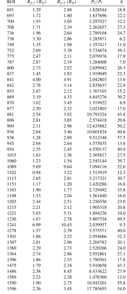
We list the key observed properties of Kepler two-planet
systems in Table 1, three-planet systems in Table 2,
four-planet systems in Table 3, and those systems with more than
four planets in Table 4. Planet indices given in these tables
signify orbit order, with one being the planet with the shortest period. These do not always correspond to the post-decimal point portion (.01, .02, etc.) of the KOI number designation of these candidates given in B11, for which the numbers signify the order in which the candidates were identified. These tables are laid out differently from one another because of the difference in parameters that are important for systems with differing numbers of planets. In addition to directly observed properties, these tables contain results of the dynamical analyses discussed below.
We plot the period and radius of each activeKeplerplanetary
candidate observed during the first four and one-half months of spacecraft operations, with special emphasis on multi-planet
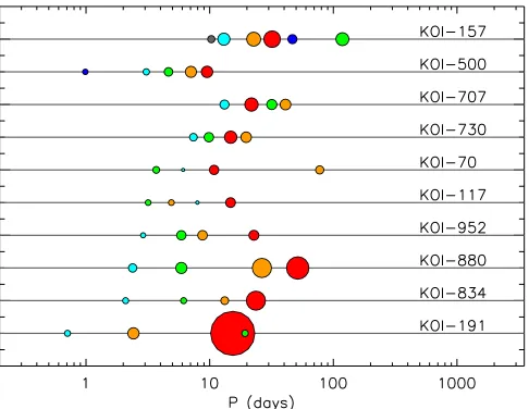
systems, in Figure 1. We present galleries of multi-planet
candidates, representing the planetary sizes and periods, in
Figures2–4. The ratio(s) of orbital periods is a key factor in
planetary system dynamics; the cumulative distributions of these period ratios for various classes of planetary pairings are plotted
in Figure5. Figure6 compares the cumulative distribution of
the period ratio of neighboring pairs ofKeplerplanet candidates
with the comparable distribution for radial velocity (RV) planets. The derivatives of these distributions with respect to period ratio, which show spikes near common period ratios, are displayed in Figure7.
The probability that aKeplertarget star hosts at least one
detected transiting planet is 961/160,171≈ 0.006, while the
probability that a star with one detected transiting planet hosts
at least one more is much higher, 170/961≈0.177. To
Table 1
Characteristics of Systems with Two Transiting Planets KOI Rp,1(R⊕) Rp,2(R⊕) P2/P1 Δ
72 1.30 2.29 54.083733 90.8
82 3.70 6.84 1.565732 7.6
89 4.36 5.46 1.269541 4.8
112 1.71 3.68 13.770977 55.7
115 3.37 2.20 1.316598 7.4
116 4.73 4.81 3.230779 21.6
123 2.26 2.50 3.274199 34.1
124 2.33 2.83 2.499341 25.5
139 1.18 5.66 67.267271 54.4
150 3.41 3.69 3.398061 26.3
153 3.07 3.17 1.877382 14.2
209 4.86 7.55 2.702205 14.8
220 2.62 0.67 1.703136 17.3
222 2.06 1.68 2.026806 20.5
223 2.75 2.40 12.906148 55.8
232 1.55 3.58 2.161937 20.1
244 2.65 4.53 2.038993 15.5
260 1.19 2.19 9.554264 70.3
270 0.90 1.03 2.676454 49.1
271 1.82 1.99 1.654454 17.5
279 2.09 4.90 1.846201 13.4
282 0.86 2.77 3.252652 36.0
291 1.05 1.45 3.876548 57.0
313 2.17 3.10 2.220841 21.0
314 1.95 1.57 1.675518 14.8
339 1.47 1.08 3.240242 50.6
341 2.26 3.32 1.525757 11.0
343 1.64 2.19 2.352438 28.6
386 3.40 2.90 2.462733 21.7
401 6.24 6.61 5.480100 23.3
416 2.95 2.82 4.847001 35.8
431 3.59 3.50 2.485534 19.6
433 5.78 13.40 81.440719 28.7
440 2.24 2.80 3.198296 30.0
442 1.43 1.86 7.815905 67.9
446 2.31 1.69 1.708833 15.5
448 2.33 3.79 4.301984 28.2
456 1.66 3.12 3.179075 31.6
459 1.28 3.69 2.810266 26.6
464 2.66 7.08 10.908382 33.2
474 2.34 2.32 2.648401 28.7
475 2.36 2.63 1.871903 17.0
490 2.29 2.25 1.685884 15.1
497 1.72 2.49 2.981091 33.8
508 3.76 3.52 2.101382 16.3
509 2.67 2.86 2.750973 25.6
510 2.67 2.67 2.172874 20.6
518 2.37 1.91 3.146856 32.3
523 2.72 7.31 1.340780 4.9
534 1.38 2.05 2.339334 28.7
543 1.53 1.89 1.371064 11.1
551 1.79 2.12 2.045843 23.5
555 1.51 2.27 23.366026 77.3
564 2.35 4.99 6.073030 34.0
573 2.10 3.15 2.908328 28.3
584 1.58 1.51 2.138058 28.5
590 2.10 2.22 4.451198 44.3
597 1.40 2.60 8.272799 59.7
612 3.51 3.62 2.286744 18.1
638 4.76 4.15 2.838628 19.5
645 2.64 2.48 2.796998 28.9
657 1.59 1.90 4.001270 42.5
658 1.53 2.22 1.698143 18.1
663 1.88 1.75 7.369380 52.0
672 3.98 4.48 2.595003 18.8
676 2.94 4.48 3.249810 20.4
Table 1
(Continued)
KOI Rp,1(R⊕) Rp,2(R⊕) P2/P1 Δ
691 1.29 2.88 1.828544 18.8
693 1.72 1.80 1.837696 22.2
700 1.93 3.05 3.297027 32.2
708 1.71 2.19 2.262657 27.3
736 1.96 2.64 2.789104 24.7
738 3.30 2.86 1.285871 6.2
749 1.35 1.98 1.357411 11.0
752 2.69 3.39 5.734874 39.3
775 2.47 2.11 2.079976 17.9
787 2.87 2.19 1.284008 7.0
800 2.73 2.52 2.659942 26.3
837 1.45 1.83 1.919049 22.3
841 4.00 4.91 2.042803 13.0
842 2.78 3.14 2.835637 22.9
853 2.87 2.12 1.767103 15.2
869 3.19 4.33 4.845276 30.2
870 3.62 3.45 1.519922 8.9
877 2.50 2.32 2.021803 17.0
881 2.54 3.92 10.793324 43.8
896 2.81 3.85 2.574418 20.6
904 2.11 2.96 12.635882 50.2
936 2.04 3.46 10.601824 40.6
938 1.28 2.89 9.512348 57.5
945 2.04 2.64 1.575035 13.6
954 2.35 2.45 4.550137 40.9
1015 1.63 2.36 2.305817 27.5
1060 1.23 1.54 2.545144 39.7
1089 5.69 9.64 7.094116 22.6
1102 0.94 3.22 1.513919 12.3
1113 2.65 2.81 3.217321 30.7
1151 1.17 1.20 1.420286 16.6
1163 1.90 1.77 2.729492 33.8
1198 1.53 2.04 1.561840 16.0
1203 2.44 2.51 2.256556 23.0
1215 2.21 2.12 1.905318 20.8
1221 5.03 5.31 1.694236 10.0
1236 1.67 2.78 5.807534 49.5
1241 6.99 10.43 2.039957 9.3
1278 1.57 2.39 3.575571 40.0
1301 1.86 2.32 2.954666 32.3
1307 2.81 2.96 2.204782 20.1
1360 2.29 2.73 2.520266 24.0
1364 2.74 2.86 2.952861 27.1
1396 1.86 2.53 1.790301 17.8
1475 1.79 2.18 5.910858 43.3
1486 2.38 8.45 8.433622 27.9
1589 2.23 2.28 1.476360 12.0
1590 1.90 2.75 10.943201 55.8
1596 2.26 3.45 17.785655 54.0
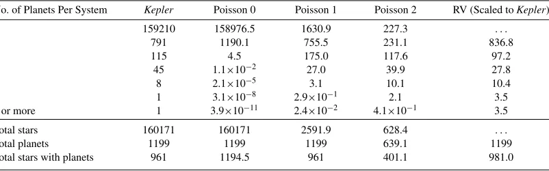
In the first of these synthetic populations, each of 1199 planets is randomly assigned to one of 160,171 stars. The number of stars
containingjplanets in this random population is equivalent to a
Poisson distribution with a mean of 1199/160,171≈0.0075 and
is denoted as “Poisson 0.” For the second synthetic population, “Poisson 1,” we again use a Poisson distribution, also forced to
match the observed total number ofKeplerplanets, 1199, but in
this case the second requirement is to match the total number of planetary systems (stars with at least one observed planet), 961, rather than the total number of stars, 160,171. Results are shown
in Table5, which also includes comparisons to a third random
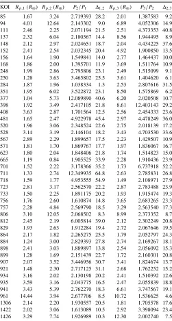
Table 2
Characteristics of Systems with Three Transiting Planets
KOI Rp,1(R⊕) Rp,2(R⊕) P2/P1 Δ1,2 Rp,3(R⊕) P3/P2 Δ2,3
85 1.67 3.24 2.719393 28.2 2.01 1.387583 9.2
94 4.01 12.64 2.143302 9.0 6.89 4.052306 14.9
111 2.46 2.25 2.071194 21.5 2.51 4.373353 40.8
137 2.32 6.04 2.180367 14.4 8.56 1.944495 8.9
148 2.12 2.97 2.024651 18.7 2.04 4.434225 37.6
152 2.41 2.54 2.032345 20.4 4.92 1.900850 13.5
156 1.64 1.90 1.549841 14.0 2.77 1.464437 10.0
168 1.86 2.00 1.395701 11.9 3.69 1.511764 10.9
248 1.99 2.86 2.795806 23.1 2.49 1.515099 9.1
250 1.28 3.63 3.465802 25.5 3.61 1.404620 6.1
284 1.87 1.96 1.038334 1.3 2.53 2.807616 31.5
351 1.95 6.02 3.522872 23.1 8.50 1.575869 6.2
377 1.04 5.73 12.089890 40.6 6.20 2.020508 10.7
398 1.92 3.49 2.417105 21.8 8.61 12.403143 29.2
408 3.63 2.87 1.701564 12.5 2.56 2.454333 23.6
481 1.65 2.47 4.922978 45.4 2.97 4.478249 36.0
520 1.96 3.06 2.348524 22.6 2.75 2.018139 17.2
528 3.14 3.19 2.146104 18.2 3.43 4.703530 33.6
567 2.89 2.29 1.899657 17.5 2.23 1.429507 10.9
571 1.81 1.70 1.869767 17.7 1.97 1.836067 16.7
623 1.80 2.04 1.848406 21.8 1.74 1.514823 15.0
665 1.19 0.84 1.905525 33.9 2.28 1.910436 23.9
701 1.52 2.22 3.178366 35.2 1.73 6.737918 52.2
711 1.33 2.74 12.349935 64.8 2.63 2.785831 26.8
718 1.59 1.77 4.953555 54.9 1.49 2.108971 27.9
723 2.81 3.17 2.562570 22.2 2.87 2.783488 23.9
733 1.50 2.25 1.891175 20.2 1.93 1.915474 19.3
756 1.76 2.60 1.610874 14.8 3.65 2.683265 23.3
757 2.28 4.84 2.569790 18.5 3.29 2.563540 17.3
806 3.10 12.05 2.068502 8.3 8.99 2.373352 8.7
812 2.45 2.19 6.005814 39.0 2.12 2.302249 20.8
829 1.93 2.63 1.912284 19.4 2.72 2.067646 19.5
864 2.17 1.82 2.265275 25.5 1.79 2.052797 24.3
884 1.24 3.00 2.829393 27.8 2.74 2.169267 18.1
898 2.41 3.03 1.889897 13.8 2.54 2.056092 15.3
899 1.28 1.69 2.151439 22.7 1.72 2.160301 20.8
907 2.07 3.52 3.446956 30.7 3.41 1.824674 13.7
921 1.48 2.30 2.717125 31.1 2.68 1.762252 15.2
934 3.16 2.02 2.130198 20.2 2.41 1.510392 12.6
935 3.59 3.16 2.043775 16.5 2.47 2.055839 18.8
941 3.43 5.39 2.762270 18.3 6.61 3.747567 19.1
961 14.44 3.94 2.677706 8.5 10.72 1.536625 4.6
1306 2.14 2.20 1.930557 20.5 1.81 1.705578 17.6
1422 2.02 3.06 1.613089 10.5 2.92 3.398094 23.4
1426 3.29 7.74 1.926989 10.3 12.30 2.002740 7.5
of planets as theKeplercandidates considered here. There are
sharp differences betweenKeplerobservations and Poisson 0:
the number of observedKeplermulti-transiting systems greatly
exceeds the random distribution, showing that transiting planets
tend to come in planetary systems, i.e., once a planet is detected to transit a given star, that star is much more likely to be orbited by an additional transiting planet than would be the case if transiting planets were randomly distributed among targets. Poisson 1, the random distribution that fits the total number of planets and the total number of stars with planets, underpredicts the numbers of systems with three or more planets, suggesting that there is more than one population of planetary systems. To carry the study further, we used a third random distribution, “Poisson 2,” constrained to fit the observed numbers of multi-planet systems (170) and multi-planets within said systems (408). The
Poisson 2 random distribution fits the numbers ofKeplersystems
with multiple transiting planets quite well, but it only accounts
for ∼35% of the single planet systems detected. As Kepler
does not detect all planets orbiting target stars for which some planets are observed, the observed multiplicities differ from the
true multiplicity; we explore these differences in Section6.
It is difficult to estimate the corresponding distribution for planets detected through Doppler RV surveys, since we do not know how many stars were spectroscopically surveyed for planets for which none were found. However, a search through
the Exoplanet Orbit Database (Wright et al.2011) as of 2011
January shows that 17% of the planetary systems detected by RV surveys are multi-planet systems (have at least two planets),
compared to 18% for Kepler. Including a linear RV trend as
evidence for an additional planetary companion, Wright et al.
(2009) show that at least 28% of known RV planetary systems
are multiple. Note, however, that the radial velocity surveys are generally probing a population of more massive planets
and one that includes longer period planets than the Kepler
sample discussed here. Some of the most recent RV planets are from the same population of small-planet, short-period multiples
seen in theKeplerdata (e.g., Lo Curto et al.2010; Lovis et al.
2011). Also, the observed multiplicity of RV systems is far less
sensitive to the mutual inclinations of planetary orbits than is the
multiplicity ofKeplercandidates. The final column in Table5
shows the distribution of RV detected planets normalized to the
total number ofKeplercandidates.
In systems with multiple transiting candidates, the ratio(s) of planetary periods and the ratio(s) of planetary radii are well measured independently of uncertainties in stellar properties. This suggests an investigation into whether outer planets are larger than inner planets on average, in order to provide constraints on theories of planet formation. (The ratio of orbital
periods is discussed in Section5.) When considering the entire
multi-candidate population, there is a slight but significant
preference for outer planets to be larger (Figure 1). However,
since planets with longer periods transit less frequently, all
else being equal the S/N scales asP−2/3, after accounting for
[image:4.612.57.559.648.750.2]the increase in S/N due to longer duration transits (assuming
Table 3
Characteristics of Systems with Four Transiting Planets
KOI Rp,1(R⊕) Rp,2(R⊕) P2/P1 Δ1,2 Rp,3(R⊕) P3/P2 Δ2,3 Rp,4(R⊕) P4/P3 Δ3,4
70 1.60 0.60 1.649977 22.6 2.27 1.779783 20.8 1.97 7.150242 53.5
117 1.29 1.32 1.541373 19.4 0.68 1.623476 25.1 2.39 1.853594 22.3
191 1.39 2.81 3.412824 35.8 11.56 6.350795 20.2 1.49 1.258207 2.9
707 2.19 3.36 1.652824 13.4 2.48 1.459577 9.8 2.64 1.290927 7.3
730 1.83 2.29 1.333812 9.4 3.09 1.500997 11.0 2.63 1.333948 7.5
834 1.39 1.39 2.943873 44.2 1.85 2.149832 28.5 4.87 1.787503 12.5
880 2.01 2.76 2.476866 25.6 4.90 4.480164 28.7 5.76 1.948715 11.1
Figure 1.Planet period vs. radius for all 1199 planetary candidates from B11 that we consider herein. Those planets that are the only candidate for their given star are represented by black dots, those in two-planet systems as blue circles (open for the inner planets, filled for the outer ones), those in three-planet systems as red triangles (open for the inner planets, filled for the middle ones, filled with black borders for the outer ones), those in four planet systems as purple squares (inner and outer members filled with black borders, second members open, third filled), the five candidates of KOI-500 as orange pentagons and the six planets orbiting KOI-157 (Kepler-11) as green hexagons. It is immediately apparent that there is a paucity of giant planets in multi-planet systems; this difference in the size distributions is quantified and discussed by Latham et al. (2011). The upward slope in the lower envelope of these points is caused by the low S/N of small transiting planets with long orbital periods (for which few transits have thus far been observed). Figure provided by Samuel Quinn.
Table 4
Characteristics of Systems with Five or Six Transiting Planets
Property KOI-500 KOI-157 (Nominal Kepler-11) Kepler-11 (Lissauer et al.2011)
Rp,1(R⊕) 1.23 1.70 1.97±0.19
Rp,2(R⊕) 1.47 3.03 3.15±0.30
P2/P1 3.113327 1.264079 1.26410
Δ12 40.5 6.8 7.0
Rp,3(R⊕) 2.06 3.50 3.43±0.32
P3/P2 1.512077 1.741808 1.74182
Δ23 12.7 13.1 15.9
Rp,4(R⊕) 2.75 4.21 4.52±0.43
P4/P3 1.518394 1.410300 1.41031
Δ34 10.4 7.3 10.9
Rp,5(R⊕) 2.83 2.22 2.61±0.25
P5/P4 1.349929 1.459232 1.45921
Δ45 6.8 8.8 13.3
Rp,6(R⊕) . . . 3.24 3.66±0.35
P6/P5 . . . 2.535456 2.53547
Δ56 . . . 24.1 . . .
Table 5
Comparison of Observed Distributions of Planetary System Multiplicity with Random Distributions
No. of Planets Per System Kepler Poisson 0 Poisson 1 Poisson 2 RV (Scaled toKepler)
0 159210 158976.5 1630.9 227.3 . . .
1 791 1190.1 755.5 231.1 836.8
2 115 4.5 175.0 117.6 97.2
3 45 1.1×10⁻² 27.0 39.9 27.8
4 8 2.1×10⁻⁵ 3.1 10.1 10.4
5 1 3.1×10⁻⁸ 2.9×10⁻¹ 2.1 3.5
6 or more 1 3.9×10⁻¹¹ 2.4×10⁻² 4.1×10⁻¹ 3.5
Total stars 160171 160171 2591.9 628.4 . . .
Total planets 1199 1199 1199 639.1 1199
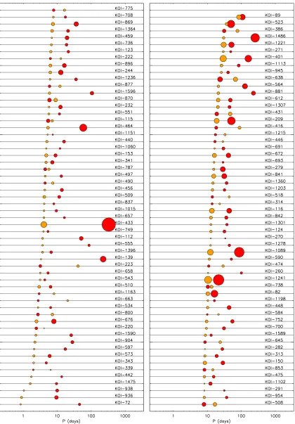
[image:5.612.108.509.596.721.2]Figure 2.Gallery of candidate planetary systems of 4–6 planets. Each horizontal line represents a separate system, as labeled. They are sorted by, first, the number of candidates, and second, the innermost planet’s orbital period. The size of each dot is proportional to the size of the planet that it represents, and in each system the size orderings move from hot (large) to cool (small) colors (red for the largest planet within its system, then gold, green, aqua, and, if additional planets are present, navy and gray). There is a clear trend for smaller planets to be interior to larger planets, but this is due to the greater detectability of small planets at shorter orbital period (Figure8).
(A color version of this figure is available in the online journal.)
circular orbits). To debias the radius ratio distribution, each planetary system is investigated and if the smallest planet
cannot be detected at S/N>16 if it were placed in the longest
period, that planet is removed. The remaining population of systems are not sensitive to observational bias, since each planet could be detected at all periods. The distribution of radius
ratios (Rp,o/Rp,i), where the subscripts o and i refer to the
inner and outer members of the pair of planets, for debiased
planetary systems is shown by the solid curve in Figure 8.
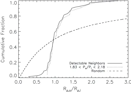
Interestingly, neighboring planets tend to have very similar radii,
with most of the population near Rp,o/Rp,i ≈ 1. This strong
tendency is illustrated by comparing the cumulative distribution of observed radii ratios with ratios of radii randomly drawn from
the debiased distribution (dashed curve in Figure8). Since there
is no requirement that the apparent depths of false positives and/
or planets to be comparable, this suggests that false positives are not common among systems with radii ratios near unity. In the debiased distribution, there is no significant preference for the outer planet to be larger than the inner one.
Examination of this debiased sample for additional non-trivial trends and correlations between radius ratio, period ratio, radius,
period, multiplicity, near-resonance (defined byζ1discussed in
Section5), and stellar properties, reveals a few additional clues
into the distribution of theKeplercandidates. When there is a
giant (R >6R⊕) planet, it is usually, but not always, at longer period. Radius ratios near 1 are almost exclusively found for
planets less than 4R⊕. Another trend is that whenever the period
ratio between two neighboring detectable planets exceeds 5, the sizes of the planets are similar and, conversely, large radius ratios
only occur for period ratios3. Furthermore, large period ratio
systems are only found around small stars (R < R). These
latter examples may be due to observational bias.
3. RELIABILITY OF THE SAMPLE
[image:6.612.319.568.54.599.2]Very few of the planetary candidates presented herein have been validated or confirmed as true exoplanets. As discussed in
Figure 3.Three planet candidate systems; same format as Figure2. (A color version of this figure is available in the online journal.)
B11, Brown (2003), and Morton & Johnson (2011), the
over-whelming majority of false positives are expected to come from eclipsing binary stars. Many of these will be eclipses of fainter
stars (physically associated with the target or background/faint
pro-Figure 4.Two planet candidate systems; same format as Figure2. (A color version of this figure is available in the online journal.)
grams that do not discriminate between single candidates and
systems of multiple planets. In addition, 1% of single and
multiple candidate systems were identified in subjective visual searches; this fraction is too small to significantly affect our statistical results.
The fact that planetary candidates are clustered around targets—there are far more targets with more than one candidate than would be expected for randomly distributed candidates
(Section2)—suggests that the reliability of the multi-candidate
[image:7.612.97.517.53.656.2]1 1.5 2 2.5 3 3.5 4 4.5 5 0
50 100 150 200 250 300
Period Ratio
N
[image:8.612.322.567.54.257.2]All adjacent pairings All pairings All 2−candidate pairings All adjacent 3−candidate pairings All 3−candidate pairings Inner 3−candidate pairings Outer 3−candidate pairings All adjacent 4−5−6−candidate pairings All 4−5−6 candidate pairings
Figure 5.Cumulative number,N, of pairs ofKeplerplanets orbiting the same star with period ratio,P(≡Po/Pi), less than the value specified. Black dashed curve
shows all pairings, solid black curve shows pairings of neighboring planets; solid red curve shows all pairings in two candidate systems; dashed blue curve shows all pairings in three-planet systems, solid blue curve shows all adjacent pairings in three-planet systems, solid light green curve shows inner pair of planets in three-planet systems, the solid dark green curve shows outer pair of planets in three-planet systems, the dashed pink curve shows all pairings in the 4, 5, and 6 planet systems, solid pink curve shows neighboring pairings in the 4, 5, and 6 planet systems. Sixty-five pairs of planets in the same system, including 31 adjacent pairs, haveP>5 and are not represented on this plot.
We know from RV observations that planets frequently come
in multiple systems (Wright et al.2009), whereas astrophysical
false positives are expected to be nearly random. The mere presence of multiple candidates increases our confidence that most or all are real planets, since the probability of multiple false positive signals is the product of the probabilities of two or more
relatively rare cases (Ragozzine & Holman2010). (Triple star
systems would be dynamically unstable for most of the orbital period ratios observed. Their dynamics would also give rise
to very large eclipse timing variations (e.g., Carter et al.2011),
which are generally not seen.) Additionally, the concentration of candidate pairings with period ratio near first-order MMRs such
as 3:2 and 2:1 (Figures5and7) suggests that these subsamples
likely have an even larger fraction of true planets, since such concentrations would not be seen for random eclipsing binaries. These qualitative factors have not yet been quantified.
Strong TTV signals are no more common for planets in observed multi-transiting candidates than for single candidates
(Ford et al.2011), and it is known that some of these systems
are actually stellar triples masquerading as planetary systems, suggesting that large TTVs are often the result of stellar systems
masquerading as planetary systems (e.g., Steffen et al.2011).
Nonetheless, it is possible that weaker TTVs correlate with multi-transiting systems, but that these small TTVs (e.g., those
in the Kepler-11 planetary system; Lissauer et al.2011) require
more data and very careful study to reveal.
The ratio of transit durations normalized to the observed periods of candidates in multi-transiting systems can also be used to identify false positives (generated by a blend of two objects eclipsing two stars of different densities) or as a probe of the eccentricity and inclination distributions. Transit durations depend upon orbital period, and it is convenient to normalize values for candidates in a system by dividing
measured duration byP1/3; this normalization would yield the
1 1.5 2 2.5 3 3.5 4 4.5 5
0 1
N
/
N TOT < 5
Period Ratio
1 1.5 2 2.5 3 3.5 4 4.5 5
Kepler adjacent pairings RV adjacent pairings
1 10 100
0 0.2 0.4 0.6 0.8 1
N
/
N TOT
Period Ratio
[image:8.612.47.295.57.260.2]Kepler adjacent pairings RV adjacent pairings
Figure 6.Cumulative fraction of neighboring planet pairs forKeplercandidate multi-planet systems with period ratio less than the value specified (solid curve). The cumulative fraction for neighboring pairs in multi-planet systems detected via radial velocity is also shown (dashed curve) and includes data from exoplanets.org as of 2011 January 29. (a) Linear horizontal axis, same as in Figure5. The data are normalized for the number of adjacent pairs with P<5, which equals 207 for theKeplercandidates and 28 for RV planets. (b) Logarithmic horizontal axis. All 238Keplerpairs are shown; the three RV pairs withP >200 are omitted from the plot, but used for the calculation ofNtot, which is equal to 61.
1 1.5 2 2.5 3 3.5 4 4.5 5
0 20 40 60 80 100 120 140 160 180 200
Period Ratio
Slope of Cumulative Period Ratio
Kepler adjacent pairings RV adjacent pairings
Figure 7.Slope of the cumulative fraction ofKeplerneighboring planet pairs (solid black curve) and multi-planet systems detected via radial velocity (dashed red curve) with period ratio less than the value specified. The slope for theKepler
curve was computed by taking the difference in period ratio between points with
Ndiffering by 4 and dividing this difference by 4. The slope for the RV curve was computed by taking the difference in period ratio between points withN
differing by 3 and dividing by 3, and then normalizing by multiplying the value by the ratio of the number ofKeplerpairings to the number of radial velocity pairings (3.9). The spikes in both curves nearP=2 and theKeplercurve near P=1.5 show excess planets piling up near period commensurabilities. Two points on theKeplercurve near period ratio 1.5 lie above the plot, with the highest value being 299.84; this sharp peak is produced by the excess of observed planet pairs in or very near the 3:2 mean motion resonance.
same value for planets of differing periods on circular orbits with the same impact parameter around the same star. For this study, we assumed circular orbits and a random distribution
[image:8.612.321.566.364.569.2]Figure 8.Cumulative distribution of the ratio of planetary radii (Rp,o/Rp,i)
for neighboring pairs of transiting planet candidates for which both planets are detectable at the longer period. The distribution of radii ratios for all such neighboring pairs (solid line, 71 ratios) is the same (within statistical uncertainty) as that of such pairs of planet candidates that are near the 2:1 mean motion resonance (dotted line, 22 ratios). Interestingly, neighboring planets tend to have very similar radii, with most of the population nearRp,o/Rp,i ≈1. This strong tendency is illustrated by showing for contrast the cumulative distribution of ratios between radii randomly drawn from the debiased distribution (dashed line). In the debiased distribution, there is no significant preference forRp,oto be greater or less thanRp,i.
that the distribution of normalized transit duration ratios is consistent with that of a population of planetary systems with no contamination. The consistency of normalized duration ratios is not a strong constraint for false positives, but the observed systems also pass this test.
There are five pairs for which the observed transit duration ratio falls in the upper or lower 5% of the distribution predicted. These are KOI-864.01 and 864.03, 291.02 and 291.01, 1426.01 and 1426.03, 645.01 and 645.02, and 1089.02 and 1089.01; in-dependent evidence from the shape of the transit light curve
indicates that KOI-1426.03’s transits are grazing (Section4).
However, this test is not definitive enough to rule out the plan-etary interpretation, in favor of a blended eclipsing binary hy-pothesis, for any of these pairs. Given 238 pairs of neighboring planets among the multiple planet candidate systems identified by Kepler, a 10% false alarm rate (corresponding to the ex-treme 5% on either side of the distribution) could easily result in nearly two dozen such pairs of planets simply due to chance. The substantially smaller fraction of extreme normalized
du-ration ratios that are observed may result from the lower S/N
(and thus decreased likelihood for detection) of grazing and
near-grazing transits. In sum, wedo notfind evidence for false
positives based on the ratio of transit durations of KOIs with a common host star.
4. LONG-TERM STABILITY OF PLANETARY SYSTEMS
Keplermeasures planetary sizes, whereas masses are the key parameters for dynamical studies. For our dynamical studies, we
convert planetary radii,Rp, to masses,Mp, using the following
simple formula:
Mp= R
p
R⊕ 2.06
M⊕, (1)
where R⊕ andM⊕ are the radius and mass of the Earth,
respectively. The power law of Equation (1) was obtained by
fitting to Earth and Saturn; it slightly overestimates the mass of
Uranus (17.2M⊕ versus 14.5M⊕) and slightly underestimates
the mass of Neptune (16.2M⊕ versus 17.1M⊕). (Note that
Uranus is larger, but Neptune is more massive, so fitting both with a monotonic mass–radius relation is not possible.)
Observations of transiting exoplanets (Lissauer et al.2011, and
references therein) show more significant deviations from the
relationship given by Equation (1) than do Uranus and Neptune,
with both denser and less dense planets known, but on average the known exoplanets smaller than Saturn are consistent with this general trend. The stellar mass, taken from B11, was derived
from theRand loggestimates from color photometry of the
KIC (Brown et al.2011).
A convenient metric for the dynamical proximity of thejth
and (j+ 1)th planets is the separation of their orbital semi-major
axes,aj+1−aj, measured in units of their mutual Hill sphere
radius (Hill1878; Smith & Lissauer2010):
RHj,j+1=
Mj +Mj +1
3M
1/3(aj +aj+1)
2 , (2)
where the index j = (1, Np −1), withNp being the number
of planets in the system under consideration,Mjandajare the
planetary masses and semi-major axes, andM is the central
star’s mass (the masses of interior planets are likely to be much smaller than the uncertainty in the star’s mass, and thus have
been neglected in Equation (2)).
The dynamics of two-planet systems are a special case of the three-body problem that is amenable to analytic treatment and simple numerically derived scaling formulae. For instance, a pair of planets initially on coplanar circular orbits with dynamical orbital separation
Δ≡ ao−ai
RH
>2√3≈3.46 (3)
can never develop crossing orbits and are thus called “Hill
stable” (Gladman1993). Dynamical orbital separations of all
planet pairs in two-planet systems for stellar masses given in
B11 and planetary masses given by Equation (1) are listed in
Table1. We see that all two-planet systems obey the criterion
given in Expression (3). This is additional evidence in favor
of a low false positive rate, as random false positives would occasionally break this criterion.
The actual dynamical stability of planetary systems also de-pends on the eccentricities and mutual inclination (Veras &
Armitage2004), none of which can be measured well from the
transit data alone (cf. Ford et al.2011). Circular coplanar orbits
have the lowest angular momentum deficit (AMD), and thus
are the most stable (Laplace 1784; Laskar 1997). An
excep-tion exists for planet pairs protected by MMRs (Secexcep-tion 5.4)
that produce libration of the relative longitudes of various com-binations of orbital elements and prevent close approaches. A second exception exists for retrograde orbits (Smith & Lissauer
2009), but these are implausible on cosmogonic grounds
(Lissauer & Slartibartfast2008). Hence, theKeplerdata can only
be used to suggest that a pair of planets is not stable. Instability is particularly likely if their semi-major axes are closer than the
resonance overlap limit (Wisdom1980; Malhotra1998):
2ao−ai
ai+ao
<1.5
Mp M
2/7
. (4)
Equation (4) was derived only for one massive planet; the other
masses, eccentricities, and mutual inclinations can be inferred from the requirement that the planetary systems are presumably stable for the age of the system, which is generally of order
1011times longer than the orbital timescale for the short-period
planets that represent the bulk ofKepler’s candidates. However,
we may turn the observational problem around: the ensemble of duration measurements can be used to address the eccentricity
distribution (Ford et al.2008); since multi-planet systems have
eccentricities constrained by stability requirements, they can be
used as a check to those results (Moorhead et al.2011).
Systems with more than two planets have additional dynam-ical complexity, but are very unlikely to be stable unless each
neighboring pair of planets satisfies Expression (3). Nominal
dynamical separations (Δ’s) between neighboring planet pairs
in three-planet systems are listed in Table2, the separations in
four-planet systems are listed in Table3, and those for the
five-planet and six-five-planet systems in Table4. We find that in the
overwhelming majority of these cases, the inequality in Expres-sion (3) is satisfied by quite a wide factor.
Smith & Lissauer (2009) conducted suites of numerical
integrations to examine the stability of systems consisting of
equal mass planets that were equally spaced in terms of Δ.
They demonstrated dynamical survival of systems with three
comparably spaced 1M⊕planets orbiting a 1Mstar for 1010
orbits of the inner planet in cases where the relative spacing between orbital semi-major axes exceeded a critical number
(Δcrit ∼ 7) of mutual Hill spheres. For systems with five
comparably spaced 1M⊕ planets, they foundΔcrit ≈ 9. Their
calculations give slightly largerΔcritfor systems of five 0.33M⊕
planets, suggesting a slightly smaller Δcrit for the somewhat
larger planets that dominate theKeplersample of interest here.
Systems with planets of substantially differing masses tend to be less stable because a smaller fraction of the AMD needs to be placed in the lowest mass planets for orbits to cross. Taking all of these factors, as well as the likely presence of undetected planets
in many of the systems, into account, we considerΔcrit ≈9 to
be a rough estimate of how close planetary orbits can be to have a reasonable likelihood of survival on Gyr timescales.
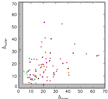
For each adjacent set of three planets in our sample, we plot
theΔseparations of both the inner and the outer pairs in Figure9.
We find that in some casesΔ <9, but the other separation is
quite a bit larger thanΔcrit. In our simulations of a population of
systems in Section6, we impose the stability boundary:
Δi+Δo>18, (5)
which accounts for this possibility, in addition to requiring
that inequality in Expression (3) is satisfied. The form of
Expression (5) is motivated by observations within our solar
system (Lissauer1995).
We investigated long-term stability of all 55 systems with three or more planets using the hybrid integrator within the
Mercurypackage (Chambers1999). We set the switchover at
3 Hill radii, but in practice we aborted simulations that violated
this limit, so for the bulk of the simulation then-body mapping
of Wisdom & Holman (1991) was used, with a time step of 0.05
times as large as the orbital period of the innermost planet. The
simplest implementation (Nobili & Roxburgh1986) of general
relativistic precession was used, an additional potential
UGR= −3
GM cr
2
, (6)
where Gis Newton’s constant, c is the speed of light, andr
[image:10.612.331.553.53.257.2]is the instantaneous distance from the star. More sophisticated
Figure 9.Orbital separations, expressed in mutual Hill radii (Equation (2)), for the inner (Δi) and outer (Δo) pairs within planet systems and adjacent three-planet sub-systems of the four-, five-, and six-three-planet systems of our sample. The colored symbols are the same as in Figure1, and we also include the spacings of planets within the solar system as black circles. Gray region: stability boundary for two-planet systems,Δ > 2√3 (Expression (3)). Dashed line: stability boundary used for the simulated population of multi-planet systems: Δi+Δo >18; some of the nominal systems survived long-term integrations despite transgressing that boundary. The unstable nominal systems KOI-191 and KOI-248 both lie within the gray region, and all the long-term survivors are outside of it.
(A color version of this figure is available in the online journal.)
treatments of general relativity (Saha & Tremaine 1994) are
not yet required, due to the uncertainties of the masses of the planets and stars whose dynamics are being modeled. We neglected precession due to tides on or rotational flattening in the planets, which are only significant compared to general relativity for Jupiter-size planets in few-day orbits (Ragozzine
& Wolf2009), and precession due to the rotational oblateness
of the star, which can be significant for very close-in planets of any mass. Precession due to the time-variable flattening of the star can generate a secular resonance, compromising stability
(Nagasawa & Lin 2005); we neglected this effect, treating
the star as a point mass. We also neglect tidal damping of eccentricities, which can act to stabilize systems over long timescales, and tidal evolution of semi-major axes, which sometimes has a destabilizing effect. We assumed initially circular and coplanar orbits that matched the observed periods
and phases, and chose the nominal masses of Equation (1).
For the triples, quadruples, and the five-planet system
KOI-500, we ran these integrations for 1010 orbital periods of
the innermost planet and found the nominal system to be stable for this span in nearly all cases; the two exceptions are described below. The most populous transiting planetary system discov-ered so far is the six-planet system Kepler-11. In the discovery
paper, Lissauer et al. (2011) reported a circular model, with
physically plausible. Introducing a small amount of eccentricity can compromise stability, but our results do not exclude ec-centricities of a few percent because (1) planetary masses have significant uncertainties, and we have not conducted a survey
of allowed mass/eccentricity combinations, and (2) tidal
damp-ing of eccentricities may be a significant stabilizdamp-ing mechanism over these timescales for planets orbiting as close to their star as are Kepler-11b and c. Future work should address the limits imposed on the eccentricities by the requirement that the system remains stable for several Gyr.
Only two systems became unstable at the nominal masses:
KOI-284 and KOI-191; KOI-191 is discussed in Section5.4.
KOI-284 has a pair of candidates with periods near 6 days and
a period ratio 1.0383 and an additional planet at 18 days. Both
of the 6 day planets would need to have masses about that of
the Earth or smaller for the system to satisfy Expression (3)
and thus be Hill stable. But the vetting flags are 3 for both of these candidates—meaning that they are suspect candidates for
other reasons—and theKeplerdata display significant correlated
noise that may be responsible for these detections. We expect one or both of these candidates are not planets, or if they are, they are not orbiting the same star. This is the only clear example of
a dynamically identified likely false positive in the entireKepler
multi-candidate population.
In our investigation, we also were able to correct a poorly fit
radius of 35R⊕(accompanied by a grazing impact parameter in
the original model, trying to account for a “V” shape) for KOI-1426.03, which resulted in too large a nominal mass, driving the system unstable. It is remarkable that stability considerations allowed us to identify a poorly conditioned light curve fit. Once
the correction was made to 13R⊕, the nominal mass allowed
the system to be stable.
That so few of the systems failed basic stability measurements implies that there is not a requirement that a large number of planets have substantially smaller densities than given by the
simple formula of Equation (1). Stability constraints have the
potential to place upper limits on the masses and densities of candidates in multiply transiting systems, assuming that all the candidates are planets.
5. RESONANCES
The formation and evolution of planetary systems can lead to preferred occupation of resonant and near-resonant
config-urations (Goldreich 1965; Peale 1976; Malhotra 1998). The
abundance of resonant planetary systems provides constraints on models of planetary formation and on the magnitude of dif-ferential orbital migration.
The distribution of period ratios of multi-transiting candidates in the same system is significantly different from the distribu-tion obtained by taking ratios of randomly selected pairs of periods from all 408 multi-transiting candidates. Most observed planetary pairs are neither in nor very near low-order MMRs; nonetheless, the number of planetary pairs in or near MMRs
exceeds that of a random distribution (Figures5–7,10–12). In
this section, we quantify this clustering and discuss a few par-ticularly interesting candidate resonant systems.
5.1. Resonance Abundance Analysis
Kepler’s multi-planet systems provide a complementary data set to exoplanets detected in RV surveys, in that RV planets are typically larger and detected on the basis of mass rather than radius. RV multiples have the advantage of being minimally
1.0 1.5 2.0 2.5 3.0 3.5 4.0 1.0
0.5 0.0 0.5 1.0
Period Ratio
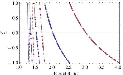
[image:11.612.339.551.55.184.2]ζ
Figure 10.Value ofζ as a function of period ratio for the first-order (solid, blue) and second-order (dashed, red) MMRs. Also shown are the observed period ratios in theKeplerdata.
(A color version of this figure is available in the online journal.)
biased by relative planetary inclinations. Multiply transiting planets have two advantages over RV planetary systems for the study of resonances: first, periods are measured to very high
accuracy, even for systems with moderately low S/N, so period
ratios can be confidently determined without the harmonic ambiguities that affect RV detections (Anglada-Escud´e et al.
2010; Dawson & Fabrycky 2010); however, transits can be
missed or noise can be mistaken for additional transits when the
S/N is very low. Second, resonances significantly enhance the
signal of TTVs (Agol et al.2005; Holman & Murray2005; Veras
& Ford2010), which can also be measured accurately, either to
demonstrate or confidently exclude resonance occupation, given
enough time (e.g., Holman et al.2010).
Planets can be librating in a resonance even when they have apparent periods that are not perfectly commensurate
(Peale 1976; Marcy et al. 2001; Rivera & Lissauer 2001;
Ragozzine & Holman 2010). Nevertheless, the period ratios
of resonant planets will generally be within a few percent of commensurability. In the cumulative distribution of period
ratios (Figure5), we see that few planets appear to be directly
in resonance (with the important exception of KOI-730), but placing limits on resonance occupation requires additional analysis.
In the solar system, there is a known excess of satellite pairs
near MMRs (Goldreich1965), and theoretical models of planet
formation and migration suggest that this may be the case for
exoplanets (e.g., Marcy et al. 2001; Terquem & Papaloizou
2007). Can such an excess be seen in the sample of multiply
transiting Keplerplanetary systems? To answer this question,
we divide the period ratios of the multiply transiting systems into “neighborhoods” that surround the first- and
second-order (j:j −1 and j:j −2) MMRs. The boundaries between
these neighborhoods are chosen at the intermediate, third-order MMRs. Thus, all candidate systems with period ratios less than 4:1 are in some neighborhood. For example, the neighborhood of the 3:1 MMR runs between period ratios of 5:2 and 4:1, for the 2:1 it runs from 7:4 to 5:2. With this algorithm, the first-order MMRs have neighborhoods (represented by solid lines
in Figure 10) that are essentially twice as large as those for
second-order MMRs (dashed lines in Figure10). The purpose of
dividing the period ratio distribution into neighborhoods around the major resonances is to account for the fact that even random period ratios can be close to some ratio of integers (Goldreich
1965).
We define a variable,ζ, that is a measure of the difference
neighbor-Table 6
Counts of Planet Pairs Found in Each Resonance Neighborhood
MMR Total Pairs Adjacent Pairs
2:1 89 78
3:2 22 22
4:3 7 7
5:4 3 3
3:1 79 55
5:3 15 15
7:5 5 5
9:7 3 3
hood. In order to treat all neighborhoods equally,ζ is scaled to
run from−1 to 1 in each neighborhood. For first-order MMRs,
ζ is given by
ζ1≡3
1
P−1 −Round
1
P−1
, (7)
whereP ≡Po/Piis the observed period ratio (always greater
than unity) and “Round” is the standard rounding function that returns the integer nearest to its argument. Similarly, for
second-order MMRs,ζ is given by
ζ2≡3
2
P−1 −Round
2
P−1
. (8)
Table6gives the number of planet pairs taken from Tables1–4
that are found in each neighborhood. The value ofζas a function
of the period ratio is shown together with the data in Figure10.
We also list neighborhood abundances considering only adjacent planet pairs. This last case primarily removes pairs in the neighborhood of the 3:1 MMR, but also a nontrivial fraction of those neighboring the 2:1 MMR. The fact that significant numbers of non-adjacent pairs are in these neighborhoods
demonstrates how closely packed many of the Kepler
multi-transiting systems are.
We calculate ζ for each planetary period ratio and stack
the results for all of the resonances in each MMR order. The
resulting distribution inζ is compared to a randomly generated
sample drawn from a uniform distribution in logP, a uniform
distribution inP, and from a sample constructed by taking the
ratios of a random set of the observed periods in the multiple candidate systems. This third sample has a distribution that is
very similar to the logarithmic distribution. Figure11 shows
a histogram of the number of systems as a function of ζ
for both the first-order and second-order MMRs. We see that the results for the second-order MMRs have some qualitative similarities to the first-order MMR, though the peaks and valleys are less prominent. In the tests described below, we also consider the case where all first- and second-order MMRs are stacked together, as well as this stacked combination with the likely
resonant systems KOIs 730, 191, and 500 (Sections5.3,5.4,
and5.5) removed in order to determine the robustness of our
results to the influence of a few special systems. Finally, we study the distribution of adjacent planets only.
To test whether the observed distributions inζ are consistent
with those from our various test samples, we took the absolute
value ofζ for each collection of neighborhoods and used the
Kolmogorov–Smirnov test (K-S test) to determine the probabil-ity that the observed sample is drawn from the same distribu-tion as our test sample. The results of these tests are shown in
Table7. Figure12shows that the probability density function
1.0 0.5 0.0 0.5 1.0 0.0
0.5 1.0 1.5 2.0
ζ
1.0 0.5 0.0 0.5 1.0 0.0
0.5 1.0 1.5 2.0
ζ
[image:12.612.334.552.51.341.2]Figure 11.Probability density of the systems as a function ofζ for first-order (top) and second-order (bottom) mean motion resonances. The most common values forζ for first-order resonances are small and negative, i.e., lie just outside the corresponding MMR, while one of the least common values, small and positive, lie just inside the MMR. No strong trends are observed for second-order resonances. The probability density for the logarithmically distributed test sample is a monotonically decreasing function and is shown for reference in both plots by white boxes for those values ofζfor which its value exceeds that of the data.
[image:12.612.67.271.77.182.2](A color version of this figure is available in the online journal.)
Table 7
K-S Testp-values for Different Resonance Sets and for Test Distributions
Resonance Set log(P) P AllKeplerMultis
2:1 only 0.00099 0.00011 0.00059
j:j−1 0.0012 0.00021 0.00044
j:j−2 0.046 0.0094 0.040
All (j:j−1 andj:j−2) 8.2×10⁻⁵ 2.7×10⁻⁷ 3.9×10⁻⁵ All except KOIs 191, 500, 730 0.0010 0.00014 0.00072 All adjacent pairs 9.7×10⁻⁶ 7.5×10⁻⁷ 7.5×10⁻⁶
(PDF) for the combined distribution of first- and second-order MMRs differs from the PDF for the logarithmically distributed sample.
A few notable results of these tests include (1) the distribu-tions observed within the combined first-order and second-order neighborhoods are distinctly inconsistent with any of the trial period distributions—including a restricted analysis where the likely resonant systems KOIs 191, 500, and 730 are excluded, (2) the distributions within the neighborhoods surrounding the first-order MMRs are also very unlikely to originate from the test distributions, (3) there is significant evidence that the dis-tributions within the neighborhood surrounding the 2:1 MMR alone are inconsistent with the test distributions, (4) there is a hint that the distributions in the neighborhoods of second-order resonances are not consistent with the test distributions,
[image:12.612.317.570.474.554.2]0.0 0.2 0.4 0.6 0.8 1.0 0.0
0.2 0.4 0.6 0.8 1.0
ζ
[image:13.612.59.279.57.196.2]CDF
Figure 12.Cumulative distribution function (CDF) of the absolute value ofζ for the combined first-order and second-order resonances (jagged distribution of large blue points). Also shown is the CDF for the logarithmically distributed test sample (red). The results of the K-S test for these two distributions are given in Table7along with the K-S test results for other combinations of resonances and test distributions.
(A color version of this figure is available in the online journal.)
data are necessary to produce higher significance results for the second-order resonances, and (5) when only adjacent planet pairs are considered, all of the test distributions are rejected with higher significance.
Given the distinct differences between our quasi-random test distributions and the observed distribution, a careful look at the
histograms shown in Figure11reveals that the most common
location for a pair of planets to reside is slightly exterior to the MMR (the planets are farther apart than the resonance location), regardless of whether the resonance is first order or second order. Also, a slight majority (just over 60%) of the period
ratios haveζ values between –1/2 and +1/2, while all of the
test distributions have roughly 50% between these two values in
ζ(note thatζ = ±1/2 corresponds to sixth-order resonances in
first-order neighborhoods and 12th-order resonances in second-order neighborhoods—none of which are likely to be strong for these planet pairs). There are very few examples of systems with planet pairs that lie slightly closer to each other than the first-order resonances, and for the second-order resonances only the 3:1 MMR has planet pairs just interior to it. Finally, there is a hint that the planets near the 2:1 MMR have a wider range of orbital periods, while those near the 3:2 appear to have shorter periods and smaller radii on average. While additional data are necessary to claim these statements with high confidence, the observations are nonetheless interesting and merit serious investigation to determine the mechanisms that might produce such distributions.
A preference for resonant period ratios cannot be exhibited by systems without direct dynamical interaction. Multiple star systems with similar orbital periods (i.e., non-hierarchical) are not dynamically stable, so dynamical interaction between
ob-jects with period ratios 5 indicates low masses, typically
in the planetary or brown dwarf regime. Thus, the prefer-ence for periods near resonances in our data set is statisti-cally significant evidence that most if not all of the candidate (near-)resonant systems are actually systems of two or more planets. Note, however, that assessing the probability of dy-namical proximity to resonance for the purpose of eliminating the false positive hypothesis in any particular system requires a specific investigation.
An excess of pairs of planets with separations slightly wider than nominal resonances was predicted by Terquem &
Papaloizou (2007), who pointed out that tidal interactions with
the star will, under some circumstances, break resonances. However, not all of the systems near resonance have short-period planets that would be strongly affected by tides. Interestingly, KOI-730 seems to have maintained stability and resonance occupation despite the short periods of the planets that imply susceptibility of the system to differential tidal evolution.
5.2. Frequency of Resonant Systems
RV planet searches suggest that roughly one-third of the multiple planet systems that have been well characterized by RV observations are near a low-order period commensurability,
with one-sixth near the 2:1 MMR (Wright et al.2011).Kepler
observations find that at least∼16% of multiple transiting planet
candidate systems contain at least one pair of transiting planets
close to a 2:1 period commensurability (1.83 < P < 2.18).
While it is tempting to consider these results as showing a similarity between the Jupiter-mass planets that dominate the RV sample and those of the Neptune-size planets that form the
bulk of theKeplercandidates, there are many differences in the
criteria used to identify these planets and to calculate the period ratios.
RV planets are spread over a much wider range of period ratio
than are theKepler candidates, and the concentration seen in
the RV planets is in the region very near the 2:1 MMR, whereas
the one-sixth number for theKeplercandidates is in the wider
“neighborhood” that we have defined. Wright et al.’s (2011)
estimate for RV systems near the 2:1 MMR may be lower than the actual value for the ensemble of systems that they considered because of detection biases. RV observations for systems near the 2:1 MMR have an approximate degeneracy with a single planet on an eccentric orbit. This degeneracy makes it difficult for RV observations to detect a low-mass planet in the interior
location of a 2:1 MMR (Giuppone et al.2009; Anglada-Escud´e
et al.2010).
Among RV-discovered systems, only one-quarter of the pairs near the 2:1 MMR have an inner planet significantly less massive
than the outer planet. The two exceptions (GJ 876 c&b,μAra
d&b) each benefited from a unusually large (100) numbers of
RV observations. Because of this degeneracy, it is possible that many 2:1 resonant systems with low-mass, interior members have been misidentified as eccentric single planets. Thus, the true rate of planetary systems near the 2:1 MMR may be significantly greater than one-sixth.
Also, the true fraction of Keplersystems near a 2:1 period
commensurability could be significantly greater than ∼16%,
since not all planets will transit. If we assume that planets near the 2:1 MMR are in the low inclination regime, then the outer
planet should transit abouta1/a2 ≈63% of the time, implying
that the true rate of detectable planets (in size–period space, not accounting for the geometrical limitations of transit photometry)
near the 2:1 MMR is25%. If a significant fraction of these
systems are not in the low inclination regime, then the true rate of pairs of planets near the 2:1 MMR would be even larger.
Based on the B11 catalog, neighboring transiting planet can-didates tend to have similar radii, and in the majority of cases, the outer planet is slightly larger. However, smaller planets are more easily detected in shorter-period orbits, and a debi-ased distribution shows no preference for the outer planet to
be larger (Section2). The distribution of planetary radii ratios
(Rp,o/Rp,i) for neighboring pairs of transiting planet candidates near a 2:1 period commensurability (MMR) is concentrated
be-tween 0.8 and 1.25 (see Figure8, dotted curve). For reasonable