Vibration analysis of a tyre model using the wave finite element method

19

th

INTERNATIONAL CONGRESS ON ACOUSTICS

MADRID, 2-7 SEPTEMBER 2007

VIBRATION ANALYSIS OF A TYRE MODEL USING THE WAVE FINITE

ELEMENT METHOD

PACS: 43.50.Lj

Waki, Yoshiyukia; Mace, Brianb; Brennan, Michaelc

ISVR, University of Southampton, Highfield, Southampton SO17 1BJ, United Kingdom; a

[email protected], [email protected], [email protected]

ABSTRACT

The vibration of a tyre is predicted using the wave finite element (WFE) method. The material properties are considered to be frequency dependent. The WFE method starts from a conventional finite element (FE) model of only a short section of a structure, which is uniform in one direction. Existing element libraries can be fully utilised and the size of the FE model can be very small. Free wave propagation characteristics are extracted from the dynamic stiffness matrix of the FE model. The forced response is calculated using the wave approach. An approach for determining the amplitudes of the directly excited wave is proposed to reduce numerical difficulties. The method is applied to a tyre FE model formed using ANSYS. The material properties of rubber are considered to be frequency dependent. The free wave propagation is shown including nearfield waves. The predicted forced response is compared with experimental data. Good agreement can be seen on the whole.

1. INTRODUCTION

Tyre noise is becoming a significant source of traffic noise [1] and understanding the vibrational behaviour of a tyre is thus becoming more important. At high frequencies, where FE models become impractically large, knowledge of the wave properties of a structure is of great value. Wave approaches can then be used. In this paper, the WFE method [2,3] is applied to model the free and forced vibration of a tyre. The formulation is first reviewed. Element matrices of a short section of a uniform structure are post-processed to yield the wave behaviour. The matrices can be obtained from a conventional FE method and a commercial package. This is in contrast to the spectral finite element method [4]. A short section of an unloaded tyre is modelled in ANSYS. Complete structural details can be included, which may be difficult in analytical approaches (e.g. [5]).

2. FORMULATION OF THE WFE METHOD

This section describes the formulation of the eigenvalue problem for determining free wave propagation characteristics from a conventional FE model.

2.1 Dynamic stiffness matrix

Consider a short section of length

∆

of a uniform waveguide. The dynamic equation of the section can be written as [3]

=

Dq

f

;

D

=

K

+

j

ω

C

−

ω

2

M

(Eq. 1)

where

D

is the dynamic stiffness matrix,

q

is the displacement vector,

f

is the force vector

and

K C M

, ,

are the stiffness, damping and mass matrices, which may be formed using a

LL LR L L

RL RR R R

=



    



    



    

D

D

q

f

D

D

q

f

(Eq. 2)

where the subscripts

L

and

R

represent the left and right hand side of the section.

2.2 Free wave propagation in a uniform waveguide

After applying the periodicity condition

q

_R

=

λ

q

_L, the transfer matrix can be expressed in the form of an eigenvalue problem as [2]

q q

f f

λ









=

















φ

φ

T

φ

φ

(Eq. 3)

where the transfer matrix

T

is formed from the elements of the dynamic stiffness matrix. The eigenvalues of (Eq. 3) represent the wavenumbers

k

, i.e.

jk_i

i

e

λ

− ∆

=

(Eq. 4)

for the ith wave mode. The wavenumbers may be real, imaginary or complex. The associated ith wave mode is given by the eigenvector;

T

T T

i

= 



qi fi





φ

φ

φ

(Eq. 5)

where

⋅

T is the transpose. The wave mode contains information about both the nodal displacements and associated internal forces. For uniform waveguides, there exist positive- and negative-going wave pairs of the form jki

i

e

λ

±

₌

∓ ∆

and the eigenvalues and associated

eigenvectors are

(

λ

_i

,

φ

_i+

)

and

(

1

λ

_i

,

φ

_i−

)

. The superscripts

±

represent positive- and

negative-going waves. Positive-negative-going waves are such that

λ

_i

<

1

or, if

λ

_i

=

1

, the energy flow is

positive, i.e.

Re

{ }

f q

H

>

0

where

⋅

H represents the complex conjugate transpose.

Numerical difficulties may occur when the eigenvalue problem, (Eq. 3), is formed and solved. Zhong’s method [6] may be used to improve the matrix conditioning. Numerical issues and implementations are discussed in detail in [7].

3. FORCED RESPONSE CALCULATION USING THE WAVE APPROACH

The forced response can be obtained using the wave approach. The amplitude of the directly excited waves is first found and the total wave amplitudes are determined by considering the propagation and reflection of the directly excited waves in general. A well-conditioned formulation to determine the amplitude of the excited waves is proposed.

3.1 Excited wave amplitude

When an external force is applied to an infinite waveguide, continuity of displacement and force equilibrium give

,

q q ext f f

+ +

₌

− −

₊

+ +

₋

− −

₌

Φ e

Φ e

f

Φ e

Φ e

0

(Eqs. 6)

where

e

± is a column vector of excited wave amplitudes,

f

_ext is the external force vector and the

matrices

Φ

_q±,

Φ

±_f contain the displacement or force eigenvectors, i.e.

Φ

_q±

=

_



φ

_q±₁

φ

±_qn

_



formed in the same manner as the right eigenvector matrix. The eigenvectors can be normalised so that

d

_i

=

1

and

Ψ Φ

T

=

I

, where

I

is the identity matrix. With the normalised eigenvectors, premultiplying (Eqs. 6) by

Ψ

T leads to

T T

,

.

q ext q ext

+

_{= −}

+ −

_{= −}

−

e

Ψ f

e

Ψ f

(Eqs. 7)

(Eqs. 7) are always well-conditioned. In practice, only the first

m

( )

≤

n

waves might be retained,

these being waves for which

Im

( )

k

are small. The rapidly decaying waves often give a small

contribution to the response.

3.2 Total wave amplitude

When a waveguide forms a ring or a toroidal shape such as a tyre, the wave amplitudes

a

± at the excitation point are given by

( )

{

}

1

{

( )

}

1

,

L

−

L

−

+

₌

₋

+ −

₌

₋

−

₋

−

a

I

τ

e

a

I

τ

e

e

(Eqs. 8)

where

τ

( )

L

is the wave propagation matrix whose diagonal elements are

_e

−jk Li _{, and}

_L

_{is the}

circumferential length of the waveguide. The displacement is then given by

(

)

1

n

i qi i qi

i

a

+ +

a

− −

=

=

∑

+

q

φ

φ

.

4. APPLICATION TO TYRE VIBRATION ANALYSIS

The WFE method is applied to a tyre model. The dispersion relationship is determined including nearfield waves. The point mobility is calculated and compared with experimental data.

4.1 Tyre model

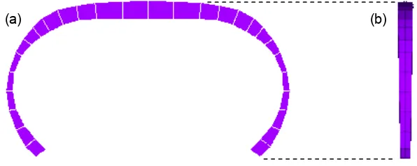
A test tyre with smooth tread (195/65R15) was provided by Bridgestone Corporation together with geometric and material property data. A section of the tyre was modelled using ANSYS 7.1 as shown in Figure 1. A tyre is a complicated structure which is composed of several different rubbers, steel and textile fibres. The solid element SOLID46, which generates equivalent single material properties for a layer structure, was used. A series of elements was concatenated to represent the curvature in the circumferential direction. The angle of 1.8 degrees in the circumferential direction was modelled. An internal pressure of 200kPa was simulated by the application of surface loads on the elements. Necessary constraints including the fixed boundary conditions at the bottom of the section were imposed. The number of DOFs was 324 after the condensation of interior DOFs.

[image:3.595.125.423.557.676.2]

Figure 1.-Tyre model; (a) in the section, (b) in the circumferential direction.

4.2 Frequency dependent material property

The material properties of a rubber depend on frequency. The stiffness matrix was decomposed

as

K

( )

f

=

K

_fibre

+

K

_rubber

( )

f

+

K

_tension where

f

=

ω π

2

is frequency, the stiffness matrices

fibre

K

and

K

_tension represent the frequency independent contributions of the fibres and the in-plane tension due to internal pressure. The latter was derived from the difference between two stiffness matrices associated with FE models with and without internal pressure. The frequency dependent properties of the rubber were included into

K

_rubber

( )

f

. Since the stiffness matrix is

proportional to the Young’s modulus

E

if the Poisson ratio is assumed constant,

K

_rubber

( )

f

at

a frequency

f

is given by

( )

_{( )}

( )

( )

0

{

( )

}

0

1

rubber rubber

E f

f

f

j

f

E f

η

=

+

K

K

(Eq. 9)

where

η

( )

f

is the frequency dependent loss factor and

f

₀ is a reference frequency at which

the stiffness matrix

K

_rubber

( )

f

₀ is evaluated.

In this numerical example, rubbers are assumed to behave like the American National Standards Institute (ANSI) standard polymer for which data is available in the literature [8]. In the frequency range of interest

(

0

< ≤

f

2kHz

)

,

E

and

η

may be approximated by

( )

(

)

( )

log

E f

=

α

_E

⋅

log

f

+

β

_E, (Eq. 10)

( )

( )

2

log

f

_η

f

_η

η

=

α

⋅

+

β

. (Eq. 11)

The coefficients

α

_E

=

0.1,

α

_η

=

0.01,

β

_η

=

0.1

were estimated from the literature [8] and

β

_E was determined from given material data. For the tyre model, the effect of the stiffness change is small in the frequency range analysed because the magnitude of

K

_fibre (and

K

_tension) is much

larger than that of the change in

K

_rubber

( )

f

.

4.3 Free wave propagation

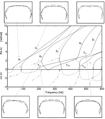
The dispersion relationship is determined for an undamped case for the sake of clarity. Figure 2 shows the polar wavenumber (rad/rad) below 600Hz for modes where the tread motion is predominantly in the plane of the tyre cross-section and not in the circumferential direction. Results for real, imaginary and complex (conjugates) wavenumbers are shown. Complex conjugate wavenumbers are only plotted close to their cut-off frequencies for clarity. Natural frequencies occur if Re(k_{)=1,2,··· and also if Re(}k_{)=0 for the purely breathing modes [9] although}

they do not occur in the frequency range shown for the tyre model.

The anti-symmetric A1 mode cuts-on first. This comprises the side-to-side motion of the tread as

illustrated in the figure. In the illustrations of wave modes, the solid line is the original shape and the dashed line is the deformed shape. The A1 and symmetric S1 wave modes are bouncing

modes where the belt mass is vibrating on the sidewall stiffness. The A2, S2 wave modes are

typical cross-sectional modes. Curve veering between two wave modes implies that the two wave modes are not orthogonal, and the deformed shape in general changes with frequency.

Negative group velocity can be observed especially for lower order wave modes. As the imaginary part of the complex conjugate wavenumbers becomes zero, two waves cut-on with a nonzero real wavenumber. One wavenumber increases with frequency while the other decreases implying a negative group velocity. The wave associated with the negative group velocity becomes a pure nearfield (with imaginary wavenumber) as frequency increases, and cuts-on again as a predominantly shear wave. The wave mode shapes change relatively rapidly with frequency, as the wave modes for TS1 at different frequencies illustrate. Above about

-0.1 0 0.1

0.2 0.25 0.3 0.35

-0.1 0 0.1

0.2 0.25 0.3 0.35

0 100 200 300 400 500 600

-4 -2 0 2 4 6 8 10 Frequency [Hz] -I m | k | R e | k | [ ra d /r a d ]

-0.1 0 0.1 -0.1 0 0.1 0.2

0.25 0.3 0.35

-0.1 0 0.1

[image:5.595.116.485.68.484.2]

Figure 2.-Relationship between frequency and the polar wavenumber: ―: real, ····: imaginary, −·−: complex conjugate wavenumbers. Anti-symmetric (Ai) and symmetric (Si) wave modes,

i_=1,2,3.T_{i denotes shear wave modes.}

4.4 Forced response

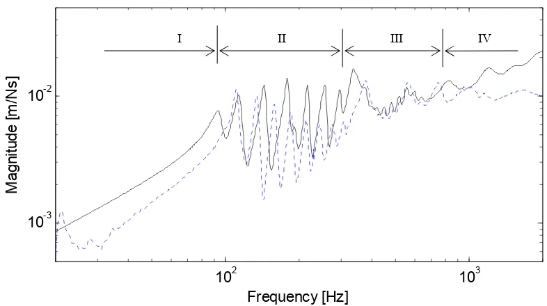
The input mobility at the centre of the tread is calculated using the formulation of (Eqs. 7). For a point force excitation, only symmetric modes are then excited. The frequency dependent loss factor (Eq. 11) is now included in

K

_rubber. All wavenumbers become complex because of the damping. Figure 3 shows the magnitude of the predicted and measured mobility. The experiment was performed in a freely supported condition using rubber strings such that the response below 30Hz is dominated by the boundary conditions. Good agreement can be seen on the whole. It should be noted that only about 70 pairs of positive- and negative-going wave modes are used to extract the numerical result. This implies that only 140 DOFs can express the dynamic behaviour of the tyre model below 2kHz.

The response may be characterised by four frequency regions, i.e. (I) below the first resonance (at which the S1 mode cuts-on) where the sidewall stiffness dominates the system motion, (II)

between the first resonance and the frequency where the S2 mode cuts on, in which the

response is like that of a beam on a flexible foundation, (III) at middle frequencies where the response is somewhat constant and plate-like and (IV) at high frequencies where the response is similar to that of an elastic half space. However, the experiment shows more or less a flat response even at high frequencies. Possible reasons for this are as follows. In the experiment, the excitation area is finite (a circular area of diameter 23.5mm is excited) so that higher order

wave modes cannot be properly excited. In addition, there is a resonance of the experimental rig around 4kHz, which could contaminate the result. Agreement at low and middle frequencies could be improved by updating the FE model parameters.

10

2

10

3

10

-3

10

-2

Frequency [Hz]

M

a

g

n

it

u

d

e

[

m

/N

s

[image:6.595.100.493.121.341.2]

]

Figure 3.-Magnitude of the Input mobility at the centre of the tread; ―: the WFE result, ····: experiment.

5. CONCLUSIONS

The wave finite element (WFE) method has been applied to a tyre, including the frequency dependent material properties. The free and forced vibration of the tyre was determined. The FE model of a short section of the tyre was formed using the commercial package ANSYS and subsequently post-processed. The model had only 324 DOFs. Geometrical and structural details were included. Only 70 wave mode pairs (140 DOFs) were retained to predict the forced response. The dispersion relationship was found including nearfield waves and complex wave behaviour was observed. The forced response was determined by the wave approach in conjunction with a numerical implementation, which is always well-conditioned. Good agreement with experimental data was seen. It can be concluded that the WFE method is a powerful tool to investigate the dynamic behaviour of a complex structure with small calculation cost.

ACKNOWLEDGEMENT

The authors gratefully acknowledge Bridgestone Corporation for providing the tyres and material data.

References: [1] U. Sandberg, J.A. Ejsmont: Tyre/Road Noise Reference Book. Informex (2002).

[2] D. Duhamel, B.R. Mace, M.J. Brennan: Finite element analysis of the vibrations of waveguides and periodic structures. Journal of Sound and Vibration 294 (2006) 205-220.

[3] B.R. Mace, D. Duhamel, M.J. Brennan, L. Hinke: Finite element prediction of wave motion in structural waveguides. Journal of the Acoustical Society of America 117,5 (2005) 2835-2843.

[4] S. Finnveden: Evaluation of modal density and group velocity by a finite element method. Journal of Sound and Vibration 273 (2004) 51-75.

[5] W. Kropp, K. Larsson, F. Wullens, P. Andersson: High frequency dynamic behaviour of smooth and patterned passenger car tyres. Proceedings of the Institute of Acoustics 26,2 (2004) 1-12.

[6] W.X. Zhong, F.W. Williams: On the Direct Solution of Wave Propagation for Repetitive Structures. Journal of Sound and Vibration 181,3 (1995) 485-501.

[7] Y. Waki, B.R. Mace, M.J. Brennan: On Numerical Issues for the Wave/Finite Element Method. ISVR Technical Memorandum No:964 (2006).

[8] W.M. Madigosky, G.F. Lee, J.M. Niemiec: A method for modeling polymer viscoelastic data and the temperature shift function. Journal of the Acoustical Society of America 119,6 (2006) 3760-3765.

[9] Y.J. Kim, J.S. Bolton: Modeling of Tire Treadband Vibration. internoise 2001, Hague (2001) 2605-2610.