Numerical solution of Fokker-Planck equation using the integral radial basis function networks

NUMERICAL SOLUTION OF FOKKER-PLANCK EQUATION USING THE INTEGRAL RADIAL BASIS FUNCTION NETWORKS

C.-D. Tran1, N. Mai-Duy1, T. Tran-Cong1

1 _{Computational Engineering and Science Research Centre (CESRC), Faculty of} Engineer-ing and SurveyEngineer-ing, University of Southern Queensland, Toowoomba, QLD 4350, Australia ([email protected])

Abstract. The Fokker Planck Equation (FPE) is a partial differential equation for the prob-ability density and transition probprob-ability of a random process. Owing to its broad range of applications, the FPE has been an interesting research topic. Recently, Radial basis functions (RBFs) have emerged as a powerful numerical tool for solving partial differential equations and this paper reports an integrated RBFs (IRBFs) based numerical method for the solution of FPEs. The use of integration to construct RBF approximants helps avoid the reduction in con-vergence rate caused by differentiation [1]. Numerical experiments showed that IRBF methods can yield accurate solutions on a much coarser mesh, thus reducing the computational effort required for a given degree of accuracy.

Keywords: Fokker-Planck Equation, Parabolic partial differential equation, Integrated Radial Basis Functions, Collocation point.

1. INTRODUCTION

The Fokker-Planck Equation (FPE) is used to describe a stochastic process in diverse fields, including plasma physics, biophysics, engineering, neurosciences, nonlinear hydrody-namics, and polymer physics. The FPE is a partial differential equation for the probability density and transition probability of such random processes. Owing to its broad range of ap-plications, the FPE has attracted significant attention of several researchers.

approach [10], various improvements can be made for solving larger problems. For example, one can improve the condition number of the system matrix by a localisation of the RBF ap-proximants [11] or domain composition techniques [12]. More recently, numerical schemes, based on the integrated RBFs (IRBFs) approach, for solving differential differential equations were reported [1, 13]. The use of integration to construct the RBF approximants is expected to overcome the problem of reduced convergence rate caused by differentiation [1]. Numerical experiments showed that IRBF based methods can yield accurate solutions on a coarse mesh [13], and thus have the ability to reduce the computational effort required for a given degree of accuracy. In this work, we present a collocation technique incorporating the one dimensional integrated RBFs (1D-IRBF) for a numerical solution of FPEs.

The paper is organized as follows. Section 2 gives a short review of several forms of the FPEs. In section 3, the discretization of a FPE using the 1D-IRBF method is detailed. Several numerical examples are then discussed in section 4 with a conclusion in section 5.

2. THE FOKKER PLANCK EQUATION

Consider the FPE for a field variableu(x, t)of 1–D independent variablesxand timet

as follows [2].

∂u(x, t)

∂t =

− ∂

∂xA(x) + ∂2

∂x2B(x)

u(x, t) (1)

whereA(x)> 0is the drift coefficient;B(x) >0the diffusion coefficient. The initial condi-tion is given by

u(x,0) =f(x), x∈ ℜ (2)

wheref(x)is a known function. If the drift and diffusion coefficients depend on time, Eq. (1) is expressed as

∂u(x, t)

∂t =

− ∂

∂xA(x, t) + ∂2

∂x2B(x, t)

u(x, t) (3)

In certain applications, the drift and diffusion coefficients are dependent on the distribution functionu(x, t)itself and the FPE can be expressed (see [2, 4] for details) by

∂u(x, t)

∂t =

− ∂

∂xA(x, t, u) + ∂2

∂x2B(x, t, u)

u(x, t) (4)

Generally, Eq. (4) for a vector variablex_{= (x1, x2, ..., xn)}T _{is rewritten as}

∂u(x_{, t)}

∂t =

"

− n

X

i=1

∂ ∂xi

Ai(x, t, u) + n

X

i,j=1

∂2

∂xixj

Bi,j(x, t, u)

#

u(x_{, t) (5)}

Mathematically, FPE is a second–order parabolic partial differential equation (more details can be found in [2]). In the next sections, a 1D-IRBF based computational technique is described for the numerical solution of FPEs.

3. 1D-IRBF MESHFREE METHOD FOR THE SOLUTION OF FPEs

3.1. 1D-IRBFs for a time dependent function

At a given time t, the highest-order derivative of the dependent variable u(x, t) (the second order for a FPE) is decomposed as

∂2_{u(x, t)}

∂x2 =

Nx X

i=1

wi(t)G[2]_i (x), (6)

where{wi(t)}Nx

i=1is the set of RBF weights;{G [2] i (x)}

Nx

i=1the set of Multi-quadric RBFs (MQ-RBFs), generally considered as one of the best RBFs for the approximation of a function [14], and given by

G[2]_i (x) = (x−ci)2+a2_i1/2, (7)

where{ci}Nx

i=1 is a set of centres and{ai}N

x

i=1a set of MQ-RBF widths [15].

The corresponding first-order derivative and the function itself are then determined through integration as follows.

∂u(x, t)

∂x =

Nx X

i=1

wi(t)G[1]_i (x) +C1(t), (8)

u(x, t) = Nx X

i=1

wi(t)G[0]_i (x) +C1(t)x+C2(t), (9)

whereG[1]_i (x) =R G[2]_i (x)dx,G_i[0](x) =R G[1]_i (x)dxandC1andC2are unknown constants of integration at timet.

Collocating equations (6), (8) and (9) at a set of grid points{xi}Nx

i=1yields the following set of algebraic equations

∂2_{eu(x, t)}

∂x2 =Ge

[2]_{(x)we(t), (10)}

∂u_{e(x, t)}

∂x =Ge

[1]_{(x)we(t), (11)}

e

u_{(x, t) =}Ge[0]_(x)w_{e(t), (12)} where

e

G[2] ₌

    

G[2]₁ (x1) G[2]2 (x1) · · · G [2]

Nx(x1) 0 0 G[2]₁ (x2) G[2]2 (x2) · · · G[2]Nx(x2) 0 0

..

. ... . .. ... ... ...

G[2]₁ (xNx) G

[2]

2 (xNx) · · · G

[2]

Nx(xNx) 0 0     , e

G[1] ₌

    

G[1]₁ (x1) G[1]₂ (x1) · · · G[1]_Nx(x1) 1 0 G[1]₁ (x2) G[1]₂ (x2) · · · G[1]_Nx(x2) 1 0

..

. ... . .. ... ... ...

G[1]₁ (xNx) G

[1]

2 (xNx) · · · G

[1]

Nx(xNx) 1 0     , e

G[0] ₌

    

G[0]₁ (x1) G[0]2 (x1) · · · G[0]Nx(x1) x1 1 G[0]₁ (x2) G[0]2 (x2) · · · G

[0]

Nx(x2) x2 1

..

. ... . .. ... ... ...

G[0]₁ (xNx) G

[0]

2 (xNx) · · · G

[0]

e

w_{(t) = (w1(t), w2(t),· · ·, wNx(t), C1(t), C2(t))}T _,

e

u_{(x, t) = (u1(x, t), u2(x, t),· · ·, uNx(x, t))}T _,

dk_{ue(x, t)}

dxk =

dk_{u1(x, t)}

dxk ,

dk_{u2(x, t)}

dxk ,· · ·,

dk_u

Nx(x, t) dxk

T

,

whereui =u(xi, t)withi= (1,2,· · ·, Nx).

Owing to the presence of integration constants in the IRBF based approximants, one can beneficially introduce in the algebraic equation system additional constraints such as nodal derivative values (more details can be found in [13, 1]). Thus, the algebraic equation system (12) can be reformulated as follows.

e u ef = " g G[0] e L # e

w₌Cew_e,

whereef ₌Lew_{e are additional constraints. The conversion of the network-weight space into the} physical space yields

e

w₌Ce−1

e u ef , (13) e

C−1 _{is the conversion matrix. By substituting (13) into (6) and (8), the second and first-order} derivatives ofu(x, t)will be expressed in terms of nodal variable values as follows.

∂2_u(x,t)

∂x2 =D2xu˜(x, t) +k2x,

∂u(x,t)

∂x =D1xu˜(x, t) +k1x,

(14)

whereD1x andD2x are known vectors of lengthNx; andk2xandk1x scalars. Applying (14) at each and every collocation point yields

∂2_eu(x,t)

∂x2 =De2xu˜(x, t) +ek2x,

∂eu(x,t)

∂x =D1xe u˜(x, t) +ek1x,

(15)

where D2xe and D1xe are known matrices of dimensionNx ×Nx; and ek2x and ek1x are known vectors of lengthNx.

3.2. Temporal and spatial discretization of FPEs

The FPE (1),(x, t)∈Ω×[0, T], is rewritten as follows

∂u ∂t −B

∂2u ∂x2 +

A−2∂B

∂x ∂u ∂x + ∂A ∂x −

∂2B ∂x2

u= 0, (16)

wherex,t,u(x, t),A(x)andB(x)are defined as before.

Assume that the time interval[0, T]is partitioned intonT equal subintervals[tn, tn+1]of length∆t=T /nT witht0 = 0andtNT =T. In fully discrete schemes, Eq. (16) is discretized

with respect to both time and space variables. The discretization in time is accomplished by a time-stepping scheme, followed by the spatial discretization based on the 1D-IRBFN method.

Applying theθ-scheme to Eq. (16) yields

un+1_−un

∆t +θLu

wheretn+1 _=tn_{+ ∆t,u}n+1 _{=u(x, t}n+1_{)and the operatorLis given by}

L(.) = −B∂

2_(.)

∂x2 +

A−2∂B

∂x

∂(.)

∂x +

∂A

∂x −

∂2_B

∂x2

(.). (18)

For the Crank-Nicolson method (θ = 0.5 and second-order accurate), Eq. (17) is expressed as

un+1+αLun+1 =un−αLun, (19)

whereα = 0.5∆t.

For the fully implicit method (θ = 1), Eq. (17) is rewritten as

un+1+αLun+1 =un, (20)

whereα = ∆t.

For the fully explicit method (θ = 0), Eq. (17) is given by

un+1 =un−αLun, (21)

whereα = ∆t.

Equations (19)-(21) together with the constraints (boundary or/and initial conditions) at time tn+1 _{are then spatially discretized using the 1D-IRBF approach described in section} 3.1. The obtained solution is the values of the field variable at the grid points. Simulation is terminated when either the desired time (transient problem) or convergence (steady state problem) is reached. In the next section, the fully implicit method is used for time discretization of the FPEs.

4. NUMERICAL EXAMPLES

The present method is verified with some numerical experiments which have been de-scribed in [4, 16, 17]. It is worth noting that the problems are solved on a bounded interval which is uniformly discretized. The approximate solutions obtained are compared with the analytic ones using the following error norms

Ne =

sPN

i=1(un(xi)−uex(xi)) 2

PN

i=1(uex(xi))2

RMSE =

s_P

N

i=1(un(xi)−uex(xi)) 2

N

whereu(xi), uex(xi)are the numerical and exact solutions foru respectively at a collocation pointxi and timetnandN the total number of test points.

4.1. Example 1

Consider the FPE (1)

∂u(x, t)

∂t =

− ∂

∂xA(x) + ∂2

∂x2B(x)

0 0.1 0.2 0.3 0.4 0.5 0.6 0.7 0.8 0.9 1 10−15

10−14 10−13 10−12 10−11 10−10

x

error

t = 1.0 t = 0.5 t = 0.1

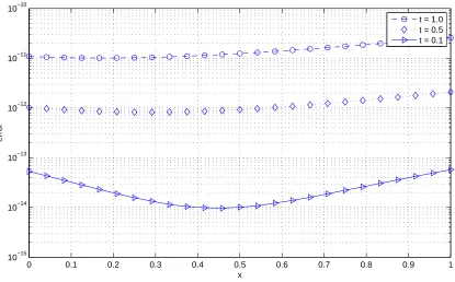
Figure 1. The absolute error ofuwith respect toxat timest= 0.1,t= 0.5andt = 1.

withA(x) = −1, andB(x) = 1 and initial conditionu(x,0) = x, (x ∈ [0,1]). The exact solution to the problem isu(x, t) =x+t.

The problem is solved in the time period[0,1]with time step size ∆t = 0.01. Figure 1 shows the error ofuwith respect toxat timest = 0.1,t = 0.5andt = 1 using the present method with25collocation points in comparison with the exact solution.

The problem is also solved using15and36collocation points. The values ofNe and RMSE using 50 test points with 15, 25 and 36collocation points are given in table 1. The results show that the method yields a higher degree of accuracy while using relatively coarse grids in comparison with others, including the Kansa RBF (table 2) and Hermite RBF (table 3) approaches.

Table 1. Values ofNeandRMSEfor numerical examples 1,2,3 for several sets of collocation points (15, 25 and 36) using the 1D-IRBF collocation method. The number of test points is

N = 50and∆t= 0.01.

Example 1 Example 2 Example 3

N Ne RMSE Ne RMSE Ne RMSE

15 3.45e−6 1.16e−6 3.62e−4 6.74e−4 4.16e−4 7.86e−4 25 8.25e−7 2.89e−7 2.22e−5 3.54e−5 9.28e−6 1.13e−5 36 5.48e−9 1.94e−9 7.62e−7 2.37e−7 5.12e−7 6.38e−7

4.1.1 Example 2

Consider the Fokker-Planck equation (1) with

A(x) =x, B(x) = x 2

0 0.2 0.4 0.6 0.8 1 1

1.5 2 2.5 3 3.5 4 4.5 5 5.5

x

u

t = 0.1 t = 0.5 t = 1

exact solution

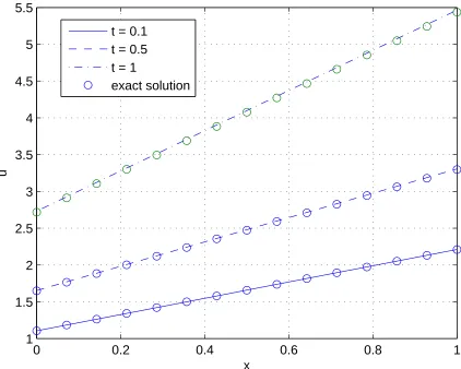
Figure 2. Exact and approximate solutions foruare plotted againstxat timest= 0.1,t= 0.5 andt = 1.

t ∈ [0,1],x ∈[0,1], and initial conditionu(x,0) =f(x) =x. The exact solution is given by

u(x, t) =xexp(t).

Similarly, the problem is solved with time step size∆t = 0.01and three sets of col-location points as in example 1. Errors are shown table 1 using 50 test points as in example 1. A comparison with the other results given in tables 2 and 3 confirms higher accuracy of the present solution.

4.1.2 Example 3

Consider the backward Kolmogorov FPE (see [2] for more details) as follows

∂u(x, t)

∂t =−

A(x, t) ∂

∂x +B(x, t) ∂2

∂x2

u(x, t) (24)

where the drift and diffusion coefficients depend on both time and space as follows

A(x, t) =−(x+ 1), B(x, t) =x2exp(t). (25)

With the initial condition

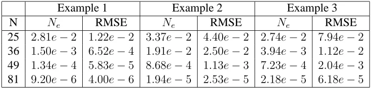
Table 2. Values ofNeandRMSEfor numerical examples 1,2,3 for several sets of collocation points (25, 36, 49 and 81) using the Kansa’s RBF approach,∆t= 0.01and the number of test pointsN = 50. Data are obtained from source [16]

Example 1 Example 2 Example 3

N Ne RMSE Ne RMSE Ne RMSE

25 2.81e−2 1.22e−2 3.37e−2 4.40e−2 2.74e−2 7.94e−2 36 1.50e−3 6.52e−4 1.91e−2 2.50e−2 3.94e−3 1.12e−2 49 1.34e−4 5.83e−5 8.68e−4 1.13e−3 7.23e−4 2.04e−3 81 9.20e−6 4.00e−6 1.94e−5 2.53e−5 2.18e−5 6.18e−5

Table 3. Values ofNeandRMSEfor numerical examples 1,2,3 for several sets of collocation points (25, 36, 49 and 81) using the Hermite RBF without time discretization scheme. The number of test points isN = 50. Data are obtained from source [16].

Example 1 Example 2 Example 3

N Ne RMSE Ne RMSE Ne RMSE

25 1.48e−4 6.41e−5 2.12e−4 1.21e−4 1.73e−4 2.23e−4 36 2.30e−5 9.92e−6 7.11e−5 5.43e−5 1.13e−4 1.61e−4 49 2.81e−6 1.21e−6 8.63e−6 6.86e−6 8.29e−5 8.61e−5 81 3.83e−8 1.65e−8 4.93e−8 3.12e−8 1.35e−7 1.76e−7

the exact solutionto the problem isu(x, t) = (x+ 1) exp(t).

Figure 2 shows the approximate solution with respect toxusing a very coarse grid of 15collocation points at times t = 0.1, t = 0.5 andt = 1. The problem is also solved with 25 and 36 collocation points. Similar comments as in examples 1 and 2 can be made here regarding results in tables 1, 2 and 3.

In general, although the accuracy of solutions tends to decrease with time, the results claimed that the present method can reach high order accuracy using coarse grids.

5. CONCLUSION

The 1D-IRBF based meshfree method has been successfully developed for the com-putation of FPEs. The advantages of the present approach include (i) to yield a meshless discretisation of FPEs; (ii) to improve the approximation accuracy by avoiding the reduction in convergence rate caused by differentiation; (ii) to reduce the noise in the approximation via the use of integration as a smoothing operator to construct the approximants. The present method is demonstrated with several forms of FPEs. The obtained results show that the present method yields a high degree of accuracy with relatively coarse grids.

Acknowledgements

6. REFERENCES

[1] Mai-Duy N., Tran-Cong T., “Numerical solution of differential equations using multi-quadric radial basis function networks”. Neural Networks 14, 185-199, 2001.

[2] Risken, H., “The Fokker-Planck equation: method of solution and applications”, 1989, Springer Verlag Berlin.

[3] Zorzano M. P., Mais H., Vazquez L., “Numerical solution of two-dimensional Fokker-Planck equations”. Appl. Math. Comput. 98, 109-17, 1999.

[4] Dehghan M., Tatari M., “The use of He’s variational iteration method for solving a Fokker-Planck equation”. Phys. Scr. 74, 310-6, 2006.

[5] Odibat Z., Momani S., “Numerical solution of Fokker-Planck equation with space and time fractional derivatives”. Phys. Lett. A 369, 349358, 2007.

[6] Harrison G. Numer. Meth. “Numerical solution of the Fokker-Planck equation using moving finite elements”. Part. Diff. Eqs. 4, 219-32, 1988.

[7] Jafari M. A., Aminataei A. “Application of homotopy perturbation method in the solution of Fokker-Planck equation”. Phys. Scr. 80, 055001, 2009.

[8] Fasshauer G. E., Meshfree approximation methods with Matlab (Interdisciplinary Math-ematical Sciences Vol. 6, World Scientific, Singapore, 2007.

[9] Kansa E., “Multiquadrics a scattered data approximation scheme with applications to computational fluid dynamics-I: Surface approximations and partial derivatives esti-mates”. Computers & Mathematics with Applications 19, 127145, 1990.

[10] Kansa E. J., “A scattered data approximation scheme with applications to computational fluid-dynamics. II. Solutions to parabolic, hyperbolic and elliptic partial differential equa-tions’. Comput. Math. Appl. 19, 147-161, 1990.

[11] Sarler B., Vertnik R., “Meshfree explicit local radial basis function collocation method for diffusion problems”. Comput. Math. Appl. 51, 1269-1282, 2006.

[12] Divo E., Kassab A., “Iterative domain decomposition mesh-less method modeling of in-compressible viscous flows and conjugate heat transfer”. Eng. Anal. Boundary Elements 30, 465-478, 2006.

[13] Mai-Duy N., Tran-Cong T., “A Control Volume Technique Based on Integrated RBFNs for the Convection-Diffusion Equation”. Numerical methods for partial differential equa-tions 26, 426447, 2010.

[14] Franke R., “Scattered data interpolation: tests of some methods”. Mathematics of Com-putation 38, 181200, 1982.

[15] Haykin S., Neural networks: A comprehensive foundation. New Jersey:Prentice Hall, 1999.

[16] Kazem S., Rad J. A., Parand K., “Radial basis functions methods for solving Fokker-Planck equation”. Engineering Analysis with Boundary Elements 36, 181-189, 2012. [17] Tatari M., Dehghan M., Razzaghi M., “Application of the Adomian decomposition