Single-shot time-gated fluorescence lifetime imaging using three-frame images

Single-shot time-gated fluorescence lifetime imaging

using three-frame images

Yahui Li1,2,3, Hui Jia3, Shaorong Chen3,5, Jinshou Tian1,2,6, Lingliang Liang3, Fenfang Yuan3, Hongqi Yu3, David Day-Uei Li4,7

1_{Key Laboratory of Ultra-fast Photoelectric Diagnostics Technology, Xi’an Institute}

of Optics and Precision Mechanics, Xi’an, Shanxi 710049, China

2_{University of Chinese Academy of Sciences, Beijing 100049, China} 3_{Laboratory of Ultra-fast Imaging, College of Electronic Science and Engineering,}

National University of Defense Technology, Changsha, Hunan 410073, China

4_{Faculty of Science, University of Strathclyde, Glasgow G4 0RE, Scotland, UK} 5_{[email protected]}

6 _{[email protected]} 7_{[email protected]}

OCIS codes: (110.4155) Multiframe image processing; (170.3650) Lifetime-based sensing; (170.6920) Time-resolved imaging; (280.2490) Flow diagnostics; (300.2530) Fluorescence, laser-induced.

Abstract

Qualitative and quantitative measurements of complex flows demand for fast

single-shot fluorescence lifetime imaging (FLI) technology with high precision. A method, single-shot time-gated fluorescence lifetime imaging using three-frame images (TFI-TGFLI), is presented. To our knowledge, it is the first work to combine a three-gate rapid lifetime determination (RLD) scheme and a four-channel framing camera to achieve this goal. Different from previously proposed two-gate RLD schemes, TFI-TGFLI can provide a wider lifetime range 0.6 ~ 13ns with reasonable precision. The performances of the proposed approach have been examined by both Monte-Carlo simulations and toluene seeded gas mixing jet diagnosis experiments. The measured average lifetimes of the whole excited areas agree well with the results obtained by the

streak camera, and they are 7.6ns (N2 = 7L/min; O2 < 0.1L/min) and 2.6ns (N2 =

19L/min; O2 = 1L/min) with the standard deviations of 1.7ns and 0.8ns among the

experimental settings.

1. Introduction

Planar laser-induced fluorescence (PLIF) sensing technologies are widely used in many scientific fields, such as airflow, combustion, and plasma diagnostics [1] due to its ability to measure the concentration, temperature, pressure and velocity [2, 3]. Compared to other diagnostic techniques such as coherent anti-Stokes Raman scattering (CARS) or tunable diode laser absorption spectroscopy (TDLAS), the advantage of

PLIF is the ability to perform two-dimensional (2D) sliced wide-field imaging by shaping the excitation light into a light sheet [4]. Although the fluorescence signals carry the information about the concentrations of the probed species, it is challenging to conduct qualitative and quantitative measurements – multiple parameters need to be confirmed in order to either relatively compare or precisely obtain the species concentrations [5]. It is a challenging task to accurately assess the fluorescence quantum yield that is affected by collisions, simulated emissions, predissociations, and photoionizations. It is difficult to assess the impact of the collisional quenching in collisional processes, since the quenching depends on temperature, pressure, and

quenchers, making PLIF only suitable for flow visualization. For example, OH-PLIF, CH2O-PLIF, and CH-PLIF are used respectively to observe the reaction, preheating and

heat releasing zones in a combustion field [6]. Accurately assessing the collisional quenching rate is the main key to achieving qualitative and quantitative measurements. The collisional quenching rate can be directly determined by measuring the fluorescence lifetime. The fluorescence lifetime measurement techniques can be divided into time-domain and frequency-domain methods [7]. In time-domain methods [8], such as time-correlated single-photon counting (TCSPC) [9 ~ 11] and time-gated FLI [12 ~ 14], the fluorescence intensity decay is measured with pulsed laser excitations.

For non-repetitive dynamic events in complex flows and combustions, we expect

to obtain the fluorescence lifetime images with a single excitation to freeze the instantaneous structures. Conventional time-gated FLI measures the fluorescence delay functions by gating the image intensifier of an ICCD camera with different delays. It usually needs to acquire more than one time-gated shot. Single-shot lifetime measurements can be achieved by replacing the single ICCD camera with two or more ICCD cameras to take time-resolved images simultaneously. Omrane et al. measured phosphorescence images with a high-speed framing camera containing eight independent ICCD image detectors, their system can obtain lifetimes in the order of milliseconds using an exponential fitting procedure [18]. However, this method is not

suitable for measuring lifetimes around nanoseconds in a single shot. Ehn. et al.

presented a single-shot FLI method with PLIF, using a dual ICCD detection setup with different gating characteristics for the two cameras, and they successfully demonstrated real-time acquisition of formaldehyde in a premixed, laminar methane/oxygen flame. The measured lifetimes range from 1.0 to 4.5ns [19].

The most traditional approach for lifetime estimations is to acquire a multipoint decay curve and analyze it with least-square methods. This approach, however, requires considerable acquisition and computational time and is therefore unsuitable for single-shot time-gated FLI. The rapid lifetime determination (RLD) method was previously proposed to allow analyzing the decay data in real-time. For single-exponential decays,

the lifetimes can be easily evaluated. RLD is suitable for single-shot time-gated FLI, if two ICCD cameras are used. RLD has a variety of gating schemes [14, 20], such as the standard RLD (SRLD) using two gates of the same width or other more optimized RLD (ORLD) approaches. We can select a proper gating scheme to achieve a certain lifetime measurement range. In 2012, Ehn et al. achieved single-shot FLI of a toluene seeded gas mixture jet [21] using the same experimental setup as their earlier work [19], and they presented an evaluation algorithm, DIME (Dual Imaging and Modeling Evaluation), based on an ORLD scheme to evaluate image data. They estimated the lifetimes around 800ps with a standard deviation around 120ps (from 100 repeated

of the oxygen concentration in toluene/nitrogen/oxygen mixtures. The results agreed

with the Stern-Volmer model, showing the potential for detecting the oxygen concentration through fluorescence lifetime measurements. Monte-Carlo simulations were performed to evaluate the sensitivity of DIME for oxygen detection. The results indicated a high measurement sensitivity in the range 0.5 ~ 6mol/m3 [22], showing that DIME has potential for quantitative diagnosis of complex flows. However, traditional RLD methods have a drawback: they are unable to offer robust estimations if the samples to be tested have a wide range of lifetimes. In order to solve this problem, Ehn

et al. also proposed an approach that the measurement precision is virtually insensitive to the lifetime with ramped gain functions for the two ICCD cameras. However, this

solution requires extra modifications on the driving front-ends to generate the ramped gain function, which might be challenging to achieve.

We described an approach named ‘single-shot time-gated fluorescence lifetime imaging using three-frame images (TFI-TGFLI)’ to provide high-speed, high-precision and wide dynamic range (0.6 ~ 13ns) FLI. In this paper, we will firstly demonstrate the relationships between the fluorescence lifetimes and the quencher concentrations and the relationships between the pre-exponential factors and the fluorophore concentrations using the simple two-state fluorescence emission model. The TFI-TGFLI experimental setup will then be described. Secondly, we will introduce the lifetime (and pre-exponential factor) determination algorithm for TFI-TGFLI and will

show the Monte-Carlo simulation results. Finally, the experimental results will be presented with the image data processed and analyzed to obtain the fluorescence lifetime images and the normalized fluorophore concentration images in two toluene-seeded gas mixing jets: 1) N2 = 7L/min, O2 < 0.1L/min (denoted as N2:O2 > 7:0.1

hereafter for simplicity), and 2) N2 = 19L/min, O2 = 1L/min (denoted as N2:O2 = 19:1

hereafter). The results will also be compared with those obtained from a streak camera.

2. Theory and experimental setup

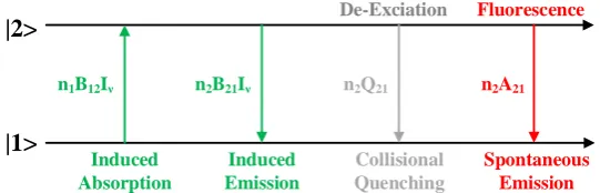
Figure 1 shows a two-state system model of a fluorescent molecule [23]. The

n1 and n2 are the concentrations at the states |1> and |2>. B12，B21，Q21 and A21are the

stimulated absorption, stimulated radiation, collisional quenching (non-radiation) and spontaneous emission probabilities, respectively. Iν is the intensity of the laser pulse in absorption lines. The rate equation at the state |2> can be expressed as

 

 



 



2 1 12 2 21 21 21

n t n t I B_ n t I B_ Q A ， (1)

After the excitation, i.e. Iν= 0,

n t

 



n

exp









Q



A t







concentration at the state |2> after the excitation. Because the fluorescent signal is the spontaneous emission from the state |2>, the time resolved signal Nf can be derived as

 

 





4

f c

N t VA n t A t 





   , (2)

where,





21 2 , =1 21+ 21

4

AE c

A VA n  A Q





 , (3)

Ω is the solid angle for detection and V is the exited volume. ηc is the quantum efficiency

of the collection optical system including a UV lens and a filter. Due to A21<< Q21, τ ≈ 1/Q21.

Under the weak excitation limit (linear LIF), n2 << n1, Eq. (1) can be transformed

to n t₂

 





the states |1> before the laser excitation. Substituting 2 10





AE

n 



Eq. (3), the pre-exponential factor A can be written as

0 21 12 1

4 c

A VA B n I dt_









Therefore, n10 can be quantified by measuring A, which can be directly calculated from





exp

S





with the lifetime τ being measured and A21, B12, and Iν already known. S is the integrated fluorescent intensity over the exposure time. We can conclude that measuring τ and A

plays an important role in quantifying the concentrations of the quenchers and the

|2>

|1>

n1B12Iν n2B21Iν n2Q21 n2A21

Induced Absorption

Induced Emission

Collisional Quenching

Spontaneous Emission

De-Exciation Fluorescence

Fig. 1. Different transitions that are included in the two-state model.

The proposed TFI-TGFLI for estimating τ and A is to obtain three images in one

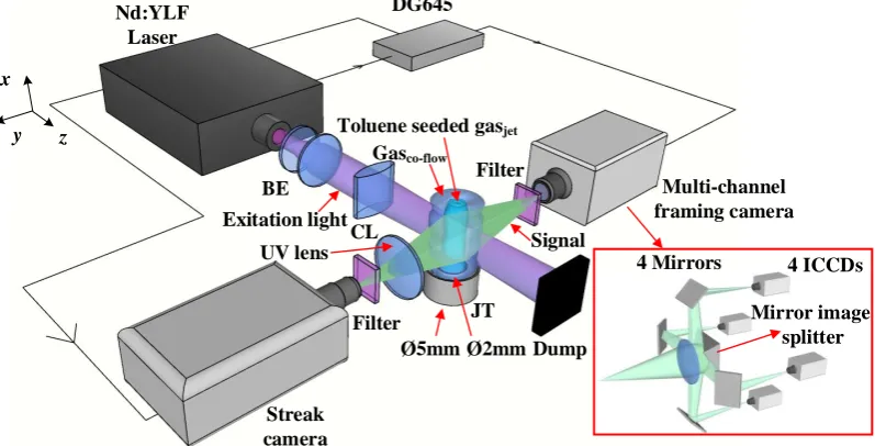
single shot by a multi-channel framing camera, and then estimating τ and A images via the Newton–Raphson method. The experimental setup is shown in Fig. 2. A fourth harmonic pulsed Nd:YLF laser (the central wavelength = 263.25nm; the pulse duration = 10ps; the energy per pulse = 2mJ; the repetition rate = 5Hz; the beam diameter = 6mm) was used. A beam expander (including a negative lens and a positive lens) was used to expand the laser beam, and a cylindrical lens was used to focus the laser beam in one dimension (y axis as shown in Fig. 2). A laser sheet was formed around the focus point of the cylindrical lens. In our experiments, the output laser beam was directly focused by the cylindrical lens (f = 500mm) into a laser sheet aligned with the probe

volume above a gas nozzle. The size of the laser sheet is 6mm×3mm (x×z). A

2mm-diameter jet tube (supplying toluene-seeded gas), was inserted at the center of a 5mm-diameter tube (providing a co-flow of gas shielding the central jet). The distance

between the jet tube and the Nd:YLF laser is ~ 0.6m. The Nd:YLF laser sent a triggering pulse to the digital delay generator DG645 to trigger both the streak camera and the four-channel framing camera (XXRapidFrame, Stanford Computer Optics) to respectively record the filtered fluorescent signals with 300nm longpass filters. The distance between the jet tube and the lens of the framing camera is ~1m. The diagram of the multi-channel framing camera is also shown in Fig. 2. In the inset, a mirror image splitter behind an imaging lens splits an image into four sub images. The exposure time of each channel can be controlled by the image intensifier of the ICCD. The streak camera was used to record 1-D decay curves the compare with the results of TFI-TGFLI.

(+x). And the measuring time window and scanning step are 40ns and 200ps,

respectively. We used a UV lens (f = 60mm, F/1.7) to gather the signal to the streak camera. Additionally, the distance between the jet tube and the slit of the streak camera is ~0.3m. The directions of the laser propagation and the gas jet are in +z axis and +x

axis, respectively.

x

y z

Nd:YLF Laser

DG645

Streak camera

Multi-channel framing camera

Dump Filter

Filter

JT CL

BE

Toluene seeded gasjet

Gasco-flow

Ø5mm Ø2mm Exitation light

UV lens _{4 Mirrors}

Mirror image splitter

4 ICCDs Signal

Fig. 2. Schematic illustration of the experimental setup. The laser beam is expanded through a beam expander (BE) and focused to a laser sheet by a cylindrical lens (CL) in the target area above the jet tubes (JT). A triggering pulse is sent to the digital delay

generator DG645 to trigger both the streak camera and the framing camera to record filtered signals. The multi-channel framing camera contains an image splitter and four

ICCDs.

3. The lifetime algorithm of TFI-TGFLI

This section describes the proposed three-gate rapid lifetime determination scheme, implemented on a newly developed four-channel framing camera to achieve single-shot FLI. We will compare its performance with an ORLD scheme [20].

exponential decay model, i.e. N_f

 





and we can neglect the IRFs in our experiments. To examine this, we have conducted Monte-Carlo simulations. The results show that the lifetime estimations with our proposed algorithm are indeed insensitive to the IRF for single-exponential analysis. In

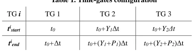
fact, gating approaches are in general less sensitive (compared with traditional TCSPC approaches) to the imperfections of the IRF for single-exponential analysis.The impact of the IRF in our instruments contributed to errors only around 3% (for τ = 0.6ns) and is therefore negligible in our discussions for simplicity. If the FWHM of the IRF is larger, we can time-shift the gate signal a bit away from the decay peak. This would sacrifice the photon efficiency a little bit, but for single-exponential analysis it is a well-known approach to reduce the bias [14, 24]. The orange, green, and purple areas represent three time-gates; their start times ti

start and end times tiend (i = 1, 2, and 3) are

listed in Table 1. TG represents ‘time-gate’.

t0+Y1Δt

Δt t0

TG 1

P1Δt

P2Δt t0+Y2Δt

10ps laser pulse

Intensity(a.u.)

t (ns)

0 0.2 0.4 0.6 0.8 1

10 20 30 40 50

0 1.2

TG 2

TG 3

Fig. 3. Graphical illustration of the three time-gates used to estimate lifetimes.

Table 1. Time-gates configuration

TG i TG 1 TG 2 TG 3

ti

start t0 t0+Y1Δt t0+Y2Δt ti

end t0+Δt t0+(Y1+P1)Δt t0+(Y2+P2)Δt

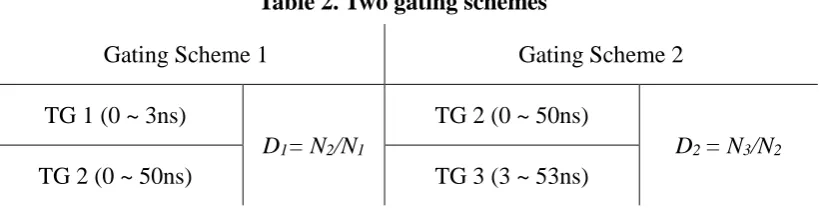
Table 2. Gating Scheme 1 consists of TGs 1 and 2; Gating Scheme 2 consists of TGs 2

and 3. The ranges in the parentheses represent the widths of the time-gates.The signal in TG i is

, ( 1, 2,3)

i end i start t

i _t i f

N 



k is the photoelectric conversion factor for the three channels, k ~ ηPCGMCPηpCηCCD, where ηPC is the quantum efficiency of the photocathode, GMCP is the gain factor of the microchannel plate, ηp is the quantum efficiency of the fluorescent screen, C is the coupling efficiency of the coupled optical system, and ηCCD is the quantum efficiency of the CCD, pi is the percentage of the total signal. Dj is the ratio of the signal Nj+1 to Nj,

(j=1,2). For TFI-TGFLI, the coefficients k for the ICCD cameras in the framing camera are similar, therefore the effects caused by the differences in the gain functions (time-dependent gain) can be neglected.

Table 2. Two gating schemes

Gating Scheme 1 Gating Scheme 2

TG 1 (0 ~ 3ns)

D1= N2/N1

TG 2 (0 ~ 50ns)

D2 = N3/N2

TG 2 (0 ~ 50ns) TG 3 (3 ~ 53ns)

To achieve single-shot acquisition based on three-gate RLD, a four-channel framing camera can be used to split a signal into four channels equally to obtain three images in Channels 1, 2, and 3 with TGs 1, 2, and 3 respectively. The signal collected in each channel would decrease to Ntot/4, i.e. pi= 25% (i = 1, 2, and 3); Ntot is the total number of the photons detected by the framing camera. In this work, we present

single-shot and wide dynamic-range FLI using three images (i = 1, 2 and 3), but we would also be able to fully use four images (i = 1, 2, 3 and 4) to improve the photon efficiency and to perform bi-exponential analysis in the future.

 

0

j

j j

j N

f D

N

 _  _{ }

, j = 1, 2.

The Newton iteration formula can be written as

   

, 1 , ,

'

,

0,1,2...,

1,2

j n j n

f

f

n

j

















where τj,0 is initial value of the iteration, with j = 1, 2 representing Gating Schemes 1 and 2. Applying Eq. (7) to all pixels, and two lifetime images, τ1 and τ2, can be obtained. Hence, two A images (A1 and A2) can also be obtained by Eq. (5).

To simplify the discussions, the technical details regarding the detectors were not considered. There are three types of noise in the signal obtained by the framing camera: shot noise, dark current noise and readout noise. Among them, shot noise is the

dominating factor to determine the signal-to-noise ratio (SNR). Therefore, we only consider the influence of the shot noise on the precision of the lifetime estimations. To quantify the performance of a lifetime determination scheme, we use the figure of merit introduced by Draaijer et al. [25] for the lifetime estimations. The definition is

 

F_  N 



 , (8)

στ is the standard deviation of τ, and hence στ/τ is the relative standard deviation. And,

the figure of merit FA can also be defined for A,

 

A tot

F A N

A



 , (9)

where σAis the standard deviation of A and σA/A is the relative standard deviation.Under a fixed Fi, (i = τ, A), increasing Ntot will improve the SNR of τ and A images. If Ntot is fixed, an FTI method with a larger Fi, (i = τ, A) has worse precision (larger relative standard deviation).

0.6 4.3 τ (ns) 0.6 2.6 τ (ns)

Fτ FA

0 5 10 15

2 4 6 8 10

0 5 10 15

2 4 6 8 10

2.7 1.3

(a) (b)

13

Gating Scheme 1

Gating Scheme 2

Enhanced Gating Scheme 1

ORLD Scheme

Gating Scheme 1

Gating Scheme 2

Enhanced Gating Scheme 1

Fig. 4. (a) Fτ and (b) FA curves as a function of τ for Gating Scheme 1 (blue line),

Gating Scheme 2 (red line), enhanced Gating Scheme 2 (dash blue line) and an ORLD scheme (Δt = 2ns, Y = 0, P = 200, black line).

Figures 4(a) and 4(b) show the Fτ and FA curves for Gating Schemes 1 (blue line), 2 (red line), enhanced Gating Scheme 1 (dash blue line) and an ORLD scheme (Δt = 2ns, Y = 0, P = 200, black line). For ORLD, two images are captured in a single shot by using two ICCD cameraspositioned in a right-angle configuration with a 70/30 beam splitter splitting the signal into two cameras as the DIME works [21]. TFI-TGFLI and OLRD optimize in different lifetime ranges. For TFI-TGFLI, as the number of images

acquired in a single-shot increases, the signal intensity of each image decreases, making the Fτ and FA curves of Gating Scheme 1 larger than ORLD. From the literature [22], the mole fraction of oxygen could vary between 1.64 and 8.36 mol/m3, the lifetime can vary between 0.7 and 3.0ns. It would be very useful for a FLI instrument to be able to resolve lifetimes in this range. TFI-TGFLI optimizes in the ranges, τ < 2.7ns for Fτ and

τ < 1.3ns for FA, whereas ORLD optimizes in a longer range. ORLD can be adjusted to

provide better sensitivity in a certain narrow range [20], whereas TFI-TGFLI can provide a more robust analysis if the lifetime varies significantly within the field of view.

The above simulation results show that we can simply take either τ1 or τ2 (similarly

A1 or A2) images according to the following equations,

 

 

_{ }

 

1

, , , 4.3

,

, ,

x z x z ns

x z

x z else

 





 

  

 , (10)

 

 

_{ }

 

1

, , , 2.6

,

, ,

A x z x z ns

A x z

A x z else



 

  

 . (11)

With Eqs. (10) and (11), we can obtain τ and A images with Fi (i = τ, A) < 6 for 0.6 < < 13ns and with high precision for 0.6 < < 2.7ns.

Although Channel 4 was not used in this work, it can be employed to enhance the photon efficiency in the future. If we set the time-gate of Channel 4 the same with that

Scheme 1 would be further improved. The Fτ and FA curves (dash blue lines) for the

enhanced Gating Scheme 1 is shown in Figs. 4(a) and 4(b). The other advantage of using multi-framing cameras is that we can expand our applications for bi-exponential analysis in the future.

The fluorescence lifetimes of a complex flow may vary significantly according to the temperature, pressure, or quencher concentration gradients. The proposed TFI-TGFLI can achieve single-shot acquisition, provide a wide dynamic range and improve the precision significantly in the short lifetime range, promising wider applications.

4. Analysis of the experimental results

The toluene seeded flows are consisted of N2 and O2 with different mixing ratios.

Two cases are demonstrated here; Case 1: N2:O2 > 7:0.1 (N2 = 7L/min; O2 < 0.1L/min.

The minimum significant digit that the flow meter can provide is 0.1L/min, therefore any rate lower than this value would indicate 0.0L/min. Thus, we tuned the meter of the O2 supply for Case 1 to 0.0L/min, but the actual flow rate should be < 0.1L/min) and

Case 2: N2:O2 = 19:1 (N2 = 19L/min; O2 = 1L/min). From the fluorescence lifetimes we

obtained in the experiments described below, we could conclude that the N2:O2 ratio

for Case 1 could be up to 120:1 whereas the measured lifetime  = 2.6ns for Case 2 is in a good agreement with the literature compared with the results reported in [22, 26]. The purpose of the experiments designed for this work is to evaluate the performances

of the proposed lifetime determination methods, and the experiments indeed confirm that the measurements obtained from the proposed camera are in good agreement with those obtained by the streak camera.

N2

:O

2

=

19:

1

1mm

x

z

x

z

x

z

x

z

x

z

x

z

Channel 1

Channel 1 Channel 2

Channel 2 Channel 3

Channel 3

0 0.5 1

0 0.5 1

N2

:O

2

<

7

:0.

1

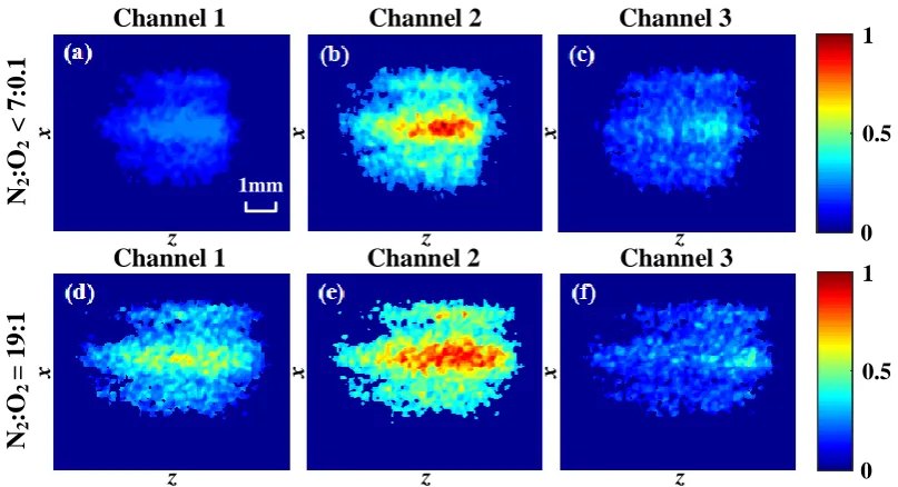
Fig. 5. Normalized fluorescent intensity images captured by the three channels of the framing camera for Case 1 (N2:O2 > 7:0.1), (a), (b), and (c), and Case 2 (N2:O2 =

19:1), (d), (e), and (f).

τ and A images can be calculated from the three intensity images shown in Fig. 5

using the lifetime determination algorithm mentioned in Section 3. In order to visualize the distributions of the toluene molecules, the intensity profile of the pulsed laser Iν

should be confirmed. We assume that the intensity of the laser approximately stays the same along the propagation (+z) axis through the target flow and has a Gaussian distribution perpendicular to the propagation direction (+x), i.e.

 









0exp 2 2 0

I_ x I _ xx x__ , where I0 is the peak intensity, x0 is the position

of the peak value, and xν is the full width at half maximum (FWHM). Then the relative concentration distributions n10can be obtained from Eq. (4).

Figs. 6(a) and 6(b) show the lifetime and the normalized n10images for Case 1 (N2:O2 > 7:0.1), whereas Figs. 6(c) and 6(d) show the lifetime and n10 images for Case

2 (N2:O2 = 19:1). Fig. 6(e) shows the sectional view of the gas jet. The red dotted box

indicates the gas jet section illuminated by the laser sheet. The two lifetime images in Figs. 6(a) and 6(c) are uniform, implying that the distributions of the quencher (O2 and

6(d) indicate that the fluorophore (toluene) concentration distributions are rich in the

central area, but poor at the edges along the z axis. The effects that the uneven distributions along the x axis could be caused by the actually non-Gaussian distributed laser sheet. The observations from Fig. 6 are in line with the experimental settings, shown in Fig. 6(e), having the gas flows with relatively uniform distributions in temperature, pressure, and quencher concentrations, but with more toluene molecules distributed in the area above the jet tube and less around the edges (the reason is likely due to gas diffusion).

N2 :O 2 = 19 :1 (ns) τ τ (a) (c) (b) (d) τimage =7.6ns

1mm Toluene,_N

2, O2

N2,

O2

N2,

O2 Laser sheet (e) z x 3mm 3m m x z x z x z x z 0 6 12 0 6 12

(ns) Normalized n10

Normalized n10

0 0.5 1 0 0.5 1

τimage =2.6ns

N2 :O 2 >7 :0. 1

Fig. 6. Fluorescence lifetime images for (a) N2:O2 > 7:0.1 and for (c) N2:O2 = 19:1,

and n10 _{images for (b) N}

2:O2 > 7:0.1 and for (d) N2:O2 = 19:1. (e) Sectional view of

the gas jet.

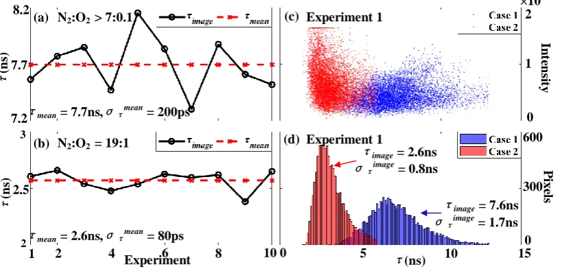
The variable, τimage, in Figs. 6(a) and 6(c) means the average lifetime for the whole excited area. Figures. 7(a) and 7(b) show τimage for ten repeated experiments for Cases 1 and 2, respectively. For Case 1, τimage is calculated by using Gating Scheme 1, the average τimage is τmean = 7.7ns and the standard deviation among these experiments is

στmean_{= 200ps as shown in Fig. 7(a). For Case 2, τimage is calculated by using Gating}

Scheme 2, τmean = 2.6ns and στmean= 80ps (but when we used Gating Scheme 1 for this, we obtained στmean _{= 150ps). It is convincing that the accuracy of the lifetime}

measurements is improved in the short lifetime range using TFI-TGFLI rather than

lifetimes. To use ORLD properly, it is necessary to have better understanding about the

lifetime distribution beforehand. The scatter plots, τ in the estimated lifetime images Figs. 6(a) and 6(c) vs the intensity in the corresponding intensity images Figs. 5(b) and 5(e), and the lifetime histograms for Experiment 1 are shown in Figs. 7(c) and 7(d), respectively. For Case 1 (blue), τimage = 7.6ns and the standard deviation for all the pixels in the lifetime image is στimage= 1.7ns. For Case 2 (red), τimage = 2.6ns and στimage= 0.8ns. As the gain of the ICCDs used in Case 1 is bigger than that used in Case 2, the largest intensity in Case 1 is larger than that in Case 2. The scatter plot for Case 1 contains 123 saturated pixels (peaked at 214_{-1), and they are contributed by the saturated 14-bit A/D}

converter. The statistical results are, however, not influenced. We can tune the gain in

the future to avoid saturated pixels.

1 2 4 _Experiment6 8 10

τimage = 2.6ns

στimage = 0.8ns

τimage = 7.6ns

στimage = 1.7ns

N2:O2 > 7:0.1

τmean = 7.7ns,

τmean = 2.6ns,

0 5 _τ 10 15

(ns) Experiment 1

Experiment 1 (d)

(c) (a)

N2:O2 = 19:1

(b)

0 2

1

In

te

n

sit

y

×104

0 600

300

P

ixe

ls

2

2.5

3

7.2 7.7 8.2

τ

(n

s)

τ

(n

s)

στmean = 200ps

στmean = 80ps

Fig. 7. Lifetime curves for (a) N2:O2 > 7:0.1 and for (b)N2:O2 = 19:1 among ten

repeated experiments. (c) Scatter plots and (d) lifetime histograms for Case 1 (blue)

and Case 2 (red) for Experiment 1.

(N2:O2 = 19:1), respectively. The A/D converter of the ICCD in the streak camera is

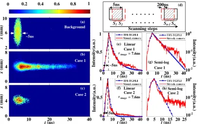
16-bit, and the actual peak intensities for Figs. 8(b) and 8(c) are 5400 and 2000, respectively. By integrating the images in Figs. 8(b) and 8(c) over the x axis, we obtained 1D normalized intensity curves (red lines) for Cases 1 and 2, as shown in Figs. 8(e) and 8(f). The blue open circle lines represent the results of TFI-TGFLI. Figs. 8(g) and 8(h) show the semi-log intensity curves for Cases 1 and 2. As the direction of the gas jet is parallel to the slit of the streak camera, the width of the slit is wide and a UV lens was used to gather the signal to the streak camera, the fluorescence from the total excitation region was collected by the streak camera. The temporal resolution is, however, deteriorated such that the signal detected in each scanning step has a duration

x (m m ) x (m m ) x (m m ) t (ns) (f) ~5ns ~5ns

S1S2 Sn-1Sn

Scanning steps

5ns 200ps (d)

0 0.2 0.4 0.6 0.8 1

0 4 8 0 4 8 2 6 10

0 10 20 30 40

Case 1 (a) Background (b) Case 2 (c) t (ns)

0 10 20 30 40

t (ns)

0 10 20 30 40

t (ns)

0 10 20 30 40

t (ns)

0 5 10 15 20 25

In te n sit y( a.u .) 10-2 10-1 100 In te n sit y( a.u .) 0 0.5 1 10-1 100 Case 2

τimage = 7.6ns

Linear (e)

Case 1

τimage = 7.6ns

Linear (g) Case 1 Semi-log (h) Case 2 Semi-log ~5ns 10-2 In te n si ty( a.u .) 0 0.5 1 In te n si ty( a.u .)

Fig. 8. (a) Background image without scanning, and the 1D lifetime images for (b) Case 1 and (c) Case 2 captured by the streak camera. (d) Schematic diagram

representing the scanning of the streak camera. Linear intensity curves for (e) Case 1 and (f) Case 2 obtained by integrating the 1D lifetime images (b) and (c) over the x

axis (red solid lines). The blue open circle lines represent the calculated results obtained by TFI-TGFLI. Semi-log intensity curves for (g) Case 1 and (h) Case 2.

5. Conclusion

We proposed a new rapid lifetime determination scheme on a multi-channel framing camera to achieve single-shot fluorescence lifetime imaging based on three images, and we coined it as TFI-TGFLI. The method combines the advantages of PLIF, time-gated FLI, and a multi-channel framing camera to perform single-shot acquisition. The

proposed TFI-TGFLI has a wide lifetime measurement range, 0.6 ~ 13ns, under the figure of merit Fi < 6, (i = τ, A). The lifetime images of the toluene seeded in gas mixtures of nitrogen and oxygen with different ratios were measured. Under N2:O2 >

7:0.1 (N2 = 7L/min; O2 < 0.1L/min) and N2:O2 = 19:1 (N2 = 19L/min; O2 = 1L/min)

respectively. They are consistent with the results obtained by the streak camera. A

further analysis on the relative concentrations of the quenchers and the fluorescent species shows a good agreement with the experimental settings. We believe that TFI-TGFLI can be an effective tool for complex flow diagnosis.

References

1. S. D. Hammack, C. D. Carter, J. R. Gord, and T. Lee, “Nitric-oxide planar laser-induced fluorescence at 10 kHz in a seeded flow, a plasma discharge, and a flame,”

Appl. Opt. 51(36), 8817–8824 (2012).

2. M. P. Lee, P. H. Paul, and R. K. Hanson, “Quantitative imaging of temperature fields

in air using planar laser-induced fluorescence of O2,” Opt. Lett. 12(2), 75–77 (1987).

3. Z. K. Wang, P. Stamatoglou, Z. M. Li, M. Alden, and M. Richter “Ultra-high-speed PLIF imaging for simultaneous visualization of multiple species in turbulent flames,”

Opt. Express 25(24), 30214–30228 (2017).

4. A. Ehn, J. J. Zhu, X. S. Li, and J. Kiefer, “Advanced laser-based techniques for gas-phase diagnostics in combustion and aerospace engineering,” Appl. Spectrosc. 71(5),

1–26 (2017).

5. C. Brackmann, J. Bood, J. D. Naucler, A. A. Konnov, and M. Alden, “Quantitative

picosecond laser-induced fluorescence measurements of nitric oxide in flames,” Proc.

Combust. Inst. 36, 4541–4548 (2016).

6. B. Zhou, C. Brackmann, Q. Li, Z. K. Wang, P. Petersson, Z. S. Li, M. Ald ´ en, and X. S. Bai, “Distributed reactions in highly turbulent premixed methane/air flames. Part

I. Flame structure characterization,” Combust. Flame 162, 2937–2953 (2015).

7. J. Philip, and K. Carlsson, “Theoretical investigation of the signal-to noise ratio in fluorescence lifetime imaging,” J. Opt. Soc. Am. A 20(2), 368–379 (2003).

8. H. C. Gerritsen, A. V. Agronskaia, A. N. Bader, and A. Esposito, “Time domain FLIM: Theory, instrumentation, and data analysis” in Laboratory Techniques in

Biochemistry and Molecular Biology, T. W. J. Gadella, ed. (Elsevier, 2009), pp. 95– 132.

(Springer, 2005).

10. G. O. Fruhwirth, S. A. Beg, R. Cook, T. Watson, T. Ng, and F. Festy, “Fluorescence lifetime endoscopy using TCSPC for the measurement of FRET in live cells,” Opt.

Express 18(11), 11148–11158 (2010).

11. S. Isbaner, N. Karedla, D. Ruhlandt, S. C. Stein, A. Chizhik, I. Gregor, and J. Enderlein, “Dead-time correction of fluorescence lifetime measurements and

fluorescence lifetime imaging,” Opt. Express 24(9), 9429–9445 (2016).

12. J. McGinty, J. R. Isidro, I. Munro, C. B. Talbot, P. A. Kellett, J. D. Hares, C. Dunsby, M. A. A. Neil, and P. M. W. French, “Signal-to-noise characterization of time-gated

intensifiers used for wide-field time-domain FLIM,” J. Phys. D: Appl. Phys. 42, 135103 (2009).

13. X. F. Wang, T. Uchida, D. M. Coleman, and S. Minami, “A two-dimensional fluorescence lifetime imaging system using a gated image intensifier,” Appl. Spectrosc.

45(3), 360–366 (1991).

14. D. D. U. Li, S. Ameer-Beg, J. Arlt, D. Tyndall, R. Walker, D. R. Matthews, V. Visitkul, J. Richardson, and R. K. Henderson, “Time-domain fluorescence lifetime

imaging techniques suitable for solid-state imaging sensor arrays,” Sensors 12(5), 5650-5669 (2012).

15. E. Gratton, M. Limkeman, J. R. Lakowicz, B. P. Maliwal, H. Cherek, and G. Laczko, “Resolution of mixtures of fluorophores using variable-frequency phase and

modulation data,” Biophys. J. 46, 479-486 (1984).

16. M. A. Digman, V. R. Caiolfa, M. Zamai, and E. Gratton, “The phasor approach to fluorescence lifetime imaging analysis,” Biophys. J. 94, L14-L16 (2008).

17. M. Jonsson, A. Ehn, M. Christensen, M. Alden, and J. Bood, “Simultaneous one-dimensional fluorescence lifetime measurements of OH and CO in premixed flames,”

Appl. Phys. B Lasers Opt. 115, 35–43 (2014).

18. A. Omrane, F. Ossler, and M. Aldén, “Two-dimensional surface temperature

measurements of burning materials,” Proc. Combust. Inst. 29(2), 2653-2659 (2002).

19. A. Ehn, O. Johansson, J. Bood, A. Arvidsson, B. Li, and M. Alden, “Fluorescence

20. S. P. Chan, Z. J. fuller, J. N. Demas, and B. A. DeGraff, “Optimized gating scheme for rapid lifetime imaging,” Anal. Chem. 73(18), 4486–4490 (2001).

21. A. Ehn, O. Johansson, A. Arvidsson, M. Alden, and J. Bood, “Single-laser shot fluorescence lifetime imaging on the nanosecond timescale using a Daul Image and Modeling Evaluation algorithm,” Opt. Express 20(3), 3044–3056 (2012).

22. A. Ehn, M. Jonsson, O. Johansson, M. Alden, and J. Bood, “Quantitative oxygen concentration imaging in toluene atmospheres using Dual Imaging with Modeling Evaluation,” Exp. Fluids 54, 1433 (2013).

23. R. K. Hanson, R. M. Spearrin, and C. S. Goldenstein, Spectroscopy and Optical Diagnostics for Gases, (Springer, 2016), Chap. 11.

24. D. U. Li, E. Bonnist, D. Renshaw, and R. Henderson, “On-chip, time-correlated, fluorescence lifetime extraction algorithms and error analysis,” J. Opt. Soc. A 25(5),

1190–1198 (2008).

25. A. Draaijer, R. Sanders, and H. C. Gerritsen, “Fluorescence lifetime imaging, a new tool in confocal microscopy,” in Handbook of Biological Confocal Microscopy, J. B.

Pawley, ed. (Plenum, 1995), pp. 491–505.

26. S. Faust, T. Dreier, and C. Schulz, “Temperature and bath gas composition dependence of effective fluorescence lifetimes of toluene excited at 266 nm,” Chem.