Generalised ambiguity function for MIMO radar systems

(1)

Generalised Ambiguity Function for MIMO Radar

Systems

Christos V. Ilioudis,

Member, IEEE,

Carmine Clemente,

Member, IEEE,

Ian Proudler,and John Soraghan

Member, IEEE,

Abstract—In this work a generalised signal model is presented to accommodate both narrowband and wideband signals in a multi-input multi-output (MIMO) sensor system scenarios. The derived model is then used to define a MIMO ambiguity function (AF) based on the Kullback-Leibler divergence (KLD). Moreover, the proposed formulation is parametrised using the signal and channel correlation matrices to account for different waveform and sensor placement designs, thereby allowing a flexible modelling approach. A comparison between the proposed definition and the more conventional approach of summing the squared matched filter outputs is presented for different sensors and waveforms configurations.

Index Terms—Multiple-Input and Multiple-Output Ambigu-ity Function (MIMO-AF), Multiple-Input and Multiple-Output Radar System, Kullback-Leibler divergence (KLD).

I. INTRODUCTION

M

IMO (multiple-input multiple-output) radar systems have attracted the interest of the research community due to their ability to significantly improve their performance compared to the traditional monostatic and multistatic systems. Although MIMO can be generally viewed as a type of multi-static radar, in this work the characteristic difference between the two arises from the distinction of waveforms attributed to each transmitter and the joint processing that MIMO is predicated on [1].

Following the aforementioned definition, the MIMO radar systems can be mainly classified into two extreme configura-tions, being the co-located and widely distributed, depending on the spatial allocation of their antennas. The various ad-vantages of both co-located and distributed arrangements are discussed in [2] and [3] respectively. Additionally, as shown in [2] and [4] the systems can also be categorised based on the coherency of their operating waveforms with the special cases of fully orthogonal and coherent signals. Moreover the importance of the target model in MIMO systems was discussed in [1] and [5] where it was described how the covariance of the transmitter-target-receiver channel matrix is associated with the geometry of the system and the dimension of the target.

Modern radar systems are required to operate with high accuracy for their intended application. It is therefore very important to have prior knowledge of the system’s expected

C. V. Ilioudis, C. Clemente, I. Proudler and J. Soraghan are with the Centre for Signal and Image Processing, Department of Elec-tronic and Electrical Engineering, University of Strathclyde, Glasgow G1 1XW, U.K. (e-mail: [email protected], [email protected], [email protected], [email protected]).

Manuscript received Oct 26 , 2018.

performance from the design stage. One of the most used tools in radar engineering is the ambiguity function (AF). Originally introduced by Woodward [6], the AF is a graphical represen-tation of the received signal’s response when a matched filter is applied for different delays and Doppler shifts. Using the AF it is therefore easy to extract valuable information such as the ambiguities and resolution expected for a particular configuration.

The traditional AF applies on monostatic narrowband sys-tems. However, ever since it was firstly introduced various interpretations were adapted to suit different applications of interest. Namely a number of wideband AFs have been inves-tigated in [7]–[9] while in [10] an AF parametrised by azimuth, elevation, range and Doppler was introduced.

In the later years, due to the promising tendency of radar technology to extend into multi-sensor/multi-platform con-figurations, various formulations of AFs for MIMO systems have been proposed [2], [4], [5], [11], [12]. In [4] and [11] the optimum detector concept is used and the MIMO AF is obtained by summing the matched filtered result from each receiver. In [13] and [14], a MIMO AF definition similar to the one proposed in [4], which considers however arbitrary transmit power allocation, was proposed in order to examine MIMO radar with correlated waveforms. The performance improvement of the proper waveform correlation matrix de-sign was also illustrated though a comparison with the AF metric defined in [15], where spatially diverse waveforms are proposed. Lastly, the authors in [16] used the matched filter definition to derive an AF and its properties, for a special case of MIMO radar, called phased-MIMO radar, in which waveform diversity was employed to divide an array into phased subarrays.

Under the similar concept of matched filter summation, a MIMO AF based on a general ultrawideband signal model is derived in [17]. Here, the authors also propose a factorisation of three MIMO AF parameters, the transmitted signal, system topology, and relative motions, while an analysis is presented focusing on how each of these parameters affect the perfor-mance of the system without calculating the entire MIMO AF. Furthermore, in [18] a MIMO AF based on the squared-sum of all matched filter responses was derived as an analytic tool for designing orthogonal ultrawideband impulse waveforms.

(2)

between 0 and1. Moreover, the authors derive a formulation composed of the transmitted signals’ expected and actual matched filter outputs while a comparison of the proposed MIMO AF was also carried out under different transmitted waveforms scenarios. In [12] a log-likelihood based MIMO AF was derived based on bistatic MIMO radar systems. A similar log-likelihood based MIMO AF definition, was also applied on a widely distributed MIMO system signal model in [5]. Additionally, an optimisation of the MIMO AF [5] through waveform design is presented in [20].

Lastly, a MIMO AF based on the KLD and a distributed MIMO radar signal model is derived in [21]. Although the approach of formulating the MIMO AF in [21] and [5] are very similar, the authors in [21] derive a formulation of the inverse covariance matrix of the expected signal. This specific approach reduces computation complexity and derives a bounded function with lower and upper limits 0 and 1 respectively, similar to [19].

In this work a generalised signal model is presented to accommodate both narrowband and wideband signals in a MIMO sensor system scenarios. The derived model is then used to define a MIMO AF based on the KLD similar to the one presented in [21], which however covers only narrowband signals in widely distributed MIMO systems. Moreover, the proposed formulation is parametrised by the signal and the channel correlation matrices. This allows for more flexible modelling compared to the approach in [2], where the channel correlation matrix needs to be factorised. The contribution of the presented work is summarised as follows:

• The paper provides a channel correlation matrix based on a generalised, wideband signal model and proposes an approximation for distributed and co-located configu-rations;

• The paper defines a generalised MIMO AF and examine its behaviour for different signals and sensors configura-tions;

• The paper compares the proposed MIMO AF with the summation of the matched filter outputs from all transmitter-receiver pairs in simulated scenarios.

The remainder of the paper is organised as follows. Section II introduces the MIMO radar framework used in this analysis. A formulation of the channel correlation matrix is presented in Section III. The proposed MIMO AF is derived in Section IV while illustrations of its behaviour under various configura-tions is shown in Section V. Later, in Section VI a comparison between the proposed definition and the conventional approach of summing the squared matched filter outputs is held in various simulated scenarios. Finally, Section VII summarises the outcomes of this work.

Comments on notation: Vectors and matrices are denoted by bold letters, e.g. `. The transpose and conjugate transpose operators are denoted by (·)T _and _(·)† _{respectively. The} Euclidean distance operation is denoted by | · |, δ(·)denotes the Dirac delta function, E{·} denotes the expected value, and j=√−1. Moreover, I` denotes a `×` identity matrix,

1` is a `×` square matrix populated by ones, diag(·) a

diagonal or block diagonal matrix, and “⊗” is the Kronecker product operation. Finally, for convenience and without loss of generality, in the rest of the paper a 2-D plane is assumed instead of a 3-D space, with the general format of coordinates and velocity being expressed asx= [x, y]T _and_u_{= [}_u

x, uy]T respectively.

II. SIGNALMODEL

Let us consider a MIMO radar system configuration con-sisting of NT transmitters and NR receivers, with all their antennas having an isotropic radiation pattern. The location and velocity of the i-th transmitter and the j-th receiver are denoted in the Cartesian plane by the column vectorsxi,T and

ui,T fori= 1, . . . , NT, andxj,Randuj,Rforj= 1, . . . , NR respectively. Moreover, assume an extended target within the surveillance area consisted by a finite number NQ of independent isotropic scatterers with location and velocity defined respectively byxq,Qanduq,Qforq= 1, . . . , NQ. The reflectivity of the scatterer is modelled by an independent and identically distributed (i.i.d) complex random variableζq with zero mean and variance E{|ζq|2}=σ20/NQ, where σ02 is the

average radar cross section (RCS) of the target. Additionally the target is assumed to follow the classic Swerling I model, while its RCS centre of gravity is located at x0,Q and its velocity isu0,Q.

The propagation of a signal from a transmitter to a receiver consists of three sequential steps: 1) the propagation from a transmitter to the scatterers of the target, 2) the reflection from the scatterers and 3) the propagation from the target to a receiver. Considering a stationary system, the delay of a signal emitted byi-th transmitter, reflected by theq-th scatterers and received byj-th receiver can be written as:

τ_j,i(q)= |D

(q) i,T|+|D

(q) j,R|

c (1)

where D(_i,q_T) = xq,Q−xi,T and D(j,qR) = xq,Q −xj,R are the distance vectors from the q-th scatterer of the target to thei-th transmitter andj-th receiver respectively, andcis the speed of light. If the relative motion within the transmitter-target-receiver system is also taken into account, the delay of the signal will vary in time and can be described in a Taylor seriesτ˜_j,i(q)(t)around a certain time referenceτ_j,i(q):

˜

τ_j,i(q)(t) =τ_j,i(q)+ (t−τ_j,i(q))d dtτ˜

(q) j,i(τ

(q) j,i)

+(t−τ

(q) j,i)2

2! d2 dt2τ˜

(q) j,i(τ

(q)

j,i) +. . . (2)

wheredn_/_d_tn_{denotes the}_n_{-th order derivative with respect to} time. Under the assumption that the total range varies slowly with time over the coherent processing interval, the higher order components can be neglected [22] and the delay in (2) can be approximated by:

˜

τ_j,i(q)(t)≈τ_j,i(q)+ (t−τ_j,i(q))d dtτ˜

(q) j,i(τ

(q)

(3)

Furthermore, the first-order derivative can be calculated as:

d dtτ˜

(q) j,i(τ

(q)

j,i) = (U (q) i,T)

T D (q) i,T |D(_i,q_T)|+ (U

(q) j,R)

T D (q) j,R |D(_j,q_R)|

!

/c

(4) where U(_i,q_T) = uq,Q−ui,T and U

(q)

j,R = uq,Q−ui,R are the relative velocity vectors between the q-th scatterer and the i-th transmitter and j-th receiver respectively at the time referenceτ_j,i(q). To simplify, it is assumed that all the scatterers have the same velocity as the gravity centre of the target, i.e.

d dt˜τ

(q) j,i(τ

(q) j,i)≈

d

dtτ˜j,i(τj,i)

=

(Ui,T)T

Di,T |Di,T|

+ (Uj,R)T

Dj,R |Dj,R|

/c

(5)

where Ui,T = u0,Q −ui,T and Uj,R = u0,Q − ui,R are the relative velocity vectors and, Di,T = x0,Q−xi,T and Dj,R=x0,Q−xj,R are the distance vectors between the centre of gravity of the target and the i-th transmit-ter and j-th receiver respectively at the time reference

τj,i= (|Di,T|+|Dj,R|)/c. Accounting for the two-way radar equation and for unit RCS, the energy propagated fromi -th transmitter,q-th scatterer andj-th receiver path is calculated as:

E_j,i(q)≈Ej,i=

ˆ

Ei,T Gi,T Gj,R λ2 (4π)3_|_D

i,T|2|Dj,R|2Lj,i

(6)

where Eˆi,T and Gi,T are the energy and gain at the i-th transmitter respectively,Gj,R is the gain at thej-th receiver,

λis the wavelength of the carrier, andLj,idenotes other non free-space losses in the i-th transmitter j-th receiver path. It should be noted that the approximation in (6) holds by taking the reasonable assumption that the distance between the different scatterers and the RCS centre of gravity of the target is significantly smaller than its distance from each transmitter and receiver, and hence |D(_i,q_T)|2_|_D(q)

j,R|2≈ |Di,T|2|Dj,R|2. The received signal at the j-th receiver due to the i-th transmitter can be therefore expressed as:

rj,i(t) =

p Ej,i

NQ X

q=1 ζqgi

t−τ˜_j,i(q)(t)+nj(t) (7)

wheregi(t)is the normalised signal,R_T|gi(t)|2dt= 1, emitted form the i-th transmitter, and nj(t) is a complex additive Gaussian noise with distribution CN(0, σ2n), whereσ2n is the variance of the noise. Additionally, by substituting (3) in (7) the received signal can be expressed as:

rj,i(t) =

p Ej,i

NQ X

q=1 ζqgi

αj,i(t−τ (q) j,i)

+nj(t) (8)

whereαj,iis the time scaling factor defined as:

αj,i= 1−

d

dtτ˜j,i(τj,i) (9)

Following the analytic signal representation, the signal gi(t) can be expressed as:

gi(t) =si(t)ej2πfct (10)

wheresi(t)is the complex envelope of the signal from thei-th transmitter andfcis the carrier frequency. By substituting (10) in (8) and after removing the carrier the received signal can be expressed as:

rj,i(t) =

p Ej,i

NQ X

q=1 ζqeφ

(q) j,i_s_i

αj,i(t−τ (q) j,i)

ejωj,it₊_n

j(t)

(11)

where ωj,i = 2πfc(aj,i −1) and φ (q)

j,i = −j2πfcaj,iτ (q) j,i account respectively for the angular frequency and phase shifts applied to the signal due to the relative motion and delay in the

i-th transmitter,q-th scatter,j-th receiver system. Furthermore, under the assumption that the resolution of the baseband signalssi(t) is not high enough to distinguish the individual scatterers it can be shown that:

si(t−τ (q)

j,i)≈si(t−τj,i) (12) Additionally, for simplicity two intermediate variables are introduced:

h(_j,iq)(θ) =pEj,iζqeφ

(q)

j,i ₍₁₃₎

yj,i(t,θ) =si(αj,i(t−τj,i))ejωj,it (14)

wereθ= [x0,u0]T and therefore (11) can be expressed as:

rj,i(t,θ) = NQ X

q=1

h(_j,iq)(θ)yj,i(t,θ) +nj(t) (15)

Since the received signal is sampled at the receiver before being processed, it is more practical to define the total received signal by using aM×1column vector, whereMis the number of captured samples by each receiver. The total received signal can therefore be expressed by a NRM ×1 block matrix described as:

r(θ) =Y(θ)H(θ) +n (16)

whereY(θ)is defined as theNRM×NTNRblock diagonal matrix accounting for the changes in complex envelope and frequency of the signal for each transmitter-receiver pair,H(θ) is defined as the NRNT ×1 block matrix accounting for the phase and amplitude distortion of the signal, and n is a

NRM×1block diagonal matrix populated by noise. Equation (16) is derived in Appendix A.

From (16) and Appendix A we associateY(θ),H(θ)andn

as the discretised values of the continuous variablesyj,i(t,θ),

h(_j,iq)(θ) and nj(t) respectively for each transmitter-receiver combination. Moreover, it is useful to further factorisedH(θ) as:

H(θ) =pE(θ)K(θ)Z (17)

whereE(θ)is aNRNT×NTNRdiagonal matrix associated with the propagation lossesEj,i,K(θ)is aNRNT ×NQNR

block diagonal matrix accounting for the phase termeφ(j,iq)_{, and}

(4)

complex reflectivity ζq. It is worth noting that as the same values of reflectivity ζq will be experienced by all receivers,

Zis composed byNR duplicates of aNQ×1column vector containing the complex reflectivity of each scatterer.

It should be mentioned at this point that no specific assump-tions have been made regarding the geometry of the system. In the next section the behaviour of the phase channel matrix

H(θ)in different spatial configurations will be discussed.

III. CHANNELCORRELATIONMATRIX

As was shown in the previous section the received signal is composed of its complex envelope and frequency matrix

Y(θ)and the channel matrix H(θ)accounting for phase and amplitude shifts. In this section the covariance matrix ofH(θ) will be modelled for arbitrary spatial system configurations. Additionally, the two extremes of co-located and widely distributed cases will be examined separately. The proposed formulation was introduced and presented thoroughly in [23]. In this work, this conceptual framework is extended taking into account the relative velocity between target and sensors. Following the signal model in Section II, the covariance matrix C(θ) of the channel matrix H(θ) can be calculated as:

C(θ) =E{H(θ)H(θ)†}

=pE(θ)K(θ)EnZe o

K(θ)†pE(θ) (18)

where under the assumption that the complex reflectivity of the scatterers is uncorrelated i.e. E

ζq†ζq0 =δ(q−q0)|ζ_q|2,

the NRNQ×NQNR matrixZe=ZZ† is given as:

e

Z=1NR⊗diag(|ζ1| 2_,

|ζ2|2, ...,|ζNQ| 2₎

(19)

From (18) and (19) it can be easily shown that each element of C(θ)could be written as follows:

C(θ)(i,j)(i0_,j0₎=pE_i,jE_i0_,j0

NQ X

q=1

|ζq|2e φ(_j,iq)−φ(q)

j0,i0 ₍₂₀₎

where the subscript index (i, j)(i0, j0) imply the element in

C(θ) referring to the correlation between the i-th, j-th and

i0-th,j0-th transmitter-receiver channels, or more precisely, the element of which the row and column are given as

i+NT(j−1) andi0+NT(j0−1)respectively.

To get a better understanding of the how the summation in (20) behaves, first let us express the delayτ_j,i(q) as a function of sensors and scatterers coordinates [23]:

τ_i,(q_T)≈τi,T + ˜

xT_q,QDi,T

c|Di,T|

(21)

where x˜q,Q = [˜xq,Q,y˜q,Q]T, with x˜q,Q=xq,Q−x0,Q and

˜

yq,Q=yq,Q−y0,Qbeing the coordinates of theq-th scatterer when the target’s centre of gravity is considered the centre of axes. Following the same process for the delay from the

q-th scatterer to the j-th receiver the total phase can be approximated as:

φ(_j,iq)=φj,i+ ˜φ (q)

j,i (22)

whereφj,i=−j2πfcαj,iτj,i andφ˜ (q)

j,i is given as:

˜

φ(_j,iq)=−j2παj,i

˜

xT_q,_Q

_D

i,T |Di,T|

+ Dj,R |Dj,R|

/λ (23)

Using (22), the summation term in (20) can now be approxi-mated as:

NQ X

q=1

|ζq|2e

φ(_j,iq)−φ(q)

j0,i0 ₌_eφj,i−φj0,i0

NQ X

q=1

|ζq|2e ˜ φ(_j,iq)−φ˜(q)

j0,i0 ₍₂₄₎

As discussed in Section II, the target is assumed to be com-posed of a large number of NQscatterers. By definition, two scatterers cannot share the same location, i.e. xq,Q 6= xq0_,Q

forq6=q0, while a scatterer’s distance from the target’s centre of gravity in thex-axis andy-axis is bounded by the target’s dimensions in the respective axis, i.e.:

−∆x/2≤x˜q,Q≤∆x/2 (25)

−∆y/2≤y˜q,Q≤∆y/2 (26)

It is therefore reasonable to describe the reflectivity ζq as a function of target’s dimensions rather than the indexq:

ζq=Z(˜xq,Q,y˜q,Q) (27)

whereZ(x, y) denotes the complex reflectively of the target at the x∈[−∆x/2,∆x/2]and y ∈[−∆y/2,∆y/2]location point relative to its centre of gravityx0,Q.

Assuming that the scatterers’ location in the area occupied by the target is sampled from a uniform distribution, forNQ approaching infinity, Z(x, y) can be modelled as a complex random variable with zero mean and variance given by [23]:

E

|Z(x, y)|2 ₌ σ0

∆x∆y

(28)

By mapping the scatterer indexed reflectivity and phase terms, see |ζq|2 andφ˜

(q)

j,i, to their respective location indexed coun-terparts using (23) and (27), the weighted phases summation in (24) can be reformed as:

E

(NQ

X

q=1

|ζq|2e ˜ φ(_j,iq)−φ˜(q)

j0,i0

)

=

Z ∆x/2

−∆x/2

Z ∆y/2

−∆y/2 E

|Z(x, y)|2

×e−j2π[x,y]

αj,i

_D

i,T |D_i,_{T |}+

D_j,R |D_j,_{R |}

/λ

×ej2π[x,y]

α_j0_,i0

_D

i0,T |D_i0_,T|+

D_j0,R |D_j0_,R|

/λ

dydx

=σ₀2sinc π∆x

αj,i

_x

i−x0

|Di,T|

+xj−x0 |Dj,R|

−αj0_,i0

xi0−x₀

|Di0_,_T|

+xj0 −x0 |Dj0_,_R|

/λ !

×sinc π∆y

αj,i

_y

i−y0

|Di,T|

+ yj−y0 |Dj,R|

−αj0_,i0

_y

i0−y₀

|Di0_,_T|

+yj0−y0 |Dj0_,R|

/λ !

(5)

Transmitters Receivers

(a) Distributed

[image:5.612.336.539.55.186.2]

(b) Co-located

Figure 1. System geometry assuming (a) distributed and (b) co-located sensor allocation.

where Ω(θ)(i,j)(i0_,j0₎ denotes the elements of the NRNT ×NTNR channel correlation matrix Ω(θ). The relationship between the integral of complex exponentials and the sincfunction is given in Appendix B.

Using (29) a relationship between two arbitrary variables, namely the reflectively and position of a large number of scatterers, can be expressed in terms of meaningful properties of the target such as its dimensions. A more simplified expression of C(θ)can therefore be given as:

C(θ) =pE(θ)K0(θ)E {Ω(θ)}K0(θ)† p

E(θ) (30)

Here, K0(θ)is the NRNT ×NTNR diagonal matrix popu-lated by the steering vectors of each transmitter-receiver pair:

K0(θ) = diag(eφ1,1, eφ1,2, ...eφNR,NT) (31)

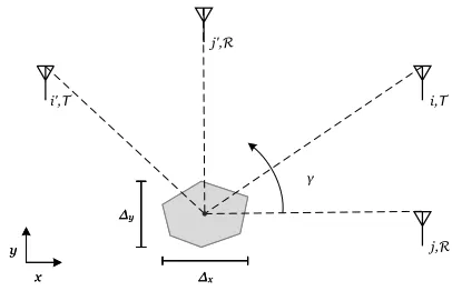
In the following, two different system geometries will be examined. Particularly the cases of fully distributed and co-located configurations will be discussed. A high level illustra-tion of the distributed geometry and co-located geometry are shown in Fig. 1a and Fig. 1b respectively.

A. Distributed System

The first spatial configuration considered is the widely distributed case. In this scenario the system’s sensors are assumed to be in such spatial orientation, so that the different transmitter-target-receiver paths can be considered uncorre-lated [23]. For a better understanding, in Fig. 1 the contribution of each transmitter-target path is illustrated by a different arrow color (hollow and filled) while the contribution from the target-receiver path is illustrated by different line (dashed and dotted). As can be seen for the distributed case, see Fig. 1a, each transmitter-receiver pair is characterised by a different arrow-line combination. In a distributed case the correlation matrix Ω(θ) can therefore be approximated by a diagonal matrix indicating that thei-th,j-th andi0-th, j0-th transmitter-receiver channels are uncorrelated. From (29) it can be seen

j,R j',R

i,T

Δy

Δx Δy

Δx

γ

x y

i',T

Figure 2. Example of two transmitter-receiver pairs(i, j)and(i0, j0)and a

target with dimensions∆x and∆y, with each sensor’s line of sight (dashed

line) having a different angleγwith the positive x-axis

that for the non-diagonal elements ofΩ(θ)to be approximated by0 at least one of the following conditions must hold:

αj,i

_x

i−x0

|Di,T|

+xj−x0 |Dj,R|

−αj0_,i0

_x

i0−x₀

|Di0_,_T|

+xj0−x0 |Dj0_,_R|

≥

λ

∆x (32)

αj,i

_y

i−y0

|Di,T|

+ yj−y0 |Dj,R|

−αj0_,i0

_y

i0−y₀

|Di0_,_T|

+ yj0−y0 |Dj0_,_R|

≥

λ

∆y (33)

The resulting conditions are similar to those presented in [1], scaled however by the time scaling factor and more importantly having dependency on the target’s position. Using (32) and (33), and assuming a sub-reference coordinate system with centre of axes the target’s centre of gravity andαj,i≈1 for all transmitter-receiver pairs, these conditions can also be expressed as:

cos(γi)−cos(γi0) + cos(γj)−cos(γj0)

≥

λ

∆x

(34)

sin(γi) −sin(γi0) + sin(γj) −sin(γj0)

≥

λ

∆y

(35)

where γ denotes the aspect angle, starting from the positive

x-axis, of which the respective node is facing the target. For a better understanding, in Fig. 2 an illustration of the described geometry is given. As it can be seen from the aforementioned conditions, to assume that a system is widely distributed a priori knowledge of the target’s expected position is required. If one of the conditions in (32) and (33) or (34) and (35) are satisfied, the elements of the matrix H(θ) can be assumed uncorrelated and thus its covariance matrixC(θ)can be expressed as:

C(θ) =pE(θ)K0(θ)INRNTK0(θ)

†p

[image:5.612.62.282.69.191.2]

(6)

B. Co-Located System

In a co-located configuration, it is assumed that the sensors can be divided into two groups, one composed of transmitter and one of receiver nodes. Furthermore, sensors in the same group are located in a very close proximity to each other compared to their distance from the target. This makes all the transmitter-target paths and all target-receiver paths to exhibit similar contributions respectively, see Fig. 1b.

Flowing this approach, the system’s sensors in a co-located case can be modelled into the transmitters’ and receivers’ clusters with centres of gravity atx0,T andx0,R respectively. It is therefore reasonable to assume that all the sensors in each cluster experience the same delay to and from the individual scatterers of the target. Moreover, it is assumed that all the sensors in each cluster experience similar velocity, u0,T for transmitters and u0,R for receivers respectively. Under these assumptions it is valid to use the same approximate time scaling factor for all the transmitter-receiver pairs:

αj,i≈α= 1−

(U0,T)T

D0,T |D0,T|

+ (U0,R)T

D0,R |D0,R|

/c

(37) where D0,T =x0,Q−x0,T and D0,R=x0,Q−x0,R are the distance vectors, and U0,T =u0,Q−u0,T and

U0,R=u0,Q−u0,R are the relative velocity vectors between the target’s centre of gravity and the transmitters’ and receivers’ centre of gravity respectively. Additionally, the total time delay in the i-th transmitter, target, j-th receiver path can be expressed as:

τi,j=τi,T +τj,R (38)

where τi,T = |D0,T|/c andτj,R =|D0,R|/c are the delays from the transmitter and the receiver to the gravity centre of the target respectively. From (37) and (38) it is derived that the observed phase φj,i can be decomposed as:

φi,j ≈φi,T +φj,R (39)

where φi,T = 2πfcατi,T andφj,R = 2πfcατj,R. Under this approximation it can seen that K0(θ) in (31) can be also

decomposed as:

K0(θ) =KT(θ)KR(θ) (40)

whereKT(θ)is theNRNT×NTNRdiagonal matrix defined as:

KT(θ) =INR⊗diag(e

φ1,T_{, e}φ2,T_{, ..., e}φN_T,T₎ ₍₄₁₎

andKR(θ)is theNRNT×NTNRdiagonal matrix given by:

KR(θ) = diag(eφ1,R, eφ2,R, ..., eφNR,R₎_⊗_I

NT (42)

The channel matrix H(θ)in (17) can therefore be expressed as:

H(θ) =pE(θ)KT(θ)KR(θ)Z (43)

From (29) it can be easily shown that if αj,i≈α and

xi,T ≈x0,T, the matrix Ω(θ) will be populated by ones scaled by the average RCS of the target. As a result, the ele-ments of the channel matrix H(θ)are completely correlated.

From (20) and (29) it can be deducted that to approxi-mate the co-located configuration, all the following conditions should be satisfied:

αj,i

_x

i−x0

|Di,T|

+xj−x0 |Dj,R|

−αj0_,i0

_x

i0−x₀

|Di0_,_T|

+xj0 −x0 |Dj0_,_R|

λ

∆x (44)

αj,i

yi−y0

|Di,T|

+ yj−y0 |Dj,R|

−αj0_,i0

_y

i0−y₀

|Di0_,_T|

+ yj0−y0 |Dj0_,R|

λ

∆y (45)

It is obvious that if αj,i≈α andxi,T ≈x0,T, the left part of the inequalities will always approximate close to 0 and therefore the co-located system can be considered independent of the position of the target.

IV. AMBIGUITYFUNCTIONFORMULATION

In this section a definition of the AF based on the Kullback-Leibler divergence (KLD) and the signal model described in Section II is provided. At this point it should be noted that the notion of using the KLD to describe ambiguity in radar and sonar measurement was originally introduced in [19] for the mono-static system case, while a similar KLD based MIMO AF formulation was introduced in [21]. The following discussion is focused on introducing the main concept of the KLD and it’s application for a MIMO AF formulation. For a more extended discussion the reader is referenced to [19], [21] and [24].

A. Kullback-Leibler Divergence (KLD)

The Kullback-Leibler Divergence (KLD) is a measure of difference between two probability distributions % and µ

[25], [26]. Depending on the specific application, %typically represents the “true” distribution of data, observations, or a precisely calculated theoretical distribution, while µ usually represents a theory or model description, or approximation of

%. The mathematical representation of the KLD from µto %

is denoted as:

I(%, µ) =E%

ln%

µ

(46)

where E%{·} is expectation with respect to the probability distribution%. The KLD can be also used as a sort of distance between % and µ. While the KLD does not satisfy all the properties of a distance such as symmetry and triangular inequalities, it can be shown that [26]:

I(%, µ)_>0 and I(%, µ) = 0⇔%=µ (47)

(7)

parameters and model mismatches, making it more suitable for broader applications such as passive systems. In Section II, the total received signalr(θ)in (16) is described as the summation of products between i.i.d random variables inH(θ)multiplied by the deterministic signals inY(θ). Assuming a large number of scatterersNQ, and invoking the central limit theorem, each target has a Gaussian distribution. Then since the received signal can be expressed as a linear combination of independent Gaussian variables, seeH(θ)andnin (16), the received signal follows a Gaussian distributionr∼ CN(0,Rθ). Moreover, the

covariance matrixRθof the received signal can be calculated

as [21]:

Rθ=E{r(θ)r(θ)†}

=Y(θ)C(θ)Y(θ)†+σ_n2IM NR (48)

The KLD between two M NR sized normal probability mea-sures with zero mean and covariance matricesRθ0 andRθ is

[19]:

I(θ0:θ) =

1 2 tr

R−_θ1Rθ0 −M NR

−ln det

R−_θ1Rθ0

(49)

In this case the two normal probability measures are those described by the return signal occuring when the target is placed at the spatial/velocity location θ0 and the expected

locationθrespectively [21]. Using (48) and by applying linear algebra the KLD in (49) are written as [21]:

I(θ0:θ) =

1 2 −tr

Ψ(θ0,θ)† C(θ0)

σ2 n

Ψ(θ0,θ) C(θ)

σ2 n

×

Φ(θ)C(θ)

σ2 n

+INTNR

−1

+ tr

Φ(θ0)

C(θ0) σ2

n

−tr

(

Φ(θ)C(θ)

σ2 n

Φ(θ)C(θ)

σ2 n

+INTNR

−1)

+ ln

det

Φ(θ)C(θ)

σ2 n

+INTNR

−ln

det

Φ(θ0)

C(θ0) σ2

n

+INTNR

!

(50)

where, for simplicity the waveform correlation matricesΦ(θ) andΨ(θ1,θ2)are defined as:

Φ(θ) =Y(θ)†Y(θ) (51)

Ψ(θ1,θ2) =Y(θ1)†Y(θ2) (52)

Note the KLD in (50) is expressed in terms of auto-correlation, cross-correlation and channel covariance matrices.

B. MIMO Ambiguity Function

Applying a similar analysis to the one presented in [19] for a single-input single-output system (SISO), and taking into consideration that it is desired for the AF to take values between 0 and 1, the MIMO AF is defined as:

AMIMO(θ0,θ),1−

I(θ0:θ)

Iub(θ0)

(53)

where Iub(θ0) is the upper-bound of I(θ0 : θ). Examining

the different terms in (50) it can be easily shown that all the traces and logarithms will return positive values. Moreover, to maximise the I(θ0 : θ), the upper bound of each term can

be examined separately and then combined altogether. It is worth noting that since the terms in (50) are not intendant, treating them separately will not provide a tight upper bound, i.e.Iub(θ0)≥max

θ I(θ0:θ), but a more relaxed limit.

Considering the first term in (50) and assuming that there is at least oneθ for whichY(θ)†Y(θ0) = 0, it conveys that

the maximum value of this term is also zero. Example of such cases can be forθ in which the difference between the tested and actual Doppler shift is large enough so that theY(θ)and

Y(θ0)do not overlap in the frequency domain. Furthermore,

by using the eigenvalue decomposition of the matrix product

Φ(θ)C(θ)(see Appendix C) the maximum value of the third term in (50) is calculated from the following relation:

−tr

_Φ₍_θ₎_C₍_θ₎_/σ2

n

Φ(θ)C(θ)/σ2

n+INTNR

≤ − SNRθ SNRθ+ 1

(54)

whereSNRθ= tr{Φ(θ)C(θ)}/σ2ndenotes the totalexpected signal-to-noise ratio on the resolution bin θ. Here the term expected is used as the SNRθ is calculated using the

auto-correlation matrix of Y(θ) and not its cross correlation with Y(θ0). Using the same process (see Appendix C), the

maximum value of the fourth and fifth terms in (50) can be written as:

ln det

Φ(θ)C(θ)/σ_n2+INTNR ≤SNRθ (55)

−ln det

Φ(θ0)C(θ0)/σn2+INTNR ≤0 (56)

Using (54), (55) and (56) the upper bound of the KLD in (50) can be calculated as:

Iub(θ0) =

1 2

SNRθ0+ max

θ SNR

2

θ/(SNRθ+ 1)

(57)

Inspecting (57) it is observed that the KLD can get its maximum value at the resolution binθ, in which theSNRθ is

also maximum. This is expected as the ability to discriminate between the true and the approximated PDFs p(r|θ0) and p(r|θ)will be better forθin which the SNR is higher. A closer examination reveals that the termSNRθcan be expressed as:

SNRθ= NR X

j,j0

NT X

i,i0

ReΦ(θ)(i,j)(i0_,j0₎C(θ)₍_i,j₎₍_i0_,j0₎ (58)

were the double index in the summations indicates the unique pairs i.e. P

m,m0[·] =P_mP

m

m0₌₁[·]. It can be therefore

de-duced that the defined SNRθ value is highly dependant on

the geometry of the system through the channel correlation matrix C(θ), and the design of the operating waveforms thought the waveform correlation matrix Φ(θ). For example waveforms for which the cross-correlation has a negative real part assuming that the target is located θ, will have lower SNRθ in cases of positive channel correlation than if the

channels were uncorrelated.

Having defined an upper bound it can be guaranteed that (53) has a positive value. Additionally, from (47):

(8)

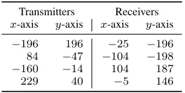
Table I

SENSORS’POSITION IN THE SURVEILLANCE AREA

x-axis y-axis x-axis y-axis

−196 196 −25 −196

84 −47 −104 −198

−160 −14 104 187

229 40 −5 146

The equality in (59) holds forθ = θ0→ I(θ0:θ) = 0and

therefore from (53) it can be shown that:

0≤ AMIMO(θ0,θ)≤1 ∀θ (60)

In previous work, it has been shown how under a constant SNRθ assumption, i.e. SNRθ = 1/σn2 the proposed KLD based AF definition in (53) can be reduced to a scaled sum of squared matched filter outputs [21]:

Acon,MIMO(θ0,θ) =

1

NTNR

trn|Ψ(θ0,θ)| 2o

(61)

Accounting for only one transmitter-receiver pair it can be eas-ily seen that (61) further reduces to the squared matched filter output of the expected and received signal which describes the conventional Woodward AF. A more detailed discussion on how the KDL definition relates to the Woodward AF for monostatic systems is held in [19]. Moreover, the relationship of the proposed MIMO AF with relative definitions is provided in [24].

V. EXAMPLES ANDILLUSTRATIONS

In this section a number of MIMO radar system config-urations will be examined to illustrate the behaviour of the proposed MIMO AF. To offer a broader understanding and keep the results generalised all the spatial values, values of speed, and bandwidths will be expressed as factors of the carrier wavelengths λ, carrier speed c, and as factor of the carrier frequencyfc respectively.

In Table I the locations of the sensors that will be used in this section is summarised. We define a (103_×₁₀3₎_λ2

surveillance area with the position of the sensors being chosen randomly in a (500×500)λ2 _{area centred at the centre of}

the scene. Moreover, the sensors’ velocities are considered 0 in both axes i.e. ui,T = [0,0]T, i = 1, . . . , NT and

uj,R = [0,0]T, i= 1, . . . , NR. In the following the above described system will be examined for different configurations.

A. Normalised Channel Correlation Matrix

In Section III a formulation of the covariance matrix was presented. To better illustrate how the channel correlation matrix varies through the different resolution bins, in Fig. 3a the normalised summation of the absolute value of non-diagonal elements in Ω(θ) is illustrated for a target with dimensions∆x= ∆y =λ. This quantity denotes the degree of correlation that the channels will have if the target is positioned

at the resolution binθ. Namely, the value for each resolution binθ is calculated as:

ˆ Ω(θ) =

NR X

j NT X

i NR X

j0

NT X

i0

δ δ(i−i0)δ(j−j0)

|Ω(θ)(j,i)(j0_,i0₎| NRNT(NRNT −1)

(62) From (62) it can be seen that for values ofΩ(ˆ θ)close to0the transmitter-receiver channels have a low degree of correlation and therefore the system can be better modelled by the widely distributed configuration Section III-A. On the contrary, for values close to1the channels have a high degree of correlation and the system can be better modelled by the co-located configuration, see Section III-B. As can be seen, areas closer to the centre of the scene where the target is surrounded by sensors from many directions are characterised by higher decorrelation between the channels. On the other hand, in more distant areas the channels are becoming more correlated as the sensors are facing the target from similar aspect angles. The same illustration for a target of dimensions ∆x = 1/2λ and

∆y = 2λ is presented in Fig. 3b. As can be seen, the area in which the channels are considered uncorrelated has been stretched parallel to the x-axis and squashed parallel to the

y-axis due to the different shape of the target.

B. Uncorrelated and Correlated Channels Performance

In this section the performance of the system will be assessed for different target placement and different operating waveforms. In all examples we consider a constant energy parameter for all resolution bins i.e.pE(θ) =INRNT.

1) Orthogonal waveforms: First let us consider a library of four orthogonal waveforms operating at each transmitter. The sequences used in the system are orthogonal frequency divi-sion multiplexed linear frequency modulated (OFDM-LFM) waveforms described as:

si(t) =ejπB(

1

Tt+i−1)t ₍₆₃₎

where T andB are the corresponding period and the band-width of the signal. All the variables of the system are summarised on Table II. In Fig. 4 the proposed MIMO AF is illustrated in logarithmic scale for a target with velocity

u0,Q = [0,0]T and centre of gravity is positioned at (a)

x0,Q= [0,0]T and (b)x0,Q= [−400λ,−400λ]T.

-500 -250 0 250 500 -500

-250 0 250 500

0.1 0.2 0.3 0.4 0.5 0.6 0.7 0.8

(a) Square target

-500 -250 0 250 500 -500

-250 0 250 500

0.1 0.2 0.3 0.4 0.5 0.6 0.7 0.8

[image:8.612.109.241.83.150.2]

(b) Parallelogram target

Figure 3. Normalized sum of non diagonal elements of the channel correlation

matrixΩfor target dimensions (a)∆x= ∆y=λand (b)∆x= 1/2λand

∆y= 2λ; transmitters and receivers are denoted by squares () and rhombi

(9)

-500 -250 0 250 500 -500

-250 0 250 500

-40 -35 -30 -25 -20 -15 -10 -5 0

(a) Uncorrelated

-500 -250 0 250 500 -500

-250 0 250 500

-40 -35 -30 -25 -20 -15 -10 -5 0

(b) Correlated

-100 -50 0 50 100

-30 -25 -20 -15 -10 -5 0

(c) Uncorrelated Zoomed

-500 -450 -400 -350 -300 -500

-450 -400 -350 -300

-30 -25 -20 -15 -10 -5 0

[image:9.612.52.298.63.299.2]

(d) Correlated Zoomed

Figure 4. MIMO AF with the target’s centre of gravity positioned in

(a)x0,Q= [0,0]T and (b)x0,Q = [−400,−400]T, and their respective

zoomed versions (c) and (d), when orthogonal waveforms are considered;

transmitters and receivers are denoted by squares () and rhombi (♦)

respectively.

Consulting Fig. 3 it can be seen that in the first target place-ment the transmitter-receiver channels can be characterised as uncorrelated while in the second case appear correlated. In Fig. 4c and Fig. 4d a zoomed version of the MIMO AF for these two cases is illustrated for regions close to the target’s position. In both cases, the MIMO AF is populated by 16 ellipsoid shaped ridges corresponding to each bistatic transmitter-target-receiver system, all of which intersect at the target’s location. On closer inspection it can be seen that in the uncorrelated channels case these ridges are added constructively to form a “smooth” representation with peak at the position of the target. In contrast, in the correlated case fluctuations are present due to the way the ridges from different correlated channels are added with each other. The ridges can be added constructively or destructively depending on the ridges being in-phase or off-phase and the correlation of the different channels being negative or positive.

The values of SNRθ for the examined scenario are

illus-trated in Fig. 5a. It is evident that theSNRθremains constant

in the entire area. This is expected as from (58) it can be seen that for orthogonal waveforms the sum will always be the total energy of the signals multiplied by the ratioNRNTσ02/σn2. To confirm that changing the system’s geometry will not impact the values of SNRθ, a different configuration is illustrated

in 5b. Here, the sensors are placed in a horizontal line with the transmitters and receivers being placed at the same point pairwise. As it can be seen, theSNRθremains constant in all

the examined area for both configurations.

2) Coherent Waveforms: In the second example the same system variables summarised in Table II will be assumed. In contrast to the previous section, here we assume that the

-500 -250 0 250 500 -500

-250 0 250 500

49 49.5 50 50.5 51

(a) Random

-500 -250 0 250 500 -500

-250 0 250 500

49 49.5 50 50.5 51

[image:9.612.347.528.661.745.2]

(b) Line

Figure 5. Values ofSNRθ in (a) random and (b) line sensor configuration,

when orthogonal waveforms are considered; transmitters and receivers are

denoted by squares () and rhombi (♦) respectively.

transmitters are using fully correlated waveforms given by:

si(t) =ejπ

B Tt

2

, i= 1, . . . ,4 (64)

To avoid confusion with channel correlation, fully correlated waveforms are referred to as coherent waveforms.

In Fig. 6 the MIMO AF of the system is illustrated for the two different positions of the target, in conjunction with a zoomed version of the MIMO AF for areas close to the target. Examining both figures it can be seen that in for coherent waveforms the number of ellipsoid ridges populating the MIMO AF is higher than when low cross-correlation waveforms are used. In fact, 64 ridges are formed as the different transmitters cannot be decorrelated at the receivers. A direct consequence of that is that the extra ridges will not fall on the target’s resolution bin if the resolution of the baseband signalsi, as determined by its bandwidth, is high enough. The impact of this phenomenon would be more apparent in the case of widely distributed systems and becomes less apparent as the system approaches the fully co-located case, where all the ridges will eventually overlap. Moreover, in Fig. 7 the values of SNRθ are illustrated across the surveillance area.

By comparing the results with the ones in Fig. 5 it can be seen that when the waveforms are non orthogonal, fluctuations in the SNRθ occur. From (58) it can be seen that those

fluctuations depend on the correlation between the channels and the degree of correlation that the waveforms will have at each resolution binθ. Comparing the random and line sensor configuration in 7a and 7b respectively it can be easily seen that by manipulating the system’s geometry it is possible to increase the SNRθ in areas of interest.

Table II

THEORETICALMIMO SYSTEMVARIABLES

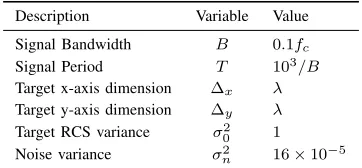
Description Variable Value

Signal Bandwidth B 0.1fc

Signal Period T 103_/B

Target x-axis dimension ∆x λ

Target y-axis dimension ∆y λ

Target RCS variance σ2

0 1

(10)

-500 -250 0 250 500 -500

-250 0 250 500

-40 -35 -30 -25 -20 -15 -10 -5 0

(a) Uncorrelated

-500 -250 0 250 500 -500

-250 0 250 500

-40 -35 -30 -25 -20 -15 -10 -5 0

(b) Correlated

-100 -50 0 50 100 -100

-50 0 50 100

-30 -25 -20 -15 -10 -5 0

(c) Uncorrelated Zoomed

-500 -450 -400 -350 -300 -500

-450 -400 -350 -300

-30 -25 -20 -15 -10 -5 0

[image:10.612.57.563.63.304.2]

(d) Correlated Zoomed

Figure 6. MIMO AF with the target’s centre of gravity positioned in

(a)x0,Q= [0,0]T and (b) x0,Q = [−400,−400]T and their respective

zoomed versions (c) and (d), when coherent waveforms are considered;

transmitters and receivers are denoted by squares () and rhombi (♦)

respectively.

-500 -250 0 250 500 -500

-250 0 250 500

47 48 49 50 51 52

(a) Random

-500 -250 0 250 500 -500

-250 0 250 500

47 48 49 50 51 52

(b) Line

Figure 7. Values ofSNRθin (a) random and (b) line sensor configuration,

when coherent waveforms are considered; transmitters and receivers are

denoted by squares () and rhombi (♦) respectively.

C. Target Velocity Mismatch

In this part, the behaviour of the proposed MIMO AF for a moving target will be examined for correlated and uncorrelated channels using orthogonal waveforms, see Section V-B. It should be noted that while the target has non zero velocity, a static target is assumed during the signal correlation process resulting in a velocity mismatch. In Fig. 8 the MIMO AF is illustrated for the two different channel configurations and two target speeds,u0,Q= [2×105λ/s,2×105λ/s]T and

u0,Q= [5×105λ/s,5×105λ/s]T. As can be seen for all cases, the ridges corresponding to the different transmitter-receiver pairs have been displaced and are no longer crossing at the real position, compared to Fig. 4. This phenomenon is expected and is related to the range-Doppler coupling that LFM waveforms exhibit.

Under closer inspection, it can be seen that for the uncor-related channels case, see Fig. 8a and Fig. 8c, the velocity of

-500 -250 0 250 500

-40 -35 -30 -25 -20 -15 -10 -5 0

(a) Uncorrelated

-500 -250 0 250 500

-40 -35 -30 -25 -20 -15 -10 -5 0

(b) Correlated

-500 -250 0 250 500

-40 -35 -30 -25 -20 -15 -10 -5 0

(c) Uncorrelated

-500 -250 0 250 500

-40 -35 -30 -25 -20 -15 -10 -5 0

[image:10.612.52.299.375.490.2]

(d) Correlated

Figure 8. MIMO AF with the target’s velocityu0,Q= [2×105,2×105]T

and centre of gravity positioned in (a) x0,Q= [0,0]T and (b)

x0,Q= [−400,−400]T, and for velocityu0,Q= [5×105,5×105]T for

the two different position in (c) and (d) respectively, when orthogonal waveforms are considered; transmitters and receivers are denoted by squares () and rhombi (♦) respectively.

the target causes the ridges to diverge in different directions as the relative velocity experienced by the bistatic pairs is also different. In contrast, when a correlated channel configuration is considered the ridges appear to converge in a relatively close area as the effective velocity by the bistatic pairs is also similar, see Fig. 8b and Fig. 8d. Moreover, comparing the two channel configurations for different velocities, it can be seen that the range-Doppler coupling related phenomenon becomes more apparent as the velocity increases. It is worth noting that as the velocity increases the ridges also appear to be more attenuated and wider. This is caused due to the mismatch between the received and reference signal, as well as the time stretching of the complex envelope due to the high relative velocity.

(11)

cuts, or sub-parts, of the MIMO AF for different target location and velocity parameters in a fixed waveforms and sensor locations configuration. In fact, in a system design scenario the optimal configuration of those fixed parameters is typically investigated. By observing the behaviour of the MIMO AF it can be seen that the system exhibits higher location-velocity coupling for targets at the corner of the surveillance area than for targets at its centre where sidelobes at different locations will appear.

VI. SIMULATIONS ANDCOMPARISON

In this section the performance of the proposed AF will be examined in a simulated MIMO radar scenario. It should be noted that the main difference compared to the previously presented analysis in Section V, is that here the received signal is extracted by simulating the returns of an extended target and not by using the mathematical model of the covariance matrix

Rθ0presented in (48). The impact of estimating the covariance

matrices and the required modifications that need to be made on the proposed MIMO AF will be discussed in the following paragraphs.

A. Modified AF and Correlation Matrix approximation

One of the main difficulties in applying the proposed AF definition using the KLD in (50) for simulated or real data, is that the received signal r0 cannot be decomposed into its

individual terms. As a result, the formulation in (50) has to be modified to accommodate the processing on the entire received signal r0 and not each its individual components

i.e. Y(θ0), C(θ0), and σn. For this reason the covariance matrix of the received signal, Rθ0, will be approximated by

its sample covariance matrix. Revisiting (49) and substituting

R0 =r0r†0, the trace and logarithmic terms of the KDL are

derived as follows:

tr

R−_θ1R0 =−tr

(

ˆ

Ψ(θ)†Ψˆ(θ)C(θ)

σ2 n

×

Φ(θ)C(θ)

σ2 n

+INTNR

−1)

+ 1

σ2 n

tr

(

r†₀r0 )

(65)

ln|R−_θ1R0|=−2M NRln(σn2)

−ln

det

Φ(θ)C(θ)

σ2 n

+INTNR

+ lndetnr0r†0 o

(66)

where Ψˆ(θ) is the 1 × NRNT row vector populated by the output of the received signal matched filtered for each transmitter-receiver pair i.e.:

ˆ

Ψ(θ) =r†₀Y(θ) (67)

Due to the high computational cost, the logarithmic terms in (66) will not be taken into account in the MIMO AF

computation. Therefore, assuming that det

R−_θ1R0 = 1

for every test resolution bin θ, the approximated KLD Iˆ is described as:

ˆ

I(θ0,θ) =

1 2 tr[R

−1

θ R0]−M NR (68)

Moreover the results are normalised so that the minimum and maximum values are always 0 and 1 respectively. The definition of the MIMO AF used in this scenario is given as:

ˆ

AMIMO(θ0,θ) = 1−

ˆ

I(θ0,θ)−min θ

ˆ I(θ0,θ)

max

θ

ˆ

I(θ0,θ)−min θ

ˆ I(θ0,θ)

(69)

The main reason of normalising the results is to provide an easier comparison between the theoretical and other proposed AFs.

A secondary matter in using the proposed definition on simulated or real data is that the definition of the channel correlation matrix in (29) and consequently the matrixC(θ0)

is based under the assumption that the target is composed of scatterers with a reflectivity modelled by i.d.d. complex random variables (see Section III). The main result of this assumption is thatE

ζ_q†ζq0 =δ(q−q0)|ζ_q|2, which is not true

if only an individual measurement ofζq is taken. To address this issue a coherent processing ofNP pulses is assumed. As a consequence, the received signalr0 has to be expressed by

a M ×NP matrix, each column of which contains the M samples of one coherent acquisition. Consequently the matrix

ˆ

Ψ(θ)will also change its size toNP×NRNT.

B. Simulated results

To evaluate the degree of similarity between the theoretical value of C(θ0) and the one expected from the simulation

ˆ

C(θ0), the Frobenius norm of their difference is calculated

and divided by the norm of the theoretical matrix, i.e. the approximation error is calculated as:

E = || ˆ

C(θ0)−C(θ0)||

||C(θ0)||

(70)

The sensors’ configuration is summarised in Table. I with the targets dimensions being ∆x = ∆y = λ, while two target locations x0 = [0,0]T and x0 = [−400,−400]T, are

used to approximate systems with uncorrelated and correlated channels respectively.

In Fig. 9 the resulting approximation error after a Monte Carlo of1000iterations is illustrated for a different number of coherent pulsesNP and a different number of scatterersNQ. Comparing the two configurations it can be seen that for un-correlated channels the approximation error is generally higher than for correlated. It is worth noting that while the Frobenius norm, ||Cˆ(θ0)−C(θ0)||, is in fact similar for both cases,

the C(θ0)for correlated channels has generally higher norm

(12)

0 50 100 150 200 0

0.2 0.4 0.6 0.8 1

(a) Uncorrelated

0 50 100 150 200

0 0.2 0.4 0.6 0.8 1

[image:12.612.313.563.64.175.2]

(b) Correlated

Figure 9. Normalised euclidean distance between the theoretical and simu-lated channel correlation matrix for an approximated (a) uncorresimu-lated and (b) correlated channel system.

Table III

SENSORS’POSITION IN SIMULATED SCENARIOS

Distributed Co-located

Transmitters Receivers Transceivers

x-axis y-axis x-axis y-axis x-axis y-axis

−1964 1961 −254 −1964 2500 0.1

840 −475 −1040 −1981 2500 0.5

−1606 −149 1045 1872 2500 −0.5

2291 406 −54 1463 2500 −0.1

cross-correlationζ_q†ζq0 will tend to zero. Moreover, comparing

[image:12.612.51.298.64.170.2]

the results for different values of NQ in the distributed case, Figure 9a shows that while higher number of scatterers will result to better approximation, the improvement saturated for

NQ > 100. On the other hand, for the co-located case it appears that the approximation behaves similarly for all the examined values of NQ. To evaluate the performance of the proposed AF, a 4×4 MIMO radar system with an extended target is simulated. The variables of the system are summarised in Table IV, while a coherent processing of NP = 50 pulses is used to generate the MIMO AF. For comparison, the more canonical approach of summing the square matched filter outputs is also employed, calculated as:

ˆ

Acan,MIMO= tr n

ˆ

Ψ(θ)†Ψˆ(θ)o (71)

The performance of the proposed and canonical MIMO AF is compared for a distributed and co-located system geometric configurations summarised in Table III. It should be noted that in all simulations, a5×5km2area is examined with the target located at x0,Q= [0,0].

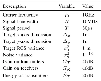
[image:12.612.72.279.247.327.2]

1) Distributed System: In the following paragraphs, the distributed configuration described in Table III is simulated to examine the behaviour of the proposed and canonical MIMO AF definition. First the system is explored using the orthogonal waveforms described in (63). In Fig. 10 the proposed and canonical MIMO AFs are illustrated. Comparing Fig. 10a and Fig. 10b, it is observed that both MIMO AFs have identical behaviour, being composed of 16 ridges corresponding to the NTNR = 16 individual transmitter-receiver pairs. The similarity in the results is expected and can be easily validated theoretically by replacing the correlation matrices Φ(θ) and

C(θ)with diagonals in (65).

-2500 -1250 0 1250 2500

-40 -35 -30 -25 -20 -15 -10 -5 0

(a) Proposed

-2500 -1250 0 1250 2500

-40 -35 -30 -25 -20 -15 -10 -5 0

(b) Canonical

Figure 10. Illustration of (a) proposed and (b) traditional MIMO AF in a distributed system configuration using orthogonal waveforms.

-2500 -1250 0 1250 2500

-40 -35 -30 -25 -20 -15 -10 -5 0

(a) Proposed

-2500 -1250 0 1250 2500

-40 -35 -30 -25 -20 -15 -10 -5 0

(b) Canonical

-700 -350 0 350 700

-30 -25 -20 -15 -10 -5 0

(c) Proposed Zoomed

-700 -350 0 350 700

-30 -25 -20 -15 -10 -5 0

(d) Canonical Zoomed

Figure 11. Illustration of (a) proposed and (b) traditional MIMO AF in

a distributed system configuration using coherent waveforms and zoomed

versions, (c) and (d) repectiely; the red line marks the−3dB contours of

the MIMO AFs, while the white line marks the contour where the proposed

MIMO AF is50%lower than the canonical.

Using the same geometry, the system was simulated using the coherent waveforms described in (64). In Fig. 11 the two MIMO AFs are illustrated. As it can be observed in Fig. 11a

Table IV

SIMULATEDMIMO SYSTEMVARIABLES

Description Variable Value

Carrier frequency f0 1GHz

Signal bandwidth B 10MHz

Signal period T 50µs

Target x-axis dimension ∆x 1m

Target y-axis dimension ∆y 1m

Target RCS variance σ20 1m

Noise variance σ2

n 1−13

Gain on transmitters GT 40dB

Gain on receivers GR 40dB

[image:12.612.356.520.615.747.2]

(13)

-2500 -1250 0 1250 2500 -2500

-1250 0 1250 2500

-40 -35 -30 -25 -20 -15 -10 -5 0

(a) Proposed

-2500 -1250 0 1250 2500

-40 -35 -30 -25 -20 -15 -10 -5 0

(b) Canonical

-700 -350 0 350 700 -700

-350 0 350 700

-50 -40 -30 -20 -10 0

(c) Proposed Zoomed

-700 -350 0 350 700 -700

-350 0 350 700

-50 -40 -30 -20 -10 0

Figure 12. Illustration of (a) proposed and (b) traditional MIMO AF in

a co-located system configuration using orthogonal waveforms and zoomed

versions, (a) and (b) repsectivelly; the red line marks the−3dB contours of

the MIMO AFs.

and Fig. 11b both MIMO AFs are composed of a larger number of ridges compared to when orthogonal waveforms are used. The actual number of ridges is N_T2NR = 64, as discussed in Section V-B. For a better examination, Fig. 11c and Fig. 11d offer zoomed illustrations of the MIMO AFs for an area close to the target. Moreover, a red line marks the −3dB contour of the two MIMO AFs, while in Fig. 11c the contour for which the proposed MIMO AF is 50%lower than the canonical is shown in white. Examining Fig. 11c, it is observed that the proposed MIMO AF has values over −3dB only in the main lobe to where the target is placed. In contrast, in Fig. 11d it is shown that the canonical MIMO AF exhibits a sidelobe of values higher than −3dB in a distant point from the target’s position. This is caused due to the way the canonical MIMO AF is constructed by adding all the resulting ridges constructively. Inspection of Fig. 11c shows that in those areas in which the different ridges are crossing, the value of the proposed MIMO AF is at least half of those in the canonical.

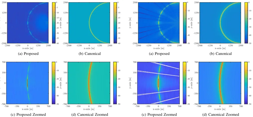
2) Co-located System: In this example scenario the co-located system configuration summarised in Table III is used. In Fig. 12 the resulting MIMO AFs are illustrated when the operating waveforms are orthogonal as given in (63). In both cases the MIMO AF is described by a circular ridge crossing the position of the target. In reality, as described in Section V-B, this ridge is composed of 16 secondary ridges corresponding to the individual transmitter-receiver pairs. To provide closer inspection, Fig. 12c and Fig. 12d illustrate the two different MIMO AFs only for the area close to the target, while a red line marks the −3dB contour. As it can be seen in Fig. 12c the proposed MIMO AF has a distinctive peak at the area surrounding the target while it reduces and

-2500 -1250 0 1250 2500

-50 -40 -30 -20 -10 0

(a) Proposed

-2500 -1250 0 1250 2500

-50 -40 -30 -20 -10 0

(b) Canonical

-700 -350 0 350 700 -700

-350 0 350 700

-50 -40 -30 -20 -10 0

(c) Proposed Zoomed

-700 -350 0 350 700 -700

-350 0 350 700

-50 -40 -30 -20 -10 0

Figure 13. Illustration of (a) proposed and (b) traditional MIMO AF in a co-located system configuration using fully corelated waveforms and zoomed

verison, (c) and (d) respectivelly; the red line marks the−3dB contours of

the MIMO AFs, while the white line marks the10dB contour ofSNRθ.

fluctuates when moving further away. This phenomenon is caused by the constructive and destructive correlation of the different transmitter-target-receiver channels, as discussed in Section V-B. On the other hand, after examining the canonical MIMO AF in Fig. 12d it is observed that it remains constant moving on the main ridge.

Using the same configuration, the system was simulated for coherent waveforms as given in (64). In Fig. 13 the MIMO AFs for the proposed and canonical definition are presented. It is apparent that the main structure of the two MIMO AFs is similar in the case of orthogonal waveforms, with a single circular ridge crossing the target. In this case however, the main ridge is composed of N_T2NR = 64 secondary ridges. This increase on the number of secondary ridges leads to a lower floor level as it can be observed in both figures. Moreover, in Fig.13a regions of very low value can be seen as lines radiating out from the sensors’ position. These lines are connected to the fluctuation of the SNRθ, as discussed

in Section V-B. In Fig. 13c and Fig. 13d the MIMO AFs for the area close to the target are illustrated. As it can be seen, the canonical MIMO AF in Fig. 13d has a very similar behaviour as in Fig. 12d with a lower floor level. From the proposed MIMO AF in Fig. 13c it is observed that the −3dB contour (see red line) is larger than when orthogonal waveforms are used as it can be seen in Fig. 12c, with the floor level however being significantly lower in the coherent waveform case. For a better understanding on how theSNRθ

have an effect on the proposed MIMO AF, the contour of the 10dB SNRθ is also drawn in Fig. 13c. As it is seen, the

values of SNRθ can dictate the fluctuations of the proposed

[image:13.612.56.564.63.299.2]

(14)

have been highlighted. In particular, the proposed definition requires a channel correlation matrix approximation which can be generated after considering a coherent number of pulses. While coherent pulse integration is a common technique in radar systems, in the presented case a M ×NP matrix is used instead of a M ×1 vector which practically requires more memory. Nevertheless, simulation results demonstrated improved performance of target parameter estimation in cases where the channel correlation properties are properly utilised. In fact, results in Fig.12 and Fig.13 demonstrate how by considering the proposed definition, the −3dB resolution contour encloses an area close to the target’s position rather than the iso-range contour offered by the canonical definition. It should be pointed that this improvement in resolution is not achieved by considering additional signal processing or target/channel assumptions. In future analysis, techniques such as beampattern design [28] and AF shaping [29] will be considered to further evaluate the performance impact of the proposed definition.

Moreover, while in the presented approach the sample covariance matrix of the received signal is simply used to approximate its covariance matrix, and hence also the channel correlation matrix, such an estimation technique can have slow convergence and result to the approximated matrix being singular [30]. In fact, more efficient techniques have been proposed in the literature. Specifically, the authors in [31] proposed a maximum likelihood estimator for the covariance matrix of radar signals by applying a special structure assump-tion and a condiassump-tion number upper-bound constraint. Addiassump-tion- Addition-ally, in [32] a geometric approach to the covariance matrix estimation problem was introduced based on the projection of the sample covariance matrix into a specific set of structured covariance matrices. Results in [31] and [32] demonstrated respectively that closed and almost closed form estimates can be provided, facilitating also high computational efficiency.

Furthermore, it is worth mentioning that estimating or storing the channel correlation matrix for each resolution cell

θ can be impractical in real time applications. A possible solution for this issue could be to divide the surveillance area into different sectors were the same approximation of channel correlations can be applied. For example a system can have stored predefined channel correlation matrices for fully correlated, non correlated and a small number of in-between cases and use them appropriately for the different resolution cells. It should be mentioned at this point that the focus of the presented work is to provide a generalised MIMO AF definition and not a signal processing scheme. Future work will investigate the appropriate techniques and possible complexity penalty that need to be introduced for real-world applications.

VII. CONCLUSION

In this work a new, generalised MIMO AF is presented. The proposed definition is based on the KLD and applied in a MIMO radar signal model. Theoretical analysis showed that the proposed MIMO AF can be factorised in signal and channel correlation matrices. In addition, it is proven that the proposed MIMO AF takes values between 0 and 1 while also

being flexible for various system configuration assumptions. Moreover, the behaviour of the proposed MIMO AF was inves-tigated for different target placements and operating waveform highlighting the advantages of each configuration. Finally, the performance of the proposed AF was demonstrated in a simulated MIMO radar system and compared with the more conventional approach of adding the squared matched filtered outputs. Comparing the results for the described simulated scenarios it can be derived that the proposed definition offers better target localisation offering higher spatial resolution and lower floor levels.

ACKNOWLEDGMENT

This work was supported by the Engineering and Phys-ical Sciences Research Council (EPSRC) Grant number EP/K014307/1 and the MOD University Defence Research Collaboration in Signal Processing.

APPENDIXA

In this Appendix the total discrete received signal described in (16) will be derived. Firstyj,i(θ)is defined as the M×1 column vector populated by the discrete samples ofyj,i(t,θ). Following this definition, to examine the complete MIMO system signal,Y(θ)is defined as the NRM×NTNR block diagonal matrix given by:

Y(θ) = diag(y1(θ),y2(θ), ...,yNR(θ) (A.1)

whereyj(θ)is the signal experienced at each receiver, defined as:

yj(θ) = [yj,1(θ),yj,2(θ), . . . ,yj,NT(θ)] (A.2)

Moreover the NRNT ×1 block matrixH(θ)accounting for the phase shift and attention of the received signal is defined as:

H(θ) =pE(θ)K(θ)Z (A.3)

whereE(θ),K(θ)andZare defined as:

E(θ) = diag(E1(θ),E2(θ), ...,ER(θ)) (A.4)

K(θ) = diag(k1(θ),k2(θ), ...,kNR(θ)) (A.5)

Z=1NR⊗z (A.6)

with 1m being a m×1 column vector of ones, and Ej(θ),

kj(θ)andzbe given as:

Ej(θ) = diag(E1,j, E2,j, ..., ENT,j) (A.7)