Ambiguity function for distributed MIMO radar systems

Ambiguity Function for Distributed

MIMO Radar Systems

Christos V Ilioudis

∗

, Carmine Clemente

∗

, Ian Proudler

†

and John Soraghan

∗

∗_{Center for Excellence in Signal and Image Processing University of Strathclyde Glasgow, UK} Email: [email protected], [email protected], [email protected]

†_{School of Electronic, Electrical and Systems Engineering, Loughborough University, Leicestershire, UK} Email: [email protected]

Abstract—In this paper a multi-static ambiguity function (AF) based on the Kullback directed divergence (KDD) and a distributed multiple-input and multiple-output radar system (DMRS) framework is introduced. Additionally a mathematical analysis is used to derive the AF in terms of signal-to-noise ratios (SNRs) and matched filter outputs. This method manages to extract an upper bound and properly define an AF bounded from 0 to 1. Moreover, this method leads in avoidance of large matrices inversions allowing less complex and more accurate computations. Finally the performance of the proposed method in localisation problems is assessed by comparing the proposed AF with the squared summation of the matched filter outputs at each receiver at different SNR scenarios.

Keywords—Multi-static Ambiguity Function (AF), Distributed Multiple-Input and Multiple-Output Radar System (DMRS), Kull-back Directed Divergence (KDD).

I. INTRODUCTION

In the recent years multiple-input and multiple-output (MIMO) radar systems have attracted the interest of the research community due to their capability to increase signifi-cantly their performance compared to traditional phased array radars. Generally, MIMO radar systems are classified into two categories: distributed and collocated, depending on how the antennas of each system are spatially allocated [1]–[5]. The collocated configuration is similar to phased array systems with all the antennas placed in a close proximity. This orientation offers superior parameter identification, direct applicability of adaptive non-parametric techniques for parameter estimation, enhanced performance of parametric algorithms and flexibility of transmitted beampattern designs [6]. In the distributed or statistical structure the antennas are widely scattered in a large area. This configuration allows spatial diversity in terms of independent target observations while providing enhanced target localization and detection performance [7].

The ambiguity function (AF) is one of most common tools used to evaluate the performance of a radar system provid-ing information regardprovid-ing the resolution, estimation accuracy, probability of detection and false alarm etc. In the case of mono-static radar systems the AF is defined as the response of a filter matched to the transmitted signal for different time delays and Doppler shifts in the received signal [1]. However, the application of the same concept is not sufficient to evaluate a MIMO radar system since parameters such as the geometry of the system and the degree of orthogonality (cross-correlation) between the operating waveforms play significant role in the overall performance of the system. In recent years

various formulations of AF for multi-static radars based on optimal detectors have been proposed [8]–[11]. In [8] and [9] the optimum detector concept is used and the AF is obtained by summing the matched filtered result from each receiver. A different approach is explored in [11] and [10] where the suggested AF definition is based on the log-likelihood function and the concept of information theory. In this work a probabilistic definition of the multistatic AF is presented based on the maximum likelihood (ML) and Kullback directed diver-gence (KDD). This approach was firstly introduced in [12] for a monostatic system configuration. Using a widely distributed MIMO sensor framework the AF described in [12] is expanded for a multistatic system. Additionally a mathematical analysis is used to extract the AF in terms of signal-to-noise ratios (SNRs) and matched filter outputs. This helps in avoiding inversions of large matrices, as encountered in [11] and [10], leading to faster and more accurate computations. A computer-simulation-based performance analysis of the proposed AF for various scenarios is also given.

The remainder of the paper is organised as follows. Sec-tion II introduces the DMRS framework that will be examined. The proposed multi-static AF is derived in Section III. Perfor-mance analysis of the proposed AF is presented in Section IV. Finally Section V concludes the paper.

Comments on notation: Vectors and matrices are denoted by bold letters. The transpose and conjugate transpose oper-ators are denoted by (·)T _{and (·)}H _{respectively. Finally, for}

convenience and without loss of generality, in the rest of the paper a 2-D plane is assumed instead of a 3-D space, with the general format of coordinates and velocity being expressed as

x= [x, y]T

andv= [vx, vy]T respectively.

II. DMRS FRAMEWORKFORMULATION

A MIMO Radar system with NT transmitters and NR receivers is examined. We assume all the sensors to have an isotropic radiation pattern. The location of thei-th transmitter and the j-th receiver are denoted by Cartesian coordinates given by the column vectors xi,T,i = 1, . . . , NT and xj,R, j = 1, . . . , NR respectively. Additionally a target is located within the surveillance area. The target is assumed to be distributed and consisted of a large number, NQ, of

indepen-dent isotropic scatterers located at xq,Q,q= 1, . . . , NQ. The

reflectivity of the scatterer is modelled by an independent and identically distributed (i.i.d) complex random variableζq with

zero mean and variance E[|ζq|2] = σ20/NQ where σ20 is the

centre of gravity is located at x0 and its velocity isv0.

The propagation of a signal from a transmitter to a receiver consists of three sequential steps: 1) the propagation from a transmitter to the scatterers of the target, 2) the reflection form the scatterers and 3) the propagation from the target to a receiver. We make the reasonable assumption that the range resolution of the transmitted waveforms is not high enough to distinguish individual scatters. The delay and Doppler shift of a signal emitted by i-th transmitter and received by j-th receiver can therefore be written as:

τj,i=

|Di,T|+|Dj,R|

c (1)

fd j,i=

fc

c

vT0 Di,T |Di,T|

−vT0 Dj,R |Dj,R|

(2)

where Di,T = x0−xi,T and Dj,R = x0−xj,R are the distance vectors from the RCS gravity centre of the target to i-th transmitter and to the j-th receiver respectively, and fc

is the carrier frequency. Furthermore the phase shift applied to signal transmitted by i-th transmitter and received in j-th receiver is calculated as:

eφi,j _=e−j2πfcτj,i ₍₃₎

Accounting the two-way radar equation and substituting the RCS with 1 m2, the energy propagated from i-th transmitter to the j-th receiver is calculated as:

Ej,i=

Ei,T Gi,T Gj,R λ2 (4π)3_|D

i,T|2|Dj,R|2Lj,i

(4)

where Ei,T and Gi,T are the energy and gain at the i-th transmitter respectively, Gj,R is the gain at the j-th receiver, λis the wavelength of the carrier, andLi,j denotes other non

free-space losses in thei-th transmitterj-th receiver path. The received signal at the j-th receiver due to the i-th transmitter can be therefore expressed as:

rj,i(t) =

p Ej,i

NQ

X

q=1

ζqeφj,isi(t−τj,i)ej2πf

d

j,i_+n

j(t) (5)

wheresi(t)is the complex normalised signal emitted formi-th

transmitter, R

T|si(t)|

2_{dt= 1 andn}

j(t)is a complex additive

Gaussian noise with distribution CN(0, σ2

n). To simplify (5)

two factorizations are considered:

ai,j(θ) =

p Ej,i

NQ

X

q=1

ζqeφj,i (6)

yi(t, θ, j) =si(t−τj,i)ej2πf

d

j,i ₍₇₎

were θ= [x0,v0]T and therefore (5) is expressed as:

rj,i(t) =yi(t, θ, j)aj,i(θ) +nj(t) (8)

Moreover as the received signal is sampled it is more practical to define it using a M ×1 column vector:

rj,i=yi(θ, j)aj,i(θ) +nj (9)

Furthermore since the received signalrj,iat thej-th sensor is

a linear combination of all theNT reflected signals (9) can be expressed as:

rj =

NT

X

i=1 rj,i

=

NT

X

i=1

yi(θ, j)aj,i(θ) +nj

=Y(θ, j)aj(θ) +nj

(10)

where Y(θ, j) is aM ×NT matrix andaj(θ) is a NT ×1 column vector defined as:

Y(θ, j) = [y1(θ, j),y2(θ, j), . . . ,yNT(θ, j)] (11)

aj(θ) = [aj,1(θ), aj,2(θ), . . . , yj,NT(θ)]

T

(12)

To examine the complete MIMO system Y(θ) is defined as the M NR×NTNR block matrix given by:

Y(θ) =      

Y(θ,1) 0 · · · 0 0 Y(θ,2) · · · 0

..

. ... . .. ...

0 0 · · · Y(θ, NR)

     

(13)

anda(θ)the NTNR×NR block matrix given as:

a(θ) =      

a1(θ) 0 · · · 0

0 a2(θ) · · · 0

..

. ... . .. ... 0 0 · · · aNR(θ)

     

(14)

Using (10)-(14) the overall received signal r can be defined as a M NR×NR block matrix given by:

r=

     

r1 0 · · · 0

0 r2 · · · 0

..

. ... . .. ... 0 0 · · · rNR

     

(15)

or

r=Y(θ)a(θ) +n (16)

where nis aM NR×NR block matrix stated as:

n=

     

n1 0 · · · 0

0 n2 · · · 0

..

. ... . .. ... 0 0 · · · nNR

     

(17)

It is assumed that the antennas are sufficiently spatially separated so that at least one of the following four conditions are met [5]:

xj,R−xj′_,R>|D_j,R|λ_c/∆_x, j6=j′

xi,T −xi′_,T >|D_i,T|λ_c/∆_x, i6=i′

yj,R−yj′_,R>|D_j,R|λ_c/∆_y, j6=j′

yi,T −yi′_,T >|D_i,T|λ_c/∆_y, i6=i′

where ∆x and∆y are the dimensions of the target in the

re-spective axes. In this case the different scatterers are considered uncorrelated [5] and thus:

E{a(θ)a(θ)H_}=E

(NQ

X

q=1

|ζq|2

)

E(θ) =σ2

0E(θ) (19)

where E{·} denotes the expected value,E(θ) is a NTNR× NTNR block diagonal matrix defined as:

E(θ) =      

E1,1 0 · · · 0

0 E1,2 · · · 0

..

. ... . .. ... 0 0 · · · ENT,NR

     

(20)

For convenience the energy parameter associated with the signal amplitude alterations is defined asC(θ) =σ2

0E(θ). The

above framework will now be used to specify the multi-static AF in the next section.

III. AMBIGUITYFUNCTIONFORMULATION

In this section the Kullback directed divergence and how it can be used to define the ambiguity in the context of a radar system is described. It should be noted that this ambiguity definition was firstly proposed for the mono-static radar case in [12]. As this work is mainly focus on examining how this definition can be applied to derive a multi-static AF, the ambiguity definition will not be analytically derived here, see [12] for details.

A. Kullback directed divergence (KDD)

The KDD is a measure of similarity between probability densities [13]. In [12] it was shown that in a localization system were the location parameter θ is to be estimated from the received signal r, the estimation problem can be completely defined by the family of probability density functions (PDFs) or manifold:

Gθ={p(r|θ), θ∈Θ} (21)

where p(r|θ) is the PDF of the observed data indexed by the vector θ. Additionally by the definition given in [12] the ambiguity provides an index on the ability to discriminate between different values ofθin the model manifoldGθand is

solely dependent on the geometric properties ofGθ.

To evaluate the problem of estimating the real value θ0

of an unknown parameter θ, the binary decision test can be employed:

H0:r→pθ0 ={p(r|θ0)}

H1:r→pθ={p(r|θ)}

(22)

where hypothesesH0 andH1are defined as events

correspod-ing to the presence and absence of the target, respectively. The estimation ofθ0 can therefore be derived as the problem

of distinguishing between the two PDFsp(r|θ0)andp(r|θ)in

the family Gθ.

In the model the received signalris a linear combination of independent Gaussian variablesaand therefore it also follows

a Gaussian distributionr∼ CN(0,Rθ). The covariance matrix Rθ of the received signal can be calculated as:

Rθ=E{r(θ)r(θ)H}

=E{(Y(θ)a(θ) +n)(Y(θ)a(θ) +n)H_}

=Y(θ)E{a(θ)a(θ)H_}

Y(θ)H_+σ2 nIM NR

=Y(θ)C(θ)Y(θ)H+σn2IM NR

(23)

The Kullback-directed divergence between twoM NR normal densities with zero mean and covariance matricesRθ0 andRθ

is [12]:

I(θ0:θ) =

1 2

tr[R−θ1Rθ0]−M NR−ln|R

−1 θ Rθ0|

(24)

In this case the two normal densities are those described by the return from the target being at the delay/Doppler location θ0 and the expected location θ respectively. Using (23) and

applying linear algebra it can be shown that:

R−_θ1= 1 σ2

n

[IM NR−Y(θ)C(θ)[K(θ)C(θ)

+σ2nINTNR]

−1

Y(θ)H (25)

|Rθ|=σn2M NR|SNRθ+INTNR| (26)

SNR_θ, K(θ)C(θ)

σ2 n

(27)

whereK(θ) =Y(θ)H_Y(θ)

is aNTNR×NTNRblock diag-onal matrix having in its main diagdiag-onal the auto-correlations of the transmitted signals while the rest of the elements are populated by the cross-correlations of different transmitted signals with delays and Doppler shifts determined by the parameter θ. Using (25) and (26) the trace and logarithmic determinant term of the KDD in (24) are examined in (28) and (29) respectively. The KDD can be rewritted as in (30), which is derived after substituting (28) and (29) in (24). Here the KDD is expressed in terms of the matched filter outputY(θ)H

Y(θ0), and the SNR at the location of the target SNR_{θ0 and the expected location}SNR_θ.

B. Multi-static Ambiguity Function

Applying the analysis in [12] and bearing in mind that it is desirable for the AF to take values between 0 and 1, the multi-static AF is defined as:

A(θ0, θ),1−

I(θ0:θ)

Iub(θ0)

(31)

where Iub(θ0) is the upper-bound of I(θ0 : θ). Examining

the different terms in (30) it can be easily shown that all the traces and the logarithms are positive values. Therefore the upper-bound can be calculated by minimising the terms with negative sign. Considering the fist trace with negative sign in (30) and assuming that there is at least one θ for which Y(θ)H_Y(θ

0) = 0, it results to the minimum of

this term is also zero. Furthermore, by applying eigenvalue decomposition on SNR_{θ and using the arithmetic mean}

tr

R−_θ1Rθ0

= tr

₁ σ2

n

[IM NR−Y(θ)C(θ)[K(θ)C(θ) +σ

2

nINTNR]

−1_Y(θ)H

]·[Y(θ0)C(θ0)Y(θ0)H+σn2IM NR]

=−tr

Y(θ)HY(θ0) C(θ0)

σ2 n

[Y(θ)HY(θ0)]H C(θ)

σ2 n

[SNR_θ+IN TNR]

−1

(28)

+ tr [SNR_{θ0] +M N}R−tr

SNR_θ[SNR_θ+INTNR]

−1

ln|R−θ1Rθ0|= ln

h

σ−2M NR

n |SNRθ+INTNR|

−1

σ2M NR

n |SNRθ0+INTNR|

i

(29)

=−ln|SNR_θ+IN

TNR|+ ln|SNRθ0+INTNR|

I(θ0:θ) =

1 2

tr

R−_θ1Rθ0

−M NR−ln|R−_θ1Rθ0|

=1 2

−tr

Y(θ)HY(θ0) C(θ0)

σ2 n

[Y(θ)HY(θ0)]H C(θ)

σ2 n

[SNR_θ+IN TNR]

−1

(30)

+tr [SNR_θ0]−tr

SNR_θ[SNR_θ+INTNR]

−1

−ln|SNR_θ+INTNR|+ ln|SNRθ0+INTNR|

the second negative trace can be calculated from the following relation:

tr

_SNR

θ

SNR_θ+IN

TNR

≥ _tr[tr [SNRSNR_θ] θ]

rank[SNR_θ] + 1

(32)

where rank[·] denotes the rank of a matrix. Using the same procedure the minimum value of the negative logarithm is written as:

ln|SNR_θ+IN

TNR| ≥rank[SNRθ]ln

_{tr [SNR}

θ]

rank[SNR_θ]+ 1

(33) Using (32) and (33) the upper bound of the KDD in (30) can be calculated as:

Iub(θ0) = 1

2

tr [SNR_θ0]−min

θ

tr [SNR_θ] tr[SNR_θ] rank[SNR_θ]+ 1

−min

θ rank[

SNR_θ]ln

tr [SNR_θ]

rank[SNR_θ] + 1

+ ln|SNR_θ0+INTNR|

(34)

It is observed that the KDD has a maximum value at the resolution bin θ where the tr [SNR_{θ] and rank[}SNR_{θ] are}

minimum. Therefore it can be deduced that the AF is highly depended on the geometry of the system and the design of the applied waveforms. Having defined a tight upper bound we can ensure thatA≥0. Additionally, it can be shown that [13]:

I(θ0:θ)≥0 ∀θ0, θ (35)

where it can be seen in (30) the equality holds for θ = θ0→I(θ0:θ) = 0 and therefore from (31)A≤1.

C. Simplified Multi-static Ambiguity Function

In the next paragraphs two important special cases of the multi-static AF are discussed. These are more simplified cases than the general one presented previously, satisfying specific constrains under constant energy and SNR conditions.

1) Constant Energy Parameter: In the first case the energy parameterEj,iis assumed to be constant. The parameterC(θ)

can therefore be replaced by a constant C. This simplifies the KDD in (30) which can now be rewritten as in (36). Additionally the upper bound can also be simplified as:

Iub(θ0) =

1 2 "

C σ2

n

NTNR "

1− _CN 1

TNR

σ2

nrank[SNRθ] + 1

#

−rank[SNR_θ]ln

_CN TNR σ2

nrank[SNRθ]

+ 1

+ ln|SNR_θ0+IN TNR|

# (37)

Examining (37) it follows that under constant energy condition the upper bound is not that highly depended on the geometry of the system as in the more general case.

2) Constant SNR: Considering a more simplified, and closer to the traditional, case of the multi-static AF, the energy parameter Ej,i is assumed to be constant and the waveforms

to be fully orthogonal. In this case both C(θ)andK(θ)can

I(θ0:θ) = 1

2 "

−tr "

C σ2

n

2

|Y(θ)HY(θ0)|2[SNRθ+INTNR]

−1

# + C

σ2 n

NTNR (36)

−tr_SNR

θ[SNRθ+INTNR]

−1

−ln|SNR_θ+IN

TNR|+ ln|SNRθ0+INTNR|

be replaced by a constant C and an identity matrix INTNR

respectively. This also results to a constant SNR =C/σ2 n and

consequently the KDD in (30) can be expressed as:

I(θ0:θ) =

SNR2 2(SNR + 1)tr

INTNR− |Y(θ)

H

Y(θ0)|2

(38) Therefore the upper-bound of the KDD in (38) is now given by:

Iub(θ0) =NTNR

SNR2

2(SNR + 1) (39)

Lastly the ambiguity in (31) can be expressed as:

A(θ0, θ) =

1 NTNR

tr |Y(θ)H

Y(θ0)|2 (40)

In this case the multi-static AF is calculated as the mean of the AF corresponding to every transmitter/receiver pair in the system.

It is noted that the mathematical analysis developed above was mainly motivated by the need to form an upper bounded and properly defined AF that lies between0and1. In addition a formulation similar to the monostatic case based on the concept of SNR at the matched filter output was sought to allow better understanding. The proposed formulation also avoids the inversion of large matrices which are computation-ally demanding and can be prone to numerical issues. The impact of using the formulation in (25) instead of applying a matrix inversion algorithm to calculate R−_θ1 can be easily demonstrated when a one receiver system is considered. In this case, when a matrix inversion is performed the time complexity varies between O(M3_{)and O(M}2.37_)depending

on the applied algorithm [14]. On the other hand using (25) results in a complexity of O(M2_N

T). The computation time can be therefore significantly improved when sequences with large length M are used.

IV. PERFORMANCE ANALYSIS

In this section the performance of the proposed multi-static AF is presented and compared with the AF occurred by squaring the matched filter outputs at each receiver. For this purpose a4×4MIMO sensor system is examined for two different scenarios. In the first scenario the energy parameter is varying, while in the second it remains constant. For both cases the carrier frequency is set atfc= 10GHz and a600×600 m2

surveillance area is examined. Additionally all the antennas are considered omnidirectional with gainGT =GR = 20dB and the non-free space losses are set to L = 0 dB. Furthermore the mean RCS is set to σ0= 1.

The sequences used in the system are linear frequency modulated (LFM) waveforms described as:

s1(t) =ejπ

BW

T t

2

, s3(t) =

( ejπBW

T t

2

t <2T /3

ejπBW

T (T−t)

2

t >2T /3

s2(t) =ejπ

BW

T (T−t)

2

, s4(t) =

( ejπBW

T t

2

t < T /3 ejπBW

T (T−t)

2

t > T /3 (41)

where BW = 300 MHz and T = 10 µs are the bandwidth and the period of the waveforms respectively. As it can be seen in (41) the first and second waveforms are two typical

x-axis [m]

-300 -200 -100 0 100 200 300

y

-ax

is

[m

]

-300 -200 -100 0 100 200 300

Transmitters Receivers Target

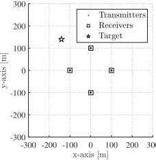
Figure 1. Sensor and target geometry in the surveillance area.

full up and full down chirps respectively. The third waveform is a two-third up and one-thirds down chirp while the fourth is a one-third up and two-thirds down chirp. The reason of choosing this specific design is to achieve low cross-correlation between all the waveforms while occupying all the available bandwidth. In this case the lower and higher cross-correlation maxima between the waveforms are −34.6and−27dB.

For the geometry of the system, the transmitters and receivers are placed in pairs on a circle with 50 m radius centred at the centre of the surveillance area. Lastly, the received signal is calculated for a target with a centre of mass placed at x0 = [−140,140]m and velocity v0 = [0,0]m/s.

The geometry of the described system can be seen in Figure 1.

A. Scenario 1

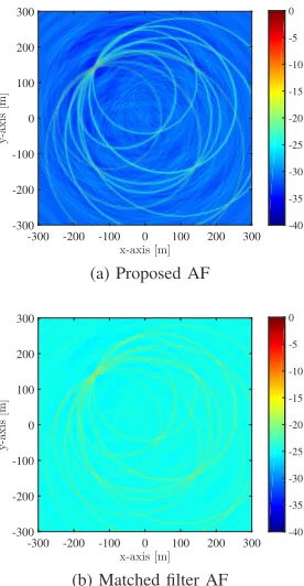
In the first scenario the above system is examined using the generalised mustistatic AF. It is also assumed that all transmitters use the same power and the total energy consumed by the system is 10 MW. This places the target at the very high SNR of tr [SNR_{θ0] = 37 dB. While this might not}

[image:5.612.374.488.55.172.2]

be realistic for a typical radar localisation problem, the high SNR is useful for better understanding the behavior of the AF. Figure 2 illustrates the resulted multistatic AF in logarithmic scale using the proposed formulation (see sub-figure (a)) and by squaring the summation of the matched filtered outputs at each receiver and dividing by the maximum value (see sub-figure (b)). As it can be seen in Figure 2a the maximum of the proposed AF can be used for target localisation. Additionally, stronger ambiguities can be noticed at the circles and ellipses associated with the target’s delay bins for the monostatic and bistatic radars pairs respectively. In Figure 2b on the other hand very strong ambiguities can be observed on areas close to the transceivers.

B. Scenario 2

The second examined scenario follows the same configu-ration as in the Scenario 1 with however the energy parameter

x-axis [m]

-300 -200 -100 0 100 200 300

y

-ax

is

[m

]

-300 -200 -100 0 100 200 300

-40 -35 -30 -25 -20 -15 -10 -5 0

(a) Proposed AF

x-axis [m]

-300 -200 -100 0 100 200 300

y

-ax

is

[m

]

-300 -200 -100 0 100 200 300

-40 -35 -30 -25 -20 -15 -10 -5 0

[image:6.612.377.515.54.320.2]

(b) Matched filter AF

Figure 2. Multi-static AF of the described system for Scenario 1 using (a) the proposed formulation and (b) by squaring the summation of the matched filter outputs at each receiver.

and false alarm. It should also be pointed that the localization performance has been significantly improved in both cases compared to the Scenario 1. Comparing Figures 2a and 3a lower ambiguities and floor levels can be observed for the constant energy parameter case.

V. CONCLUSION

In this work a novel multi-static AF is presented based on the Kullback directed divergence applied in a distributed MIMO radar systems framework. Theoretical analysis showed that the AF is maximally stretched between 0 and 1 while also being flexible for various system assumptions. Additionally a performance analysis of a4×4MIMO sensor system was held by comparing the proposed method with the typical approach of adding all the matched filtered outputs at the receivers. The simulation results demonstrated that the proposed method performs significantly better for varying energy parameter and offers lower floor levels when constant energy parameter is assumed.

ACKNOWLEDGMENT

This work was supported by the Engineering and Phys-ical Sciences Research Council (EPSRC) Grant number EP/K014307/1 and the MOD University Defence Research Collaboration in Signal Processing.

REFERENCES

[1] N. Levanon and E. Mozeson,Radar Signals. NY: JohnWiley&Sons, 2004.

[2] A. Haimovich, R. Blum, and L. Cimini, “Mimo radar with widely separated antennas,”Signal Processing Magazine, IEEE, vol. 25, no. 1, pp. 116–129, 2008.

x-axis [m]

-300 -200 -100 0 100 200 300

y

-ax

is

[m

]

-300 -200 -100 0 100 200 300

-40 -35 -30 -25 -20 -15 -10 -5 0

(a) Proposed AF

x-axis [m]

-300 -200 -100 0 100 200 300

y

-ax

is

[m

]

-300 -200 -100 0 100 200 300

-40 -35 -30 -25 -20 -15 -10 -5 0

[image:6.612.106.245.54.320.2]

(b) Matched filter AF

Figure 3. Multi-static AF of the described system for Scenario 2 using (a) the proposed formulation and (b) by squaring the summation of the matched filter outputs at each receiver.

[3] J. Li and P. Stoica, “Mimo radar with colocated antennas,” Signal

Processing Magazine, IEEE, vol. 24, no. 5, pp. 106–114, Sept 2007.

[4] I. Bekkerman and J. Tabrikian, “Target detection and localization using mimo radars and sonars,” Signal Processing, IEEE Transactions on, vol. 54, no. 10, pp. 3873–3883, Oct 2006.

[5] E. Fishler, A. Haimovich, R. Blum, L. Cimini, D. Chizhik, and R. Valen-zuela, “Spatial diversity in radars-models and detection performance,”

Signal Processing, IEEE Transactions on, vol. 54, no. 3, pp. 823–838,

March 2006.

[6] J. Li and P. Stoica,MIMO Radar Signal Processing. NY, USA: Wiley, 2009.

[7] N. Lehmann, A. Haimovich, R. Blum, and L. Cimini, “High resolution capabilities of mimo radar,” inSignals, Systems and Computers, 2006.

ACSSC ’06. Fortieth Asilomar Conference on, Oct 2006, pp. 25–30.

[8] G. San Antonio, D. Fuhrmann, and F. Robey, “Mimo radar ambiguity functions,” Selected Topics in Signal Processing, IEEE Journal of, vol. 1, no. 1, pp. 167–177, June 2007.

[9] T. Derham, S. Doughty, C. Baker, and K. Woodbridge, “Ambiguity func-tions for spatially coherent and incoherent multistatic radar,”Aerospace

and Electronic Systems, IEEE Transactions on, vol. 46, no. 1, pp. 230–

245, Jan 2010.

[10] M. Radmard, M. Chitgarha, M. Nazari Majd, and M. Nayebi, “Ambigu-ity function of mimo radar with widely separated antennas,” inRadar

Symposium (IRS), 2014 15th International, June 2014, pp. 1–5.

[11] H. Chen, Y. Chen, Z. Yang, and X. Li, “Extended ambiguity function for bistatic mimo radar,”Systems Engineering and Electronics, Journal of, vol. 23, no. 2, pp. 195–200, April 2012.

[12] M. Rendas and J. Moura, “Ambiguity in radar and sonar,” Signal

Processing, IEEE Transactions on, vol. 46, no. 2, pp. 294–305, Feb

1998.

[13] S. Kullback,Information theory and statistics. Courier Corporation, 1968.

[14] M. D. Petkovi and P. S. Stanimirovi, “Generalized matrix inversion is not harder than matrix multiplication,”Journal of Computational and