Multispectral Image Processing for Navigation Using Low Performance Computing

City, University of London Institutional Repository

Citation:

Ronado, D., Aouf, N. ORCID: 0000-0001-9291-4077 and Dubois-Matra, O.

(2018). Multispectral Image Processing for Navigation Using Low Performance Computing.

Paper presented at the 69th International Astronautical Congress (IAC), 1-5 Oct 2018,

Bremen, Germany.

This is the accepted version of the paper.

This version of the publication may differ from the final published

version.

Permanent repository link:

http://openaccess.city.ac.uk/22017/

Link to published version:

Copyright and reuse: City Research Online aims to make research

outputs of City, University of London available to a wider audience.

Copyright and Moral Rights remain with the author(s) and/or copyright

holders. URLs from City Research Online may be freely distributed and

linked to.

City Research Online:

http://openaccess.city.ac.uk/

[email protected]

IAC–18–C1.IP.3

Multispectral Image Processing for Navigation Using Low Performance Computing

Duarte Rondaoa_{, Nabil Aouf}a_{, Olivier Dubois-Matra}b

a _{Centre for Electronic Warfare, Information and Cyber, Cranfield University, Defence Academy of the United}

Kingdom, Shrivenham, SN6 8LA, United Kingdom, {d.rondao, n.aouf}@ cranfield.ac.uk

b_{European Space Agency, ESTEC, Keplerlaan 1, 2201 AZ Noordwijk, Netherlands, [email protected]}

_{Corresponding Author}

Abstract

Space debris represents a growing threat for both current spacecraft and future launches. This is exceptionally alarm-ing in the case of low Earth orbits, where chain impacts of existalarm-ing debris generate even more fragments, increasalarm-ing the probability of further collisions. The now defunct satellite Envisat represents one of the largest objects classified as space debris. The e.Deorbit mission will demonstrate active debris removal (ADR) technology to successfully decom-mission Envisat and other non-functional target spacecraft in orbit. Relative navigation solutions shall be achieved using image processing algorithms, which implies the detection and matching of two-dimensional regions of inter-est. In this work, multiple pattern recognition techniques are investigated for the detection and description of these features. This analysis of feature perception is achieved for the first time in the context of space non-cooperative rendezvous (NCRV) across two different modalities: the visible (0.39-0.70 µm) and the thermal infrared (8-14 µm). The assessed algorithms are implemented in a dedicated, space-appropriate hardware processor to benchmark their real-time capabilities.

Keywords:Active Debris Removal, Multispectral, Feature Detection, Local Descriptor, Space Navigation, Real-Time

Acronyms/Abbreviations

ADRactive debris removal

BBBBeagleBone(R) Black

BRISKBinary Robust Invariant Scalable Keypoints

CenSurECentre Surround Extrema

DoGDifference of Gaussians

FASTFeatures from Accelerated Segment Test

FREAKFast Retina Keypoint

GFTTGood Features To Track

IPimage processing

IRinfrared

LIOPLocal Intensity Order Pattern

LoGLaplacian of Gaussians

LVLHlocal-vertical-local-horizontal

NCRVnon-cooperative rendezvous

NNDRnearest-neighbour distance ratio

ORBOriented FAST and Rotated BRIEF

ROCreceiver operating characteristic

SFMstructure from motion

SIFTScale-Invariant Feature Transform

SLAMsimultaneous localisation and mapping

SURFSpeeded-Up Robust Features

1. Introduction

Space debris consists of the collective inoperative man-made objects currently orbiting the Earth. It represents a growing threat for both current spacecraft and future launches, as it is estimated that nearly 85 % of current space objects are classified as space waste [1]. Indeed, it has now been shown that this growth is being fuelled by chain reactions of collisions among objects that started as far back as 2007, a phenomenon which is termedKessler syndrome. This fact justifies that debris mitigation strate-gies must be applied efficiently, whereas international rules state that at least five large space objects per year must be de-orbited in order to ensure long-term space op-erations [2].

One such strategy is termed ADR, where a chaser spacecraft is deployed to perform a NCRV with the target object in order to capture and de-orbit it. Thee.Deorbit missionis set to be the first ADR mission to be carried out by the European Space Agency (ESA), demonstrating the removal of a large ESA-owned object from its cur-rent orbit and performing a controlled re-entry into the at-mosphere. The Envisat spacecraft, launched on 1 March 2002 and non-functional since 9 May 2012, is a possible

IAC–18–C1.IP.3 Page 1 of 11

https://iafastro.directory/iac/paper/id/43502/summary/

target as it is one of the few ESA-owned debris in low Earth orbit, has a heavy mass, and is located in a crowded orbit [3].

e.Deorbit is part of ESA’s CleanSpace initiative, which is focused on outlining the required technology for this domain, including advanced image processing (IP) for the relative navigation aspect of the NCRV. Using low-power-low-cost monocular camera-based systems, two-dimensionalfeaturesof the target image can be identified and extracted to yield a relative navigation solution; in particular, when the target is not known accurately, such as in the case of a defunct satellite damaged by collisions with debris, these features are oftentrackedin time using matching algorithms and processed with visual mapping methods, such as structure from motion (SFM) or simul-taneous localisation and mapping (SLAM). As the space environment may prove hostile to solutions in the visi-ble wavelength due to illumination, approaches to ADR in other spectra have been proposed, such as the thermal infrared (IR) [4].

Whereas studies comparing the general performance of IP algorithms in the visible [5–7] and in the thermal in-frared [8] are present in the literature, fewer exist which apply it in a space NCRV context [9], and none were found to do so in the infrared domain. Therefore, the pur-pose of this paper is to benchmark the performance of IP techniques adjusted towards multispectral camera setups than can be inserted in space rendezvous missions using affordable, low performance computing.

The structure of this paper is organised as follows. In Section 2, a background of image processing given, which includes a description of the assessed algorithms as well as the figures of merit used to benchmark them. Section 3 describes the devised experimental setup, namely the details of a new multispectral dataset generated for this experiment and the outline of the implementation of the performance analysis tool. Section 4 showcases and dis-cusses the attained results with the tool. Lastly, Section 5 presents the conclusions of the study.

2. Background

Each relative navigation mission using imaging sys-tems must consider performance figures to assess the vi-ability of the IP algorithms used. This section analyses these figures of merit for the selected feature detectors and descriptors operating on the visible and thermal infrared spectra in the devised scenario, and provides a theoretical background for these algorithms.

2.1 Feature Detectors

The analysed detectors can be classified into two groups. The first group consists ofcorner detectors, i.e.

algorithms that extract points defined as the intersection of two edges. The Harris corner detector [10], a his-torically influential algorithm in computer vision, works through the minimisation of the auto-correlation function that compares an image patch against itself shifted for small increments. Harris and Stephens showed that this is equivalent to testing the pair of eigenvalues of the auto-correlation matrix for a candidate point: if both are suffi-ciently large, it corresponds to a minimum in the function and hence to a corner that can be tracked reliably. The test itself is implemented through a corner response func-tion that depends on an empirical constant and quadrati-cally on the eigenvalues; the point is then selected if the response is greater than a given threshold. The Good Fea-tures To Track (GFTT) algorithm [11] improves on the previous method by defining a different corner response function: since the larger uncertainty component in the location of a matching patch is in the direction corre-sponding to the smallest eigenvalue, the proposed corner response function is merely dependent on it. Research continued to evolve in the sense of devising swift inter-est point detection methods. One such algorithm is Fea-tures from Accelerated Segment Test (FAST) [12], which is based on analysing the intensity of a fixed number of pixels around a candidate. FAST makes use of ma-chine learning techniques by having built a decision tree from alternative training images that suggests which pix-els should be assessed first on the test images in order to exclude a large number of non-corners, hence improving detection speed.

approximat-(a) (b)

Fig. 1: The difference of Gaussian pyramid structure. (Reproduced from [14]) (a) Adjacent Gaussian images are subtracted to produce the DoG images, each octave is characterised by downsampling the previous one by a factor of 2 (b) Features are selected in the DoG images by comparing a candidate point (X) to its neighbours (green)

ing the LoG. The former utilises box filters, which can be evaluated swiftly independently of size using integral im-ages, whereas the latter employs bi-level center-surround filters that mitigate subsampling accuracy effects at larger scales.

2.2 Feature Descriptors

The present work considers threefloating pointtype, or distribution-based, descriptors and three binary type descriptors. Distribution-based descriptors are called as such since they encode (in a floating point vector) how certain elements of the support region to the feature point are distributed around it. The first considered descriptor of this type, Scale-Invariant Feature Transform (SIFT) [14], calculates a histogram of local oriented gradients for each 44 subregion around the keypoint. Each histogram has a resolution of 8 bins, giving the descriptor vector a size of 128 elements (Fig. 2a). The Speeded-Up Robust Fea-tures (SURF) algorithm [15] proposes a refinement to this process by computing instead the Haar wavelet responses and storing them in a four-dimensional descriptor vector for each subregion, making up for a total of 64 elements. The more recent Local Intensity Order Pattern (LIOP) de-scriptor [17] is also benchmarked: the overall intensity order (i.e. the order acquired by sorting pixels by increas-ing intensity) is used to divide the local patch into subre-gions labelled ordinal bins; a LIOP of each point is de-fined based on the relationships among the intensities of its neighbouring sample points inside each bin; lastly, the descriptor for the patch is constructed by concatenating the LIOPs of each bin together.

The second type of considered local feature descrip-tor differs from the previous one in the sense that, in-stead of using a floating point vector representation, each

descriptor consists of a binary string. For each feature point, a binary descriptor typically samples sets of pixel pairs px1,x2qi, i P nfrom the support patch, and per-forms a simple intensity comparison, where the result is

1 if Ipx1q   Ipx2q, and 0 otherwise, generating an n-dimensional bit string. To this end, Oriented FAST and Rotated BRIEF (ORB) [18] favours an isotropic Gaussian distribution pattern, rotated according to the orientation of the extracted feature. The algorithm used a training phase consisting of a greedy search algorithm to go through all the possible binary tests and select those that maximise the variance of the descriptor vector. Binary Robust Invariant Scalable Keypoints (BRISK) [19] applies a sampling pat-tern made up ofnlocations equally spaced on circles con-centric with the interest point (Fig. 2b). Two subsets are defined in accordance with two scale-proportional thresh-olds: one of short-distance pairings and another of long-distance pairings. The gradients of the long-long-distance pairs are used to compute the overall characteristic pattern di-rection of the feature. After that, the pattern is rotated ac-cordingly and the binary descriptor string is assembled by performing all the short-distance intensity comparisons of pixel pairs. This allows a single point to take part in more comparisons, limiting the complexity of the intensity val-ues look-up process. Fast Retina Keypoint (FREAK) [20], on the other hand, adopts the human retinal sampling grid as the sampling pattern for the pixel intensity compar-isons: it is a circular geometry where the density of points drops exponentially from the centre outwards, mimick-ing the spatial distribution of ganglion cells in the eye. A coarse-to-fine pair is shown to yield the largest vari-ance and uncorrelation between pairs, i.e. the first selected pairs compare sampling points in the outer circles and the last pairs compare points in the inner circles. The first 16 bytes encode the coarse information, which is applied as a triage in the matching process, accelerating the procedure even further.

Table 1 highlights the differences between the descrip-tor types. Note that many of these algorithms were de-signed for detection as well as description. Indeed, DoG and Fast-Hessian are part of SIFT and SURF, respectively, and ORB and BRISK both use a FAST-based method for feature detection in their original implementations.

2.3 Performance Metrics

thresh-(a)

−15 −10 −5 0 5 10 15 −15

−10 −5 0 5 10 15

(b)

Fig. 2: Distribution-based and binary description. (a) SIFT: the gradient magnitude and orientation at each sub-region are weighted by a Gaussian window (blue) and ac-cumulated into a histogram (reproduced from [14]) (b) BRISK: sampling locations (blue) and Gaussian kernels to smooth intensity values (red) forn60points (repro-duced from [19])

Table 1: Descriptors characteristics. (Adapted from [7])

Descriptor Data Type # Elements Size [bytes] Matching Type

SIFT Floating point 128 512 Euclidean norm SURF Floating point 64 256 Euclidean norm LIOP Floating point 144 576 Euclidean norm

ORB Binary 256 32 Hamming norm†

BRISK Binary 512 64 Hamming norm

FREAK Binary 512 64 Hamming norm

†_{The Hamming distance between two strings of equal length is defined as the minimum number}

of substitutions required to convert one into the other.

old (Fig. 3). Formally, the following condition must hold:

1RMaXRpHTMbHq

RMaYRpHTMbHq

 ε0, (1)

where RM represents the elliptic region defined by

xT_{M x 1andε0 is the overlap error threshold. This} mapping, the ground truth, can be given by a 33 homog-raphy matrixH, assuming a pinhole camera model and that the two related images represent same planar surface in space.

Consequentially, the repeatability score for a given pair of images is calculated as the ratio between the num-ber of correspondences and the numnum-ber of total features presented in the reference image:

repeatabilityC

C . (2)

A second type of testing performed is based on the

matching score. This test verifies how well the regions can be algorithmically matched, thus assessing the dis-tinctiveness of the detected regions. To this end, a de-scriptor for the regions is computed and the total matches M provided by it are checked to see if they agree with the correspondences obtained withH. If a matched pair

f1 f2

H

Fig. 3: The homography ground truth H maps the red feature from framef2to framef1. The overlap area with the original blue feature fromf1is shown in green. If the amount of green is above a certain defined threshold, then the two features correspond.

is also a correspondence, then it is deemed a correct match M , contributing to the matching score as

matching score C XM

C

M

C . (3)

To put it in short, features are desired to be repeatable, i.e. the same features should be observed regardless of how the target is manipulated, but they should also be dis-tinctive enough so that they can be matched regardless of those transforms.

To evaluate the performance of feature descriptors, the figures of recall and precision are used. Recallis defined as the ratio of correct matches to the number of correspon-dences between a pair of frames:

recall M

C . (4)

On the other hand, precision is the ratio of correct matches to the total number of matches:

precision M

M. (5)

to the second nearest neighbouring descriptors is below a certain thresholdµ:

NNDR}DbDa}

}DcDa}  

µ, (6)

whereDb, Dcare the first and second nearest neighbours toDa, respectively. Results from [6, 8] show that using a NNDR improves the matching precision relative to other strategies.

The performance of different descriptors is often com-pared by generating for each one sets of recall and 1-precision values with varying values ofµ. The plotted points result in a receiver operating characteristic (ROC) curve [21]. The larger the area under a descriptor’s ROC curve, the better its performance, providing an intuitive way to benchmark descriptors.

The average computation times per extracted and de-scribed feature are benchmarked, respectively, for each detection and description algorithm. This assumes a pro-portionality between the required time and the computa-tion burden, which can then be of interest to make an in-formed choice on the algorithm for a given application.

3. Experimental Setup

In this section, the experimental setup arranged to eval-uate the performance of the IP algorithms is described. The generated datasets are delineated, and details of the implementation of the algorithms are outlined.

3.1 Dataset

A chaser spacecraft is assumed to approach the tar-get with the translational profile relative to the local-vertical-local-horizontal (LVLH) reference frame illus-trated in Fig. 4. The spin axis of the target in the body frame is aligned with the Y saxis, and the spin axis in the LVLH frame is aligned with the Hbar axis. The chaser assumes a constant orientation with regards to the target’s LVLH frame. The sequence begins with the chaser in a hold point (PH)100 maway from the target. The rendezvous sequence is performed through a forced translationHbar approach (FT) with the target until a stop point (PS) is reached at20 mdistance, after which the sequence ends. This ensures an approximate planarity of the scene between consecutive image frames, allowing the computation of the ground truth using a homography (Section 2).

The current orbit of Envisat is estimated using the two-line element (TLE) data of 30 October 2017. This

_{TLE data obtained from NORAD Two-Line Element Sets Current Data} http://www.celestrak.com/NORAD/elements/

Z

s

X

s

Y

s

(a)

-40 -30 -20 -10 0 10 20 30 40 V-bar

-20 0 20 40 60 80 100 120

H-bar

PH FT PS

(b)

Fig. 4: Scenario specifications for dataset generation. (a) Envisat body reference frame axes (b) Chaser trajectory relative to target LVLH frame

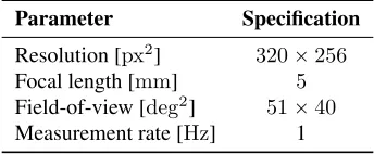
Table 2: Camera properties.

Parameter Specification

Resolution [px2_{] 320256}

Focal length [mm] 5

Field-of-view [deg2_{] 5140}

Measurement rate [Hz] 1

sponds to a situation where the target spacecraft is in full sunlight.

The chaser has two body-mounted cameras in a monocular setup facing the target, one capturing images in the visible band (0.39-0.70 µm) and the other in the thermal infrared (8-14 µm). A 3D computer aided design (CAD) model of Envisat is used to generate the synthetic dataset. The original textured model was heavily modified to guarantee a realistic simulation in the visible spectrum. This included re-meshing the main body of the spacecraft to emulate a “crumpled” effect for the multi-layer insula-tion and adding reflective effects to the solar panel. A sec-ond model was created embedded with material tempera-ture and emissivity for thermal infrared simulation based on the analysis by Ref. [4], where it is assumed that the temperature of each component has reached a steady state. The relative trajectory is imaged using the Astos Cam-era Simulator software. In total, a camCam-era sequence of 200 frames is generated for each of the two modalities. The characteristics of the cameras are displayed in Table 2. Samples of generated images and of detected features are illustrated in Fig. 5. The number of plotted features is limited to 20 for clarity.

3.2 Implementation

The performance analysis framework was coded in the C++ programming language. The OpenCV:library,

(a) (b)

(c) (d)

(e) (f)

Fig. 5: Examples of detected features (green) on frames from the dataset. Left: visible modality. Right: thermal infrared modality. (a, b) Harris (c, d) DoG (e, f) Fast-Hessian

sion 3.3, was used for computer vision and image process-ing related functions.

The native implementations for the Harris, GFTT, DoG, Fast-Hessian, and FAST algorithms are used. For CenSurE, an OpenCV emulation of the original algorithm termed “Star”, was considered. For the descriptors, the native implementations were used for all but LIOP, which was not available. Instead, the original author’s own code; was ported manually into the present framework.

The ground truth homographies mapping each frame to the previous one in the sequence are computeda priori

using the enhanced correlation coefficient (ECC) maxi-mization algorithm [22].

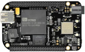
To verify the computing performance of the IP meth-ods, these were implemented and tested on a Beagle-Bone(R) Black (BBB) single-board computer with a

1 GHz ARM Cortex-A8 processor and 512 MB DDR3 RAM (Fig. 6 and Table 3).

;_{https://github.com/foelin/IntensityOrderFeature}

Fig. 6: The BeagleBone(R) Black wireless single board computer.

Table 3: BeagleBone(R) Black properties.

Parameter Specification

System on a Chip (SoC)

AM3358/9

CPU Cortex-A81 GHz

Digital Signal Processor

N/A

On-board storage

8 bit eMMC (running Ubuntu 16.04), microSD card 3.3 V

supported

Memory 512 MBDDR3

Size 86.40 mm53.3 mm

Power ratings 210–460 mAat5 V

4. Results and Analysis

In this section, the results of the adopted framework to determine the performance of the algorithms on the mul-tispectral dataset are delineated.

The different parameters that have a potential influence on the algorithms’ benchmarking setup was analysed a priori. In particular, the following variables were tuned: the overlap error threshold, the normalised region size, and the number of extracted features. The significance of the first variable stands on the fact that it decides how strict the definition of a correspondence is. The impor-tance of the second parameter is related to the fact that the tool could favour detectors with large regions in terms of the repeatability score, so normalising each region size prior to the computation of the features of merit ensures a fairer setup to compare the detectors. The last property is considered to avoid bias towards dense responses, since each detector would extract a different number of features if this tuning was otherwise neglected.

4.1 Benchmarking of Feature Detectors

0 50 100 150 200 Frame 0 20 40 60 80 100 Re pe at abi li ty [% ] Harris GFTT DoG F-Hess FAST CenSurE (a)

0 50 100 150 200 Frame 0 20 40 60 80 100 M at chi ng S core [% ] Harris+LIOP GFTT+LIOP DoG+LIOP F-Hess+LIOP FAST+LIOP CenSurE+LIOP SIFT SURF (b)

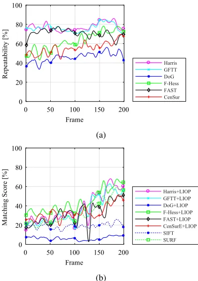
Fig. 7: Performance for rendezvous sequence: visible band. (a) Repeatability (b) Matching score. The raw data is presented smoothed with markers added for readabil-ity. The dashed lines show the results for DoG and Fast-Hessian with their original descriptor

LIOP descriptor. This descriptor was chosen as it is inde-pendent from all the detectors considered. Since the goal is to study the performance of the different feature ex-traction processes, this avoids any bias towards a specific detector, allowing for the examination of the features’ dis-tinctiveness regardless of the chosen descriptor. For added comparison, the performance using the original descrip-tors for DoG and Fast-Hessian (SIFT and SURF, respec-tively) is also showcased to benchmark the full original algorithms and provide a baseline.

An overlap error threshold of 30%, a normalised region size of7.5 px, and a fixed number of 75 extracted features for each detector are considered.

The benchmarks are plotted in Figs. 7 and 8. Consecu-tive image transforms, which are commonly done in SFM and visual SLAM algorithms, are analysed; in this case, a value pertaining to framekin the plot is referent to the transformation between frameskandk 1.

Visible Modality Fig. 7 showcases the performance

of the detection algorithms for the approach sequence in the visible wavelength during a sunlight period. Harris,

0 50 100 150 200

Frame 0 20 40 60 80 100 Re pe at abi li ty [% ] Harris GFTT DoG F-Hess FAST CenSur (a)

0 50 100 150 200 Frame 0 20 40 60 80 100 M at chi ng S core [% ] Harris+LIOP GFTT+LIOP DoG+LIOP F-Hess+LIOP FAST+LIOP CenSurE+LIOP SIFT SURF (b)

Fig. 8: Performance for rendezvous sequence: thermal infrared band. (a) Repeatability (b) Matching score. The raw data is presented smoothed with markers added for readability. The dashed lines show the results for DoG and Fast-Hessian with their original descriptor

GFTT, and FAST achieve the highest repeatability scores. However, in terms of matching scores, they are compara-ble to Fast-Hessian and CenSurE, where the former actu-ally outperforms the rest towards the end of the sequence, showing a bias in favour of shorter target ranges. Con-versely, the matching scores when using GFTT and FAST actually decrease as the chaser nears the target, meaning that the high repeatability attained was likely due to ac-cidental overlapping of features. This could represent a problem when using these detectors with visible imagery at close proximity. CenSurE is the most consistent algo-rithm throughout. Note from Fig. 7b that Fast-Hessian shows a better performance when coupled with LIOP than when combined with its native descriptor. On the other hand, DoG when used with its native SIFT is shown to perform the worst.

Fast-Hessian, and CenSurE) and matching scores increas-ing with time. Note that FAST shows significant declines in the matching score despite its high repeatability, illus-trating lower feature distinctiveness when compared with the other corner detectors. Fast-Hessian again scores one of the highest benchmarks in general.

4.1.1 Discussion

Despite being imaged in two different modalities, the two sequences analysed include common relative motion. Therefore, some similarities in the results are expected. The repeatability, in particular, is comparable for both se-quences. The same cannot be said about the matching scores, however: despite scoring generally lower than the repeatability, they vary in trend and relative ranking be-tween sequences. This highlights the importance in using descriptors to compute matches instead of relying on the geometry overlap only, and implies different degrees of distinctiveness in extracted features depending on the de-tector and wavelength considered.

Corner detectors score higher in repeatability. How-ever, they are often equalled or even surpassed by the blob detectors in terms of matching score. Despite high re-peatability, FAST is one of the least distinctive algorithms across both tests. Fast-Hessian performs well in terms of matching scores in both cases despite average repeatabil-ity. This suggests an extraction of quite distinctive fea-tures, which confirms what was stated in the thermal IR analysis of Ref. [8] and extends the conclusions to the visible spectrum. This is an important finding as it is de-sirable to have a detector that works well in both spectra. DoG shows low scores regardless of the wavelength, but seems to perform worse on the IR. It performs better with SIFT than with LIOP in every situation, whereas Fast-Hessian usually performs better with LIOP than SURF. This reiterates the importance of testing detectors and de-scriptors separately to avoid any cause of bias.

Corner detectors are shown to lose in performance when the target is closer on the visible. This could sig-nify that they are more sensitive to noise coming from the multi layer insulation, for example, as they perform quite well on the textureless IR. In the latter case, the “physical” corners are more evident and impervious to illumination changes.§On the same note, performance is generally bet-ter for the thermal IR case: CenSurE and Fast-Hessian, in particular, are comparable to the visible case, but the for-mer performs better than its visible counterpart in the end of the sequence where the latter does so in the beginning of it.

§_{The reader is reminded that a steady-state thermal condition was}

con-sidered for the IR sequence.

4.2 Benchmarking of Feature Descriptors

For this test, the performance of the descriptors is as-sessed. To this end, a comparison is done using the same feature detector for all the descriptors in order to reduce the influence of the former on the results. Similar settings as in the previous experiments were used, that is, an error threshold of 30% and a fixed number of 75 extracted fea-tures. The regions are not normalised in the computation of the descriptors.

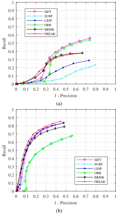
The efficiency of the algorithms is evaluated by com-puting their ROC, or recall/1-precision, curves. Two sets of results are shown for each sequence: the first is a de-scriptor benchmark for short (sucessive) image transfor-mations using the DoG detector; and the second repeats the same experiment using Fast-Hessian. This allows in-sight into if and how different detector-descriptor combi-nations affect the outcomes. These are plotted in Figs. 9–10.

Visible Modality Fig. 9 illustrates the attained ROC curves for the visible modality during the sunlight pe-riod. It can be seen that the performance of the descriptors depends on the feature detection algorithm used: Fast-Hessian features are shown to yield better precision.

It is interesting to note that SIFT performs better with Fast-Hessian features (Fig. 9b) than with DoG features (Fig. 9a). Indeed, when DoG features are used, SIFT performs best, followed by ORB and BRISK, and the per-formance of the three descriptors is comparable.

For Fast-Hessian features, BRISK, FREAK, and LIOP give the best results. Overall the results obtained for SURF are sub-par, showing that combining a feature de-tector with a non-native descriptor can yield better results.

Thermal IR Modality Here, the descriptors are

com-pared for the case of the thermal infrared imaging of the sequence during sunlight conditions; the results are shown in Fig. 10. The performance computed on DoG fea-tures follows the same trend as for the visible case, albeit with a lower yielded precision, which signifies more false matches.

On the other hand, when using Fast-Hessian features the descriptors perform better than for the visible case, in general. FREAK obtains the highest score, but as in the visible case, it behaves quite similarly to BRISK, SIFT, and LIOP. SURF and ORB plot similar curves to their visible counterparts, indicating that they are robust to changes in frequency when computed on Fast-Hessian features.

4.2.1 Discussion

0 0.1 0.2 0.3 0.4 0.5 0.6 0.7 0.8 0.9 1 1 - Precision

0 0.1 0.2 0.3 0.4 0.5 0.6 0.7 0.8 0.9 1

Recall

SIFT SURF LIOP ORB BRISK FREAK

(a)

0 0.1 0.2 0.3 0.4 0.5 0.6 0.7 0.8 0.9 1 1 - Precision

0 0.1 0.2 0.3 0.4 0.5 0.6 0.7 0.8 0.9 1

Recall

SIFT SURF LIOP ORB BRISK FREAK

(b)

Fig. 9: Descriptor ROC curves for the visible band, hot case. (a) DoG features (b) Fast-Hessian features

Fast-Hessian performs better in general both in terms of recall and precision scores, regardless of the modality. As theorised by Ref. [8], a possible explanation for this could be the fact that Fast-Hessian usually extracts larger blobs than DoG, so a larger support area is considered in the computation of the descriptor, capturing in principle a larger signal variation. In can be seen by inspecting Fig. 5 that this is also the case for the analysed dataset.

LIOP was shown to perform better when computed on Fast-Hessian features, both on the visible, and as reported in Ref. [8] on the IR. It can be ranked amongst the best descriptors when used with this type of feature.

Overall, SIFT, BRISK, and FREAK are ranked among the best descriptors for all cases.

4.3 Computation Times

In this subsection, the IP algorithms are benchmarked in terms of their computational performance. These tests

0 0.1 0.2 0.3 0.4 0.5 0.6 0.7 0.8 0.9 1 1 - Precision

0 0.1 0.2 0.3 0.4 0.5 0.6 0.7 0.8 0.9 1

Recall

SIFT SURF LIOP ORB BRISK FREAK

(a)

0 0.1 0.2 0.3 0.4 0.5 0.6 0.7 0.8 0.9 1 1 - Precision

0 0.1 0.2 0.3 0.4 0.5 0.6 0.7 0.8 0.9 1

Recall

SIFT SURF LIOP ORB BRISK FREAK

(b)

Fig. 10: Descriptor ROC curves for the thermal IR band, hot case. (a) DoG features (b) Fast-Hessian features

are ran on the single board computer setup, allowing for the examination of their real-time capacity on a low per-formance embedded system. The recorded benchmarks account only for the core tasks of detection or description. Table 4 portrays the average extraction time per fea-ture for each detector. DoG scores the slowest detection time, at21.2 msper feature. To better compare their per-formance, in addition to the absolute computation times, the relative speed-up factors with respect to the heaviest algorithm are also displayed. FAST is the quickest al-gorithm to run, being almost three orders of magnitude swifter than DoG. As expected (see Section 2), CenSurE is faster than Fast-Hessian, which is in turn faster than DoG. Surprisingly, GFTT is recorded having a higher ex-ecution time than Harris.

Table 4: Average detection times per feature.

Detector Time [ms] Speed-up

FAST 0.0261 814

CenSurE 1.3189 16

Harris 1.4248 15

GFTT 1.4933 14

F-Hess 2.6338 8

DoG 21.2249 1

Table 5: Average description times per feature.

Descriptor Time [ms] Speed-up

ORB 0.1627 103

BRISK 0.2057 81

SURF 0.7676 22

SIFT 9.4847 2

LIOP 14.5418 1

FREAK 16.7328 1

whereas the other algorithms execute leaving a consider-able amount of time left for allocating other tasks.

Analogously, Table 5 shows the benchmarked com-putation times for the descriptors averaged per feature. While the list is topped by two of the binary descrip-tors, FREAK is actually the slowest algorithm, costing

16.7328 msper feature on average. The high computation time is unusual for a binary descriptor and contradicts the findings of Ref. [8]. The authors of the cited research work benchmark the descriptor computation times on an Intel(R) 64-bit processor, which could suggest limitations or different levels of optimisation of the algorithms in dif-ferent architectures.

LIOP is similar in performance to FREAK, while SIFT is two times faster. The former two algorithms exceed the computational budget, though, while the latter takes up

71 %of it. Surprisingly, the performance of SURF is in the same order of magnitude as ORB and BRISK.

5. Conclusions

This paper found that electing a key detector-description combination that outperforms all others is not an straightforward task, as it comes down to a trade-off mainly between robustness and complexity. However, given the hardware limitations it is possible to point out which IP algorithms are more adequate for the studied scenario. A combination of Fast-Hessian with BRISK is capable of providing adequate performance, both in

terms of matching performance and computational effi-ciency, as it was shown to perform inside the boundaries of the considered frame-rate, taking up little over 20 %

of the computational budget. Hence, this combination could possibly be used for a multispectral navigation al-gorithm, analysing a frame of each modality per cycle, and it would still achieve detection and description with less than half of the budget. Furthermore, the benchmark of Fast-Hessian + BRISK is comparable in both spectra, which is an added advantage as a reduced number of al-gorithms means reduced memory usage.

Given the conducted analysis, it should be noted that other detector-descriptor combinations that comply with the hardware requirements are possible. Recommenda-tions include additional experimentation with algorithms besides the ones tested herein, e.g. ORB with its na-tive descriptor. Future work includes analysing the per-formance of IP algorithms under additional perturbations (e.g. sunlight vs. eclipse) and expanding the analysis to benchmark large image transformations.

6. Acknowledgements

The research work detailed in the present

paper has been funded by ESA contract no.

4000117583/16/NL/HK/as.

The authors would like to thank ESA for access to the Astos Camera Simulator.

References

[1] M. Andrenucci, P. Pergola, and A. Ruggiero, “Active Removal of Space Debris: Expanding Foam Appli-cation for Active Debris Removal,” tech. rep., Uni-versity of Pisa, Aerospace Engineering Department, Italy, 2011.

[2] C. Bonnal, J.-M. Ruault, and M.-C. Desjean, “Ac-tive Debris Removal: Recent Progress and Cur-rent Trends,”Acta Astronautica, vol. 85, pp. 51–60, 2013.

[3] R. Biesbroek, L. Innocenti, A. Wolahan, and S. M. Serrano, “e.Deorbit–ESA’s Active Debris Removal Mission,” in7th_{European Conference on Space}

De-bris, ESA Space Debris Office, 2017.

[4] Ö. Yılmaz, N. Aouf, E. Checa, L. Majewski, and M. Sanchez-Gestido, “Thermal Analysis of Space Debris For Infrared-Based Active Debris Removal,”

[5] K. Mikolajczyk, T. Tuytelaars, C. Schmid, A. Zis-serman, J. Matas, F. Schaffalitzky, T. Kadir, and L. Van Gool, “A Comparison of Affine Region De-tectors,” International Journal of Computer Vision, vol. 65, no. 1-2, pp. 43–72, 2005.

[6] K. Mikolajczyk and C. Schmid, “A Performance Evaluation of Local Descriptors,” IEEE Transac-tions on Pattern Analysis and Machine Intelligence, vol. 27, no. 10, pp. 1615–1630, 2005.

[7] O. Miksik and K. Mikolajczyk, “Evaluation of Local Detectors and Descriptors for Fast Feature Match-ing,” in Pattern Recognition (ICPR), 2012 21st In-ternational Conference on, pp. 2681–2684, IEEE, 2012.

[8] T. Mouats, N. Aouf, D. Nam, and S. Vidas, “Per-formance Evaluation of Feature Detectors and De-scriptors Beyond the Visible,”Journal of Intelligent & Robotic Systems, pp. 1–31, 2018.

[9] N. Takeishi, A. Tanimoto, T. Yairi, Y. Tsuda, F. Terui, N. Ogawa, and Y. Mimasu, “Evaluation of Interest-Region Detectors and Descriptors for Au-tomatic Landmark Tracking on Asteroids,” Trans-actions of the Japan Society for Aeronautical and Space Sciences, vol. 58, no. 1, pp. 45–53, 2015.

[10] C. Harris and M. Stephens, “A Combined Corner and Edge Detector,” in Alvey Vision Conference, vol. 15, p. 50, Citeseer, 1988.

[11] J. Shi and C. Tomasi, “Good Features To Track,” inProceedings of the 1994 IEEE Computer Society Conference on Computer Vision and Pattern Recog-nition, pp. 593–600, IEEE, 1994.

[12] E. Rosten and T. Drummond, “Machine Learning for High-Speed Corner Detection,” in European Con-ference on Computer Vision, pp. 430–443, Springer, 2006.

[13] T. Lindeberg, “Scale-Space Theory: A Basic Tool for Analyzing Structures at different scales,”Journal of Applied Statistics, vol. 21, no. 1-2, pp. 225–270, 1994.

[14] D. G. Lowe, “Distinctive Image Features from Scale-Invariant Keypoints,”International Journal of Computer Vision, vol. 60, no. 2, pp. 91–110, 2004.

[15] H. Bay, T. Tuytelaars, and L. Van Gool, “Surf: Speeded Up Robust Features,” inEuropean Confer-ence on Computer Vision, pp. 404–417, Springer, 2006.

[16] M. Agrawal, K. Konolige, and M. R. Blas, “Censure: Center Surround Extremas for Realtime Feature De-tection and Matching,” inEuropean Conference on Computer Vision, pp. 102–115, Springer, 2008.

[17] Z. Wang, B. Fan, and F. Wu, “Local Intensity Or-der Pattern for Feature Description,” in2011 Inter-national Conference on Computer Vision, pp. 603– 610, IEEE, 2011.

[18] E. Rublee, V. Rabaud, K. Konolige, and G. Bradski, “ORB: An Efficient Alternative to SIFT or SURF,” in2011 International Conference on Computer Vi-sion, pp. 2564–2571, IEEE, 2011.

[19] S. Leutenegger, M. Chli, and R. Y. Siegwart, “BRISK: Binary Robust Invariant Scalable Key-points,” in2011 International Conference on Com-puter Vision, pp. 2548–2555, IEEE, 2011.

[20] A. Alahi, R. Ortiz, and P. Vandergheynst, “FReAK: Fast Retina Keypoint,” inComputer Vision and Pat-tern Recognition (CVPR), 2012 IEEE Conference on, pp. 510–517, Ieee, 2012.

[21] R. Szeliski, Computer Vision: Algorithms and Ap-plications. Springer Science & Business Media, 2010.