Categorisation of panic disorder by time-frequency methods

(1)

Categorisation of Panic Disorder by Time-Frequency Methods

Hubert Dietl’, Stephan Weiss’

Dept. Electronics

& Computer Science, University of Southampton,

UK

hud,s.ueissQecs.soton.ac.uk

Abstract. Anxiety patients that are presented with neutral and panic disorder triggering stimuli shon. different

event-related brain potentials (ERP) within the electroen-

cephalogram (EEG). In this paper, we investigate this dif-

ference by time-frequency (TF) revealing transforms lead- ing to an identification of a small number of significant parameterising coefficients to be able to differentiate between the presented stimulus categories.

1. I N T R O D U C T I O N

Individuals with panic disorder are characterised by an abnormal fear of certain anxiety connected sen-

sations such as palpitation, breathlessness, or dizzi-

ness [l]. The research into this disorder has led to

studies investigating its symptoms by means of appro- priate stimulation and measurement of the subsequent

ERP [2, 31. In this context, visual stimulation has been

performed with words causing panic disorder, whereby the EEG can be recorded showing event related potentials. Previous studies have resulted in revealing a low frequent transient waveform appearing approximately 300 ms after stimulus onset as a distinctive character-

istic nhich is referred to as P300.

Analysis of variances (ANOVA) [4] is one method

of detecting the P300 in panic disorder and normal re-

sponse ERP. Since the P300 has a transient behaviour,

the application of time frequency (TF) analysis appears

well suited, as it takes both spectral and temporal in-

formation into account 151. In this paper we aim to in-

vestigate various transforms - such as wavelet, wavelet

packet, and Gabor transforms - with respect t o their

suitability for revealing the TF characteristics of the

transient P300. We further optimise these transforms

such that the distinction between panic disorder and normal responses is concentrated in only few transform

coefficients, t o which a statistical test can be applied.

T h e paper is organised as follows. Sec. 2 will intro-

duce the background and experimental conditions un-

der which panic disorder data was obtained. In Sec. 3

suitable TF transforms will be reviewed, which can pa-

rameterise the elicited event related potentials, while

Sec. 4 discusses a method t o isolate indicative param-

eters, which can be used for distinguishing between

panic disorder and normal EEG. Finally, test results

and conclusions are presented in Secs. 5 and 6.

2. P A N I C D I S O R D E R E R P

The panic disorder ERP were measured for an anx-

iety patient who was presented with fear-inducing

or neutral words tachistoscopically at the perception

threshold of panic disorder. The patient’s perception

threshold for correctly identifying 50% of the words v a s

determined with neutral words not used in t,he experi:

ment. It can be assumed that the patient will recognise

a greater number of anxiety words given at his percep-

tion threshold than neutral words [4]. Thus, it can

be expected that the EEG exhibit an difference when neutral and anxiety words are presented.

The EEG was measured at the vertex electrode (Cz)

synchronously t o the stimuli, whereby the recordings

were started 100 ms before the onset of the visual word

st,imulus. The data exemplary analysed in this study

contains 24 neutral word presentations and 24 anxi-

ety word presentations to one panic patient. Fig. 1

shows the average over the stimulus-synchronous EEG

in reaction to the 24 words presented for each word

category. The figure reveals a difference in the two av-

-5 , , , , , , , I

0 O I D l 0 8 0 0 I ,I 1 , , I I 8 2

ameiisi

Fig 1. 4serage over 24 EEG segments showing

(2)

DWT b, Wavelet Packets e ) Gabor Framer

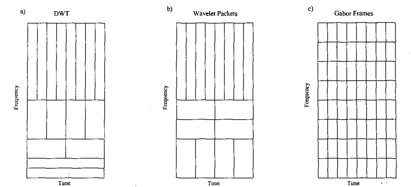
Fig. 2. Time-frequency tiling by a) DIVT, b) a sample \VP decomposition, and c) a G F decomposition.

erages with a stronger P3UU and more positive EEG

until approximately t = 700 ms in the panic disorder

related dat,a.

3. PARAMETERISING TRANSFORMS

To take the transient nature of the ERP waveforms

in Fig. 1 into, account, T F transforms are used for pa-

rameterisation of the data. To capture the impulsive

rise of the P300, T F transforms xvith a good time res-

olution are required. The discrete wavelet transform (DWT) hore\-er generally yields a good frequency resolution and poor time resolution at low frequencies, resulting in a too coarse time segmentat.ion in the frequency range of interest. Therefore, we concentrate on wavelet packet (WP) transform, whose level of decomposition can be adapted t o fit the nature of the data,

as well as the Gabor Frame (GF) decomposition, which

yields a uniform tiling of the T F plane and hence can

provide a desired resolution in a specific TF segment.

Fig. 2 shom an example for the T F characteristics of

the DWT, the W P and the GF.

The W P is based on Mallat's wavelet [5], whereby

the decomposition level of the transformation is

adapted t o minimise the entropy of the average ERP

curves in Fig. 1. The GF decomposition is based on an

oversampled filter bank with a flexible number of chan-

nels constructed according to

[SI,

whereby the channel

number is selected in order to minimise the transform coefficients' entropy when applied t o the average ERP curves. Both transformations are operating on finite length EEG segments and are implemented with sym-

metric boundary extensions [7, 8).

The application of the \VP and G F transforms leads

t o a parameterisation of the E R P data whereby the

features of the E R P are expressed in as few coefficients

as possible. Within these ERP-parameterising coeffi-

cients, those that represent a significant difference be-

tween the two data sets need t o be identified next.

4. DIFFERENCE EVALUATION

Based on the parameterisations introduced in the previous section, we want t o identify coefficients that

allow us to differentiate between the presented anxiety

related and neutral words in this section.

4.1 F-test

Prior t o the selection of significant coefficients that

represent the main characteristics of the data, an F-

test [9] is conducted to determine which method is used

to identify them. The aim of this test is t o determine whether two data sets are sampled from normal dis-

tributions with the same variances.

If

a d u e for the

significance level P of lower than 0.05 is obtained by the

F-test, we conclude that the hypothesis is rejected and the two data sets are sampled from normal distrihu-

tions having different variances. The value of P = 0.05

is a limit commonly used in medical research [9]. Com-

paring sets x, and x, containing the panic disorder

and neutral E R P response coefficients for one specific

transform coefficient across all 24 measurements, the

[image:2.613.115.537.98.290.2]

(3)

with 0; and 0: being the variances of the two data

sets. To receive the significance level P for the F-test,

we need to define the degrees of freedom for the two

data sets according to

up = N , - l a n d

vn = N,, - 1 , (2)

with N p = N,

=

24 being the number of samples, vp

the degrees of freedom for the panic data set and v, the

degrees of freedom for the neutral data set. With the F

value defined by (1) and the degrees of freedom vp and

v,, the significance level P for the F-test can be deter-

mined from lookup tables in literature, e.g. [9]. If the

outcome of the F-test confirms that the two data sets are sampled from distributions with equal iariances,

we can subsequently conduct a t-test t o determine dis-

tinctive coefficients. If the result of the F-test is that the underlying distributions from which the two data groups are sampled possess different variances we con-

duct a ut-test. The t-test and the ut-test are defined

in the next subsection.

4.2 T- and UT-Tests

The t-test gives the probability that two data sets sampled from potentially two different distributions nith identical variance possess different mean values,

for which a significance is returned. The t-value is de-

fined as [IO]

with 0' = u: = u:. The values rtp and if,, represent

the means for the two data sets, according to

The t-value also corresponds t o a certain significance

level P , which can be looked up from tables [lo], with

the degrees of freedom defined by vt = up

+

v, =

Np

+

N, - 2. A smaller value for P indicates that the

data sets have a significantly different mean. For ex-

ample, for P = 0.01 the probability that the differences

in the means are due t o a sampling error is 1%. For

our study, a significance level of P = 0.01 was used t o

identify distinctive coefficients. The two tested distributions were the distributions for a specific transform

parameter over the presented 24 neutral and anxiety

words, respectively.

For the case that the F-test yields a difference in variances such that the t-test cannot be used, we apply

a ut-test for unequal variances defined as

xp

-

F"

U t =

@-$.

(5)

According t o [ll], for data sets sampled from distribu-

tions with unequal variances, the t distribution can be

approximated by the ut value if the t table is entered

at the following defined degree of freedom:

Again, for our study, a significance level of P = 0.01

was used for the ut-test t o identify distinctive coeffi-

cients. This test tends t o be less powerful than the

usual t-test, since it uses fewer assumptions [9]. As it

will be shown in the application in the next section, all identified distinctive coefficients there hare been is-

lated by the t-test. The main purpose of the ut-test

is t o have an analysis tool for all coefficients a t hand

whether they show equal variances or not.

To confirm the results obtained by t-tests or ut-tests, a back test can be performed based on an ROC analysis as shown in the next subsection.

4.3 ROC Analysis

Back

Test

According t o [12], a good measure for differentiation

betn.een two distributions are ROC curves, since the area under the ROC "curve measures the separabilitr independent of the selection of any threshold.

Here, we make use of it t o back test the results ob-

tained by t-tests or ut-tests. The back test is performed

a s follows. For every coefficient received, the area under the ROC curve is measured. For this measure, two Gaussian distributions are generated. From these dis-

tributions, the same number of random samples as in

the preceding t-test or ut-test are taken out and based on a t-test or ut-test, the significance level is calculated for these samples originating from the Gaussian distributions. This calculation is repeated with random samples from the distributions and the significance level is

averaged until it converges. Tab 1 shows some areas

under the ROC curve and their corresponding signifi-

cance levels P .

In most social research a significance level of P =

0.05 is used to determine differences between two sets of data. Therefore, if in our study the area under ROC

curve 1s equal or greater than 0.72, we will conclude

(4)

Area under the ROC curve

)I

Significance level P

0.74

/I

0.028

0.72

0.70

0.046 0.067

Tab. 1. Area under ROC curve and significance

lei-els P .

5. TEST A N D D I S C U S S I O N

As discussed in Sec. 3 and Sec. 4, we have differ-

ent transform methods and a procedure t o identify significant coefficients t o being able to separate between presented neutral and anxiety words. In the following, q-e will discuss the used transforms and present the results for separability which we obtained for the data

described in Sec. 2.

5.1 Transform A d j u s t m e n t

The optimal decomposition structure for the WP

is found over minimising the entropy as described in

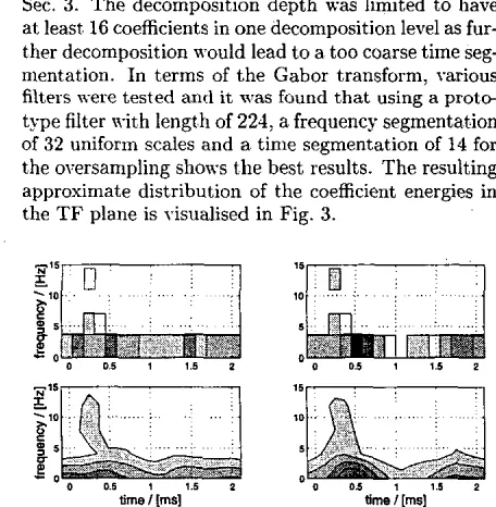
Sec. 3. The decomposition depth was limited to have

at least. 16 coefficients in one decomposition level as fur-

ther decomposition n-ould lead t o a too coarse time segmentat,ion. In terms of the Gabor transform, various

filters were tested and it was found that using a prote

type filter vith length of 224, a frequency segmentat.ion

of 32 uniform scales and a time segmentation of 14 for

the oversampling shows the best results. The resulting approximate distribution of the coefficient energies in

the T F plane is 7-isualised in Fig. 3.

5.2 Identified Coefficients and Difference Com-

parison

The coefficients to which the difference evaluation

is applied were preselected whereby only coefficients

are considered which contain 85% of the total energy.

This is reasonable, as it reduces the probability t o iden-

tify coefficients that contain noise only. The Talue of 85% results from not considering coefficients that are

located above 15

Hz

in the TF plane, see Fig. 3.

Fig. 4 shows the resulting coefficients when perform-

ing the difference evaluation on the parameterised data. We see that two coefficients (black and grey) for both

Fig. 4. Resulting coefficients for (left) WP and

(right) Gabor transforms.

transforms are identified. They cover approximately

the area

of

the P300 slow wave as it is expected in

Sec. 2. They are all identified via a t-test according

to a prior F-test whereby the threshold for the signif-

icance level for the F-test was P = 0.05, and for the

t-test, it was set t o P = 0.01 as mentioned in the pre-

vious section.

Fig. 5 shows the difference of the averages of the

neutral and anxiety EEG compared with its pararne-

terisation by the identified coefficients for the two in- vestigated transforms. It can be observed that the two

identified coefficients parameterise the P300 area very

. . .

0 02 0.4 0.e 0.8 1 13 1" 1.8 4 . 0 2

. . .

* :

.... ... . . . . . .

I 02 1.1 06 o.* I 3 2 1.4 1.6 'd 2

timellsl

Fig. 5. Difference of neutral and anxiety EEG

data compared with its parameterisation by the

two identified coefficients for (tau) WP and (bot-

Fig. 3. Arerage coefficient energy for (left) neutral

words and (right) panic order related words using

(top) WP and (bottom) Gabor transforms.

[image:4.613.97.307.102.149.2] [image:4.613.339.550.259.319.2] [image:4.613.83.311.395.628.2] [image:4.613.336.558.516.640.2]

(5)

well for both transforms. potential,” Journal of Psychophysiology, vol. 6 ,

To show the results of the back test for the identified pp. 285-298,1992.

coefficients, Tab. 2 indicates the ROC curve analysis

for these coefficients. Comparison with Tab. 1 yields

I

II

Transform

1

Coefficient

I/

WP

I

GF

black

11

0.73

I

0.73

I

grey

11

0.72

I

0.72

I

Tab. 2. Area under ROC curve for the identified

coefficients.

that all coefficients obtained show an equal or greater

value than 0.72 and therefore, pass the back test what

justifies the use of the respective transforms. Recapit- ulating, it can be said that with both transforms an adequate separation of data of both categories, namely presented neutral and anxiety words, can be achieved. These results were contrasted t o a difference evaluation applied t o the time domain and frequency dc- main data, where the latter is calculated via a discrete Fourier transform, for which only poor separability was achieved.

6. CONCLUSIONS

We have presented a

W P

and Gabor transforms

analysis comparison for parameterising ERP with the aim of differentiating between presented neutral and anxiety words to a patient with panic disorder. We have motivated the use of T F methods, and proposed a n approach to obtain distinctive transform coefficients, whereby the results were verified by different tests for different cases. It was shown that the presented T F transforms can be used with good results to classify panic disorder via analysis of ERP.

REFERENCES

[4] P. Pauli, G. Dengler, G. U’iedemann, P. Mon-

toya, H. Flor, W. Birbaumer, and G. Buchkremer,

“Behavioral and Neurophysiological Evidence for Altered Processing of Anxiety-Related Words in

Panic Disorder,” Journal of Abnormal Psychol-

ogy, vol. 106, no. 2, pp. 213-220, 1997.

[5] Stephane G. hfallat, “hlultiresolution Approxima-

tions and Wavelet Orthonormal Bases of L2 (R),”

Transactions of the American Mathematical Soci-

ety, vol. 315, no. 1, pp. 69-87, September 1989.

[6]

M.

Harteneck, S. Weiss, and R.

W.

Stewart, “De-

sign of Near Perfect Reconstruction Oversampled

Filter Banks for Subband .4daptive Filters,” IEEE

Bansactions on Circuits €4 Systems

II;

~ o l . 46, no.

8, pp. 1081-1086, August 1999.

171 G. Strang and T. Nguyen, Wavelets and Fil-

ter Banks, Wellesley-Cambridge Press, Wellesley,

MA, 1996.

[SI H. Dietl, S. Weiss, and U. Hoppe, “Compari-

son of Transformation Methods to Determine Fre- quency Specific Cochlear Hearing Loss Based on

TEOAE,” in Digest 02/110 IEE Colloquium on

Medical Applications of Signal Processing, IEE,

London, October 2002, pp. 16/1-16/6.

[9] P. Armitage, G. Berry, and J.N.S. hlat.thens, Sta-

tistical Methods in Medical Research, Blackwell

Science, Oxford, fourth edition, 2002.

[lo] 1.N Bronstein and K . A . Semendjajew, Taschen-

buch der Mathematik, Verlag Harri Deutsch, Thuu

und Frankfurt/Main, 23rd edition, l9S7.

[ll] F.E. Satterthwaite, “An approximate distribution

of estimates of variance components,” Biometrics

Bul1,~wl. 2, pp. 110-114, 1946.

1121 J. A. Hanlev and B. J. McNeil. “The hieanina

, >

-

and Use of the .4rea under a Receiver Operating

Characteristic (ROC) Curve,” Radzology, vol. 143,

pp. 26-36, 1982.

[l] D. M. Clark, “A cognitive approach t o panic,”

Behauiour Research and Therapy, vol. 24, pp. 461-

470, 1986.

[2] E. A. Kostandov and Y. L. Arzumanov, “Average

cortical evoked potentials to recognised and non-

recognised verbal stimuli,” Acta Neurobiologica

Ezperimentalis, vol. 37, pp. 311-324, 1977.

[3] E. Naumann, D. Bartussek, 0. Diedrich, and M.E.

Laufer, “Assessing cognitive and affective infor- mation processing functions of the brain by means