DIRSIG digital imaging and remote sensing imaging generation model: Infrared airborne validation & input parameter analysis

Rochester Institute of Technology

RIT Scholar Works

Theses

Thesis/Dissertation Collections

4-1-1996

DIRSIG digital imaging and remote sensing

imaging generation model: Infrared airborne

validation & input parameter analysis

Todd Kraska

Follow this and additional works at:

http://scholarworks.rit.edu/theses

This Thesis is brought to you for free and open access by the Thesis/Dissertation Collections at RIT Scholar Works. It has been accepted for inclusion

in Theses by an authorized administrator of RIT Scholar Works. For more information, please contact

[email protected]

.

Recommended Citation

DIRSIG

Digital Imaging and Remote

~ensing

Image Generation Model:

Infrared Airborne Validation

&

Input Parameter Analysis

Todd

A.

Kraska

Rochester Institute of Technology

Chester F. Carlson Center for Imaging Science

A thesis submitted in partial fulfillment of the

requirements for the degree of Master of Science

at the Chester F. Carlson Center for Imaging Science

in the College of Science

of the Rochester Institute of Technology

April 1996

Signature of the Author

_

Accepted by

Dana

G.

Marsh

CHESTER F. CARLSON

CENTER FOR IMAGING SCIENCE

COLLEGE OF SCIENCE

ROCHESTER INSTITUTE OF TECHNOLOGY

ROCHESTER, NEW YORK

CERTIFICATE OF APPROVAL

M.S.

DEGREE THESIS

The M.S. Degree Thesis of Todd

A.

Kraska

has been examined and approved by the

thesis committee as satisfactory for the

thesis requirement for the

Master of Science degree

Dr. John Schott, Thesis Advisor

Dr. Robert Fiete

THESIS RELEASE PERMISSION FORM

ROCHESTER INSTITUTE OF TECHNOLOGY

COLLEGE OF SCIENCE

CHESTER F CARLSON CENTER FOR IMAGING SCIENCE

DIRSIG

Digital Imaging and Remote

~ensing

Image Generation Model:

Infrared Airborne Validation

&

Input Parameter Analysis

I, Todd

A.

Kraska, hereby grant permission to the Wallace Memorial Library ofR.I.T. to

reproduce my thesis in whole or in part. Any reproduction will not be for commercial use

of

profit

Signature:

_

9C

,

-DIRSIG

Digital

Imaging

and

Remote

Sensing

Image Generation Model:

Infrared Airborne Validation

&

Input Parameter Analysis

by

Todd A. Kraska

Submitted

to the

Chester F. Carlson Center for

Imaging

Science

in

partial

fulfillment

of

the

requirements

for

the

Master

of

Science Degree

at

the

Rochester

Institute

of

Technology

Abstract

The

civilian and

military

need

for high

resolution

infrared

imagery

has

dramatically

increased in

recent

times.

Regardless

of

the

useror

the need,

infrared

imagery

canprovide unique

information

that

is

not available

in

the

visible region of

the

electromagnetic spectrum.

Just

as

the

need

for

real

infrared

imagery

has

increased,

so

has

the

need

for

computergenerated

infrared

imagery,

also

known

as synthetic

imagery. Synthetic

imagery

is

created

by

mathematically modeling

the "real

world" and

the

imaging

chain,

encompassing everything from

the target to the

sensor characteristics.

The

amount of

faith

that

can

be

placed

in

a synthetic

image depends

on

its

accuracy in recreating

the

real world.

The Digital

Imaging

and

Remote

Sensing

Image Generation Model

(DIRSIG)

at

the

Rochester Institute

of

Technology (RIT)

attempts

to

model

the

real world.

It

creates synthetic

images

through the

integration

ofscene

geometry,

ray-tracer,

thermal,

radiometry,

and sensor submodels.

The focus

of

this

project

lies in evaluating

the

ability

of

DIRSIG

to

recreate

the

imaging

chain andproduce

high

resolution synthetic

imagery.

DIRSIG

synthetic

imagery

of

the

Kodak

Hawkeye

plant and

the

surrounding

area wascompared

to

aerial

infrared

imagery

of

the

same region

using

root mean square error and rank order correlation.

This

comparison

helped

to

validate

the

output

from DIRSIG

and

detect inadequacies

in

the

image

chain model.

In

addition

to

validating

DIRSIG,

a procedure

for optimizing

the

input

parameters,

incorporating

a

sensitivity

analysis,

was

developed. This

reduces

the

time involved

in creating

arealistic andaccurate synthetic

Table of Contents

Abstract

i

Table

of

Contents

ii

List

of

Figures & Tables

iv

1.0

Introduction

1

2.

0

Objectives

4

2.1 DIRSIG Validation

4

2.2 Input Parameter Analysis & Optimization

6

3. 0

Background

8

3

.

1 The

Big

Equation

8

3.2

Alternative

SIG Models

11

3.3 DIRSIG Overview

17

3.3.1

Scene

Geometry

Submodel

17

3.3.2 Ray-Tracer Submodel

19

3.3.3 Thermal Submodel

23

3.3.4

Radiometry

Submodel

24

3.3.5 Sensor Response

and

Modulation Transfer Functions

28

3.3.6 Final Image Generation Review

29

4.0

Technical Approach & Procedure

30

4.1 Validation

of

DIRSIG

30

4.1.1 Radiometric Validation

33

4.1.1.1 Rank Order Correlation

33

4. 1.1.2 RMS Error

34

4. 1

.2

Geometric Validation

35

4.2 Input Parameter

Analysis

& Optimization

37

5. 0

Experimental

41

5.1 Truth

Imagery

Collection

41

5.1.1 Aerial Image Collection

-Image

1

41

5.1.2 Equipment

Specifications-

Image 1

43

5.1.3

Rooftop

Image Collection

Images 2-3

44

5.1.4 Equipment

Specifications-

Image

2-3

45

5.1.5 Image Collection

Summary

47

5.2

Scene

Development &

Synthetic

Image Generation

50

5.2. 1 Terrain Generation

51

5.2.2

Building

Generation

52

5.2.3 Miscellaneous

Object

Creation

56

5.2.4 Meteorological Data

-Weather

&

Atmosphere

57

5.2.5

Sensor

Parameters

& Profile

57

5.2.6

Image

Creation

Summary

58

5.3 DIRSIG

Validation

Results

61

5.3.1 Validation

-Primary

Truth

Imagery

(Bendix line

scanner)

61

5.3.1.1 Material Radiometric

Accuracy

-RMS Error

67

5.3. 1.2

Material

Radiometric

Accuracy

5.3.1.3 Radiometric

Accuracy

-

Complex Phenomena

73

5.3.1.4 Geometric

Accuracy

82

5.3.2 Validation

-

Alternate Truth

Imagery (Inframetrics)

85

5.3.3 Validation

Summary

87

6. 0

Input Parameter

Sensitivity

Analysis

&

Optimization

88

6. 1

Input

Parameter

Sensitivity

Analysis

88

6.1.1 Weather & Atmospheric

Sensitivity

94

6. 1.2 Material Parameter

Sensitivity

102

6.1.3 Time

History

Material Parameter

Sensitivity

110

6.2

Input

Parameter Optimization

114

6.2. 1 Meteorological Parameter Optimization

119

6.2.2 Material Parameter Optimization

120

6.5 Input Parameter

Sensitivity

Analysis & Optimization

Summary

1 26

7. 0

Recommendation

&

Conclusions

127

7.1

DIRSIG

127

7.2

Sensitivity

Analysis & Input Parameter Optimization

129

7.3 Conclusion

130

8. 0

References

131

APPENDIXA

Validation

Analysis

APPENDIX B

DIRSIG Files

APPENDIX

C

AutoCad

Scene

Construction

APPENDIX D

Material Files

Generic

Optimum

Angular Effects

APPENDIX E

Actual Weather Data

10 November 1991

12

October

1995

APPENDIX F

Sensitivity

Analysis

Meteorological

Data

Material

Data

List

of

Figures &

Tables

Figure3.1

-Solar energy

photon paths

8

Figure 3.2

Self-emitted

energy

photon

paths

9

Figure3.3

-

GTVISIT

overview

11

Figure 3.4

Tl

synthetic

scene generation

13

Figure 3.5

DIRSIG

overview

17

Figure 3.6

Facet

material

parameters

18

Figure 3.7

DIRSIG

data

hierarchy

18

Figure3.8

-

Object &

part

bounding

volumes

19

Figure 3.9

Ray-tracer

model

20

Figure 3.10

Solar

history

21

Figure 3.11

Target Interactions

21

Figure 3.12

Ray-tracer

flow diagram

22

Figure 4. 1

Area

of

interest

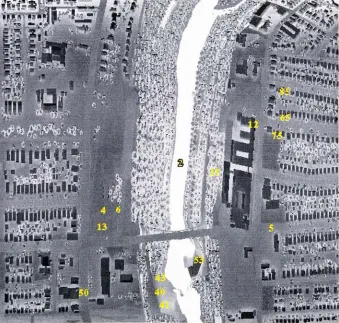
32

Figure 4.2

Relative

minimum

&

maximum

input

values

37

Figure 5.1

-

Piper

Aztec

aircraft

41

Figure 5.2

Line

scanner

image

acquisition

42

Figure 5.3

Bendix

line

scanner

43

Figure 5.4

Filtered Bendix responsivity

44

Figure 5.5

Inframetrics

video

camera

45

Figure 5.6

-Filtered Inframetrics responsivity

46

Figure 5.7

-2-D city

template

50

Figure 5

.

8

Contour map

51

Figure 5.9

-

AutoCad

terrain

52

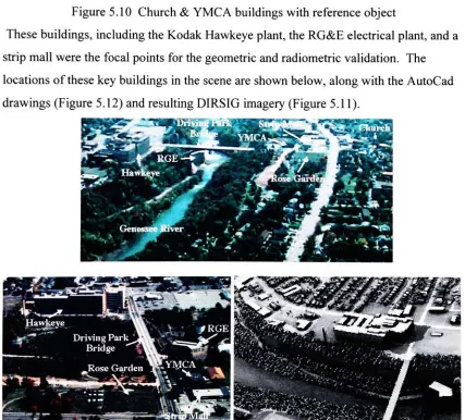
Figure 5.10

Church & YMCA

buildings

with

reference object

53

Figure 5.11

Scene

layout

53

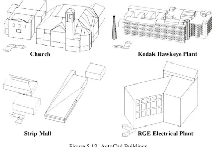
Figure 5.12

AutoCad Buildings

54

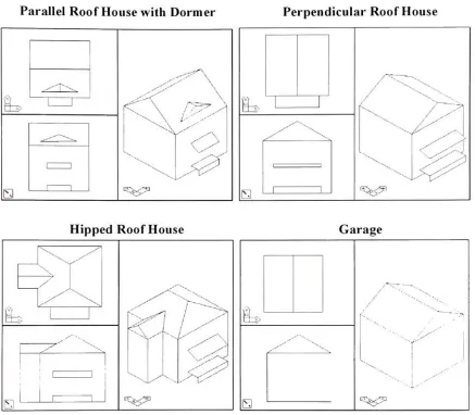
Figure 5.13

-

AutoCad Houses

55

Figure 5.14

Miscellaneous

object

details

56

Figure 5.15

Atmospheric

profile

57

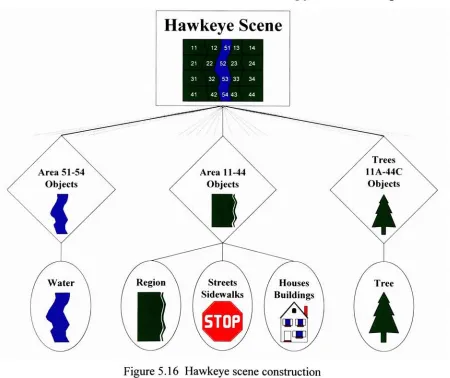
Figure 5.16

Hawkeye

scene construction

58

Figure 5.17

Primary

validation

imagery

66

Figure

5.18-

Validation

points

67

Figure 5.19

Material

evaluation

-temperature

comparison

69

Figure 5.20

-

Material

evaluation

ROC

results

72

Figure 5.21

Complex

phenomena validation points

74

Figure 5.22

Angular

effect evaluation

-asphalt streets

75

Figure 5.23

Angular

effect

&

shape

factor

evaluation

-asphalt shingles

77

Figure 5.24

Angular

effect curves

78

Figure 5.25

Angular,

shape

factor,

&

background

effect evaluation

grass

79

Figure 5.26

Angular,

shape

factor,

&

background

effect evaluation

- _r.g.

80

Figure 5.28

Ground

evaluation points

83

Figure 5.29

-Inframetrics

rank order correlation

imagery

85

Figure

5.30-

Inframetrics

rank order

correlation

results

86

Figure 6. 1

THERM

input

parameters

89

Figure 6.2

-

Shape factor

92

Figure 6.3

-

Material

orientations

96

Figure 6.4

-Meteorological

parameter

sensitivity

analysis

97

Figure 6.5

Material

parameter

sensitivity

analysis

flow

chart

104

Figure6.6

-

Material

parameter graph

analysis

105

Figure 6.7

-

Time

history

expected

temperature

error

analysis graphs

Ill

Figure 6.8

Time

history

sensitivity

analysis

-

Material

_comparison

113

Figure 6.9

DIRSIG

radiance

image

1 14

Figure 6.10

DIRSIG

debug

images

114

Figure 6.11

Angular emissivity

curve

115

Figure 6.12

-

Histogram

comparison

116

Figure6.13

-

Scene

analysis

118

Figure 6.14

-

Histogram

comparison

summary

126

Table 3.1

-

Radiance

equation

26

Table 3.2

Radiance

equation variable

definitions

27

Table 5. 1

Validation

imagery

-specification

summary

47

Table 5.2

Estimated

geometric

accuracy

60

Table 5.3

DIRSIG

input file

summary

60

Table 5.4

-

RMS

_{error validation}

results

Bendix

imagery

68

Table 5.5

-

ROC

validation

results

-

Bendix

imagery

72

Table 5.6

-^Angular

effect evaluation

-asphalt streets

76

Table 5.7

-

Angular

effect

&

shape

factor

evaluation

- _asphalt

shingles

77

Table 5

.

8

Angular, SF,

& background

effect evaluation

- _grass

&r.g

81

Table 5.9

-

Inframetrics ROC

results

86

Table 6. 1

Meteorological sensitivity

results

98

Table 6.2

Material

parameter

sensitivity

results

106

Table 6.3

-

Object

_{material parameter values}

124

Table 6.4

-

Input

1.0

Introduction

A

new

tank

with a

low

thermal

signature

has recently been designed

by

a

foreign

country.

Will

the tank

be detectable

by

existing heat seeking

missiles

or

does

a new

infrared

(IR)

sensor need

to

be designed

for

the

missile?-

Or

can

improvements

be

made

to

the

computer

algorithms

of

the

existing

missile

to

detect

the

new

tank?

While

it

would

be

difficult,

if

not

impossible,

to

determine

an answer

to these

questions

without

the

actual

use of

the

foreign

tank,

computer

models,

based

on

the

first

principles

of

physics,

can

actually be

used

to

answer

these

questions

before

the

military

forces

ever encounter

the

foreign

tank

in

a

real

world situation

when

lives may be

at risk.

With

the

increasing

capabilities

of

computers

in

the

last 20

years,

the

ability

to

model real world

situations,

such as

this

hypothetical

scenario

involving

a

low

thermal

signature

tank, has

dramatically

increased.

Specifically,

this

increase in computing

speed and

power

has led

to the

development

of

artificial

images

that

can

be

used

in

computer

animation,

flight

simulation,

and computer aided

design

and manufacturing.

This

process of

developing

artificial

images

is

known

as synthetic

image

generation

(SIG).

Synthetic

images

are

useful

in

a

vast

array

of

imaging

problems.

They

can

be

used

to train

analysts

on

the

appearance

of

a

target

under

different

meteorological

conditions,

times

of

day,

and

look

angles.

In

addition,

SIG

can

be

used

to

help

designers

evaluate various

sensor

systems

before

the

actual

hardware is

fabricated.

Synthetic

images

can also

help

determine

the

optimum acquisition parameters

for

a

real

imaging

system

by

predicting

the

time

at

which

the

greatest contrast

or

resolution

will

be

obtained

for

the

desired

targets.

The

result

is

a

large

savings

in

research and

development

cost

as

well

as

increased

performance and operational capabilities.

While

synthetic

images

can

be

created

in

virtually

any

regionof

the

electromagnetic

spectrum,

images

created

in

the

long

wave

(8-

14pm)

and mid

wave

(3

-5pm)

infrared

regions

offer unique signatures compared

to the

visible region.

Synthetic

images in

the

LWIR

and

MWIR

are

primarily

influenced

by

the

thermal

properties

and emissivities of

characteristics

and signatures

of

objects,

viewing

objects

in

simulated night

conditions,

and

finding

objects

hidden

or obscured

by

other

visible

features.

While

scale models

of

the

real world are often created

for

analysis of sensor

systems

in

the

visible

region,

it is

extremely

difficult

and often

impossible

to

build

miniature models

with

accurate

thermal

characteristics.

Thus,

synthetic

images

are one

of

the

only

ways

to

predict

the

performance

of

an

infrared

sensor system.

The

usefulness of

these

synthetic

images

is

negated

if

the

output

does

not

closely

imitate

the

real world.

As

a

result,

the

output

from SIG

must

be

evaluated and assessed

according

to

criteria

such

as

spectral and radiometric

accuracy,

geometric

fidelity,

robustness of

application,

and

speed

of

image

generation

(Rankin 1992).

Depending

upon

the

application and use

of

the

synthetic

image,

these

criteria will

have

differing

weights of

importance.

If

the

goal

of

the

SIG

process

is

to

produce

visually

appealing

pictures,

radiometric

fidelity

will

be

of

little importance

while speed of

image

generation

may be

favored.

However,

in

most

technical applications, the

speed

of

image

generation

is

sacrificed

for

radiometric

fidelity.

The

focus

of

this

project

is

validating

the

Digital

Imaging

and

Remote

Sensing

Image

Generation

(DIRSIG)

model

by

comparing DIRSIG

imagery

with real

airborne

imagery.

While DIRSIG

was validated

in

the

IR

region

in

1

992

by

Rankin,

several

modifications

have been

incorporated into DIRSIG

since

this

validation

(Schott

et.

al.,

1994). This

validation will

test

some of

these

modifications as

well as

the

robustness

of

DIRSIG

as

the

synthetic

images

are compared

to

infrared

imagery

taken

at

different times,

look

angles,

and

locations.

An

algorithm

for modifying

and

optimizing

the

object material parameters

was also

developed in

an attempt

to

reduce

the time

required

to

develop

accurate synthetic

images.

In validating DIRSIG

and

analyzing

the

input

parameters,

the

project

was

divided

into

smaller

tasks.

The

fist

step

was

to

define

the

exact goals and objectives of

the

were

researched

to

determine

the

weaknesses and strengths

of

DIRSIG. The

process

of

generating

a

DIRSIG

synthetic

image

was explained next.

All

this

background knowledge

led

to

a

technical

approach

that

could

be

used

in achieving

the

defined

objectives.

The

actual

experimental

validation of

DIRSIG

was

then

described

in

detail,

followed

by

the

sensitivity

analysis and optimization

of

the

input

parameters.

Recommendations for

2.0

Objectives

2.1

DmSIG Validation

While

DIRSIG

was validated

using

ground

truth

data in

the

IR

region

in 1992

by

Rankin,

synthetic

images

from DIRSIG have

never

been

extensively

compared

or

validated

with

actual aerial

imagery;

the

primary

validationprior

to this

work

used

roof

top

imaging

scenarios.

As

a

result,

the

validations

have

not

truly

explored

the

limitations

of

DIRSIG

and

its

ability

to

model

realaerial

imagery.

Rankin's

validation

focused

on

the

DIRSIG

submodels and

the

sensitivity

of

the

output

image

to

errors

in

various

input

parameters.

Each

ofthe

DIRSIG

subroutines

were

validated

individually

and recommendations

were

made

to

improve

the

synthetic

images.

These

recommendations

included

adding fractional specularity

and

transmissivity,

improving

the

shape

factor

computation,

adding

more materials

to the

material parameter

database,

modeling

clouds

in

the

scenes, and,

finally,

improving

the thermal

model.

Based

upon

these

recommendations, DIRSIG

has

been

modified

to

include fractional

specularity,

transmissive

objects,

and clouds.

However,

some of

the

other

options

have

not yet

been

implemented.

This

validation

concentrates

on

examining

DIRSIG'

s

current

ability

to

recreate

the

entire

imaging

chain,

from

end

to

end

(excluding

optical

and noise effects

-

DIRSIG has

these

capabilities

but

they

were not complete

at

the time

of

validation),

without

the

ability

to

examine each submodel

that

is

used

in

the

creation of

the

final

synthetic

image.

However,

it is

still possible

to

modify

the

input

parameters,

such

as

the

weather

file

and

material

file,

to

improve

the

radiometric

accuracy

of

the

final

synthetic

image. The

testing

also

differs from

the

previous

validation

in

that

it

further

explores

DIRSIG'

s

ability

to

include

atmospheric

attenuation

and

sensor geometric

effects

in

the

final

results.

Following

this

goal of

trying

to

evaluate

the

ability

of

DIRSIG

to

model

the

real

world,

several

images

taken

with

different

imaging

systems

and parameters will

be

used

in

the

validation.

The primary

comparison and

validationwill

be

accomplished

with

imagery

imagery

and

the

individual

material properties of all

the

facets

have

been

determined,

the

same scene

is

compared

to

the

secondary

truth

imagery.

The secondary

set

of

truth

imagery

from

an

Inframetrics

camera

greatly differs from

the

Bendix

truth

imagery.

The

Inframetrics

imagery,

which was acquired

at a

different

time

and

under

different

atmospheric

conditions,

will

help

test

the

robustness of

DIRSIG in modeling

imaging

conditions

of

the

same

target

scene.

In

conjunction

with

the

validationof

DIRSIG,

a

primary

objective

is

to

create a

complex and realistic scene

that

can

be

used

in future

studies and

testing.

Synthetic

imagery

provides a

useful

tool

to

test

image

algorithms and

analysis

techniques, but it

must

closely

resemble

the

real world.

The

scene

that

is developed for

the

validation will

provide

this

capability.

It

will

bridge

the

gap between

the

past validation of

DIRSIG,

where a

simple scene

with

known

test targets

was

used,

and real

imagery,

where

little

actual

information is known. In

order

to

make

the

scene

as realistic as

possible,

the

scene

must contain

the

complex

interactions

between

objects,

including

buildings, houses,

trees,

and

other

structures

that

are

found

in

the

real world.

This

requires extensive

research of

the

objects

in

the

scene

so

that

they

can

be

recreated accurately.

The

research and effort

in

building

the

scene

was

shared

with

Russell White

who will validate

DIRSIG in

the

2.2 Input

Parameter

Analysis

& Optimization

In

addition

to

validating

DIRSIG,

a

procedure

for

optimizing the

synthetic

image

input

parameters

was

developed.

Previously,

a

trial

and

errorprocess

was

used

to

modify

the

input

parameters

until

the

synthetic

image closely

resembled

the truth

imagery.

A

better

method

for

determining

these

input

parameters

is

needed

to

reduce

the time

required

to

generate

an

accurate

synthetic

image. This is

accomplished

by

first

determining

the

bounds

or

limiting

values

for

each of

the

input

parameters,

and

then

determining

the

effect

of each

input

on

the

synthetic

image. This step

alone

is

an

improvement

over

the trial

and

error

guessing

process

that

was

previously

used.

While

bounding

values are

helpful in

determining

the

range of values

for

the

input

parameters,

the

most

effective

way

to

fine

tune the

input

parameters

requires

a

sensitivity

analysis

of all

the

parameters.

A sensitivity

analysis shows which parameters

create

the

largest

changes,

and

therefore,

most probable

error

in

the

synthetic output

image. The

parameter with

the

highest sensitivity

can

then

be

altered

first

to

try

and

match

the

synthetic and

real

imagery,

or

a

combination of

the

most sensitive

parameters

can

be

altered

to

create

the

desired

output.

In

addition,

a confidence

interval

in

the

estimation

of

the

input

parameters,

i.e.

an estimated

error,

should

be developed for

each

input.

Similar

to the

sensitivity

analysis,

this

will

indicate

which

parameters are most

likely

to

cause

error

in

the

output

image.

The sensitivity

analysis and

the

error estimation will

provide

tools

for

the

input

parameter optimization

process.

For

example,

a

large

error

in

the

estimation of a

material

parameter can

be

tolerated

if

the

output

image

is

not

sensitive

to

variations

in

that

variable;

however,

it

would

be

essential

to

alter

a

parameter

with

a

large

error

in its

predicted value

if

the

image is

highly

sensitive

to

that

parameter.

This

method

of

fine

tuning

the

material parameters

will

likely

reduce

the time to

generate

synthetic

images

while

also

establishing

guidelines

for

eventually

automating

the

selection

and

modification

ofthe

material

parameters.

Images

of

the

same

region of

interest

acquired

under

different

imaging

conditions,

such

as a

nadir versus

oblique

look

angle,

or

morning

versus night

acquisition,

are also

exact same appearance

under

different

imaging

conditions.

The

multiple

images

of

the

same scene

may

provide

insight into

the

reflectivity

and

emissivity

of

the

objects

in

the

scene.

For example,

the

temperature

of an aluminum-sided

building

and

a wood-sided

building

that

have

been

wanned

by

direct

sunlight

will

be

vastly

different

when

compared

to the

respective

temperatures

on

a

cloudy day.

On

a

sunny

day,

the temperature

of

the

aluminum rises

rapidly

as

the

energy from

the

sun

is

absorbed,

but

on

the

cloudy

day,

the

temperature

of

the

aluminum

will

not rise

as

much.

Similarly,

the

temperature

of

a

wood-sided

building

will

be

greater on

a

sunny

day

than

on

a

cloudy day.

However,

the

wood-sided

building

will

not

have

a

large

change

in

temperature

between

the

cloudy

day

and

the

sunny

day

because

wood

has different

thermal

properties

than

aluminum.

It

is

the

difference

in

appearances

of

the

objects

that

can

help

indicate

some of

the thermal

material

properties.

The

facet

material parameters can

then

be

adjusted

to

logically

account

for

the

images

generated

under

the

different

acquisition parameters.

The

use

of multiple

images

3.0

Background

3.1 The

Big

Equation

In

order

to

understand

the

synthetic

image

generation

process,

it is first

necessary

to

understand

the

physics and

underlying

principles

that

are

involved

in

the

capture

of

a

real

image.

The

first

step

is

to

visualize

how

the

observed

electromagnetic

radiation

ultimately

reaches

the

sensor.

The

observed

radiance at

the

front

end of

the

sensor

is

comprised

of

nine

different

photon paths.

The

following

diagrams

show

the

different

paths

that

electromagnetic

radiation

may

travel

before reaching

the

sensor.

The

first

diagram

shows

the

radiation

originating from

solar

photons while

the

second

diagram

shows

the

radiation

resulting from

self-emission

by

the

objects.

Figure 3

.

1

Solar energy

photon paths

Type A

-Directly

reflected solar photons attenuated

by

the

atmosphere and clouds

Type B

-

Solar

Photons

reflected

from

the

background

onto

the target

Type

C

-

Solar

photons scattered

by

the

atmosphere

Type

G

-

Solar

photons scattered

by

the

atmosphere onto

the target

solar "-photons ^-photons '&photons '

^

photons

=

E"

cosa'-r^

+

F-Edsl

-r2

+(\-

F)-LbsXrdz2

+

Lu

Figure 3.2

-Self-emitted energy

photon paths

Type D

-

Self-emitted

photons

from

the target

attenuated

by

the

atmosphere

Type

E

Self-emitted

photons

from

the

sky

reflected

by

the target

to the

sensor

Type

F

-

Self-emitted

_photons

from

the

atmosphere

Type H

Self-emitted

photons

from

the

background

reflected

by

the

target to the

sensor

t

=

D

₊

F

₊

F

₊

H

self-emission photons photons photons photons

=

Ltx

^2+F-EdeXr2+(\-

F)rd LbeX

t2

+

LueX

n

(3.2)

After combining

these two

equations,

Za

=

Lsoiar+Lseif.em,ssw^

the total

spectral

radiance

reaching

the

sensor

can

be

described

by

the

following "big

equation":

r{X)

rM)

Lx

=Escosa'^^z](X)T2(l)

+

(A)LTXT2(X)

+

F[Edsl+EdX]^-^-T2(A)

+

K K

{\-F)[LbsX+Lbxyd(A)z2(A)

+

LusX+Lu

cX

(3.3)

Es

Exoatmospheric

irradiance

cos a

-the

angle

from

the

target

normal

to

the

sun

zi

-

transmission

of

the

atmosphere

from

the

sun

to

the

target

t2

-

transmission

of

the

atmosphere

from

the target

to the

sensor

e(X)

-target

emissivity

Itx

-

self-emitted radiance

from

target

at

temperature

T

Edsx

-solar

downwelled

irradiance

Edex

-

self-emitted

downwelled irradiance from

the

F

-shape

factor

(amount

of

sky hemisphere

that

the

target

can

see)

1-F

-the

percentage of

the

atmosphere

that

is

blocked

by

the

background

object

rd(X)

-

target

reflectance

Ibsx

-

background

_radiance

from scattering

Lbcx

-

background

radiance

from

self emission

LuSa

-upwelled

radiance

due

to

scattering

of

the

atmosphere

LUEx

-upwelled

radiance

due

to

the

self emission

of

the

atmosphere

This

equation represents

all

the

sources

of radiation

that

are

of

significant

importance

in

determining

the

radiance

that

reaches

imaging

systems sensitive

to

0.3

-14.5u.rn

wavelengths.

As

noted,

this

equation

is

dependent

upon

the

wavelength.

Depending

upon

the

spectral

sensitivity

of

the

imaging

system,

this

equation

may be

simplified

by

neglecting

certain

terms

since

their

effects are

minimal

at

those

wavelengths.

While

both

solar photons

and self-emissive

photons must

be

accounted

for in

the

MVVTR,

solar

photons are

of

little

importance

for

this

validation and can

be

neglected

in

the

3.2

Alternative SIG

Models

In

order

to

generate

any

synthetic

image,

several

inputs

must

be defined

to

produce

the

desired

objects

in

a specified

environment.

For

almost

all computer

models,

these

basic

inputs include

a geometrical

representation of

the

object,

an atmospheric

transmission

model,

radiation sources and

material characteristics.

Some

models

also

include

texturing

abilities and

thermal

submodels.

The

overall

accuracy

of

the

final

synthetic

image depends

on

the

individual

accuracy

and

integration

of

these

submodels

as well

as

the

intended

use of

the

synthetic

images.

Therefore,

it is

beneficial

to

examine other

SIG

models

to

learn

where

improvements

might

be

made

to

the

current

DIRSIG

program.

One

ofthe

leading

computer

models

for

the

creation of accurate

radiometric synthetic

images

was

developed

by

the

Electromagnetics

Laboratory

of

the

Georgia Tech Research

Institute

(Cathcart

and

Sheffer,

1988

a,

1988

b)

This

SIG

program, the

Georgia Tech

Visible

and

Infrared Synthetic

Imagery

Testbed

(GTVISIT),

integrates

the

outputs

from

the

submodels

MAX, GTSIG, IRMA

and

MODELIR

to

create

a

synthetic

image. Each

GTVISIT

scene

is

comprised of

two

main

aspects,

a gridded

terrain

background

and

faceted

objects

located in

that

background.

The

gridded

database

consists

of

features (material

types),

elevations,

radiance

values,

and

thermal

IR

reflectances

where

the

elevation and

feature

data may

be

real, synthetic,

or

a

hybrid,

and

the

radiance

and

infrared data

are

determined

from

the

temperature

and

reflectivity

of

the

object.

The

following

diagram

outlines

the

inputs

and

process

in creating

a

GTVISIT

synthetic scene.

OBJECTS

Geometric

Model

Radiance

Model

Sensor

Path

Locations

GTVISIT

Background

Radiance

Gridded

Database

Topographical

Data

Using

all

the

various

inputs into

GTVISIT,

it is

then

necessary

to

integrate

these

parts and

determine

the total

radiance

reaching

the

sensor.

Different

models propagate

the

radiance

from

the

scene

to

the

sensor

through

several

techniques.

While DIRSIG

employs

a

ray-tracing

method,

GTVISIT

uses

a

Z-buffer

algorithm

based

on

the

principle

of

displaying

or

concealing

surfaces

using

a

visual

line

of sight

to the

sensor.

GTVISIT

also

includes

atmospheric

attenuation

for

each object

in

the

scene

by

pre-computing

the

radiance values

in 12

orientations and

then

assigning

an atmospheric radiance value

to the

facet. The

thermal

radiance

values

are

then

computed

using first-principles

techniques

contained

in

the

GTSIG

submodel of

GTVISIT.

By

modeling

all

these

real world

phenomena,

GTVISIT

creates

fairly

realistic

radiometric

images.

However,

it falls

short

in

that

it does

not

account

for

angular

emissivities

or

background

effects

on

the

radiance of

the target.

In

addition,

GTVISIT

does

not

determine

the

solar

history

for

the

objects

in

the

scene.

Thus,

while

GTVISIT

is

one

of

the

leading

developers

of radiometric synthetic

images,

there

is

still room

for

improvement.

The Physical Reasonable Infrared

Signature

Model,

PRISM,

is

an

extremely

detailed

model

relying

on

highly

sophisticated

CAD drawings

to

create

radiometrically

accurate

models

of

vehicles,

primarily

tanks

(Gonda

and

Gerhart,

1989).

This

modelrelies on

3-D

isothermal

facets

that

interact

witheach other

through

conduction, convection,

and

radiation.

PRISM

models

both

the

internal

and

external

features

of

the tank.

Using

a

Faceted Region Editor

(FRED),

BRL-CAD

vehicle

descriptions

are

translated

into

a

format

that

PRISM

can

then

use

to

predict

the thermal

signature.

PRISM

is

also

able

to

calculate

the

solar

history

and

hence

temperature

of each

facet

for

a

diurnal

time

period.

However,

PRISM

fails

to

calculate

the

interactions between

the

target

and

the

background.

Targets

are

"cut

and

pasted"

into background

scenes.

PRISM

creates

very

realistic

images,

but

the

difficulty

in creating

the

detailed drawings

and

its

failure

to

account

for

the

interactions between

the

background

and

the

target

prevent

its

widespread

Texas

Instruments

(Tl)

has

also

developed

a

synthetic

image

generator

for

use with

automatic

target

recognition

(ATR)

algorithms

(Lindahl

et

al.,

1990). This

multi-sensor

synthetic

image

generator

is

capable of

producing

IR,

television

(TV),

and

Laser Radar

images.

The

following

diagram

illustrates

the

Tl

synthetic

image

generation process.

Sensor

Information

Terrain

Map

All Objects.

Scene

Geometry

FOVAREA

DETERMINATION

Active Terrain Object clipping Information

OBJECT

FOV CLIP

Active Objects

TERRAIN

AND

OBJECT

TRANSFORMATIONS

Ground

Truth

Information

Scene

Shading

SUN TO

SURFACE

VISIBILITY

TransformedPoints

VISIBLE

SURFACE

DETERMINATION

Normal " Vectors " Resolution Information

High Resolution

Geometry Array

Ground Truth

(GT)

Information

GREYSHADE

APPLICATION

ANTI

ALIASING

High Resolution Shaded Image

->GT Info

-?Sensor Resolution Shaded Image Point Greyshades Edge List

Figure 3.4 Tl

synthetic scene generation

(Lindahl

et

al.,

1990)

Similar

to

most

SIG's,

Tl

uses

faceted

objects placed

in

a

fractal interpolated

background

environment

derived from Defense

Mapping Agency (DMA)

Digital Terrain Elevation

Data

(DTED)

and

Digital Feature Analysis Data

(DFAD).

The

objects,

which

are created

using AutoCad

10,

are

initially

placed onto

the terrain

scene

using

world

coordinates and

then

both

the terrain

and

the

objects are

translated to

sensor coordinates.

Trees may

also

be

added

to the

scene

using

a

fractal

initiator/generator

technique.

Similar

to

GTVISIT,

a

Z-buffering

algorithm

is

then

used

to

determine

which

objects are

hidden from

the

sensor

by

other surfaces.

LOWTRAN 7

is

also used

to

predict atmospheric

transmission

and

attenuation.

The Texas

Instruments

synthetic

image

generator also

includes

the

ability

to

include

sensor effects

for

each of

the

different

sensor

types;

colored-noise

that

resembles

to

speed

the

generation

of

the

synthetic

image,

"a

two-dimensional

Gaussian

point-spread

function is

used

to

approximate

the

effects

of optical

diffraction

and

blur,

detector

and

LED

spatial

response,

and

stabilization

jitter for both

the

IR

and

TV

sensors"

(Lindahl

et

al.,

1990).

TFs

multisensor synthetic

image

generator sacrifices radiometric

accuracy for

computational speed.

Its

use of

gray-shading

and exclusion of solar or specular

effects

in

the

synthetic

images

reduce

its

abilities

to

model

the

real world.

The

results are

realistic

looking

images,

but have

questionable

radiometric

fidelity.

It

provides useful

synthetic

images for

automatic

target

recognitionalgorithms which

rely

more on

relative

image

contrasts

than

absolute radiometric accuracy.

Therefore,

while

this

systemcan model

many

different

sensors,

it is

of

little benefit

to those

trying

to

assess

the

absolute

radiometry.

Aerodyne

Research,

Inc.,

currently

uses

the

SPIRITS 2.0 (Spectral Infrared

Imaging

of

Targets

and

Scenes)

infrared SIG

program

for modeling

aircraft

targets

and

exhaust

plumes

(Stets

et

al.,

1988).

Relying

on

the

LOWTRAN

atmospheric model and

IR

Cloud

Radiance Model

(CLOUD)

to

recreate

the

atmosphere,

SPIRITS

integrates

the

results of

cluttered

background

of

terrain,

sky

and cloud

with

target

images. While

this

program produces

very detailed

results

of

aircraft and

vehicles with

exhaust

signatures,

it has

some

limitations.

It

fails

to

create

high

resolution

ground scenes and

even

treats the

earth

as a

flat

object

with

a

uniform

temperature

and

diffuse

reflectivity.

In

addition,

because

the

target

and

background

are computed

separately,

it

is

not

possible

to

include background

effects

in

the

calculations;

however,

this

does

not

greatly detract from

their

model

since

most

of

their

scenes

involve high

flying

aircraft.

This

approach

would

not

be

possible

for

use

by

DIRSIG

when

high

resolution

ground scenes

with radiometric

accuracy

are

the

primary

goal.

A

new version

of

this

program

known

as

AC-1

is

scheduled

for

release

next

year.

Some preliminary information

about

this

new program

will

be

available

soon

for

The

Simulated

Infrared Image

(SIRTM)

program created

by

the

Environmental

Research

Institute

of

Michigan

(ERTM)

is

vastly different from

other

thermal

synthetic

models.

It

calculates

temperatures

based

on

the

3-D

volume

of

an

object,

versus

traditional

surface

modeling.

The

volume

modeling is

achieved

by

subdividing

the

volume

of

an object

into

elements

call voxels.

"The

voxels are

simply

cubic solids

that

fill

the

volume

of

the

object"

(Lyons

1991).

This division

of

the

object

into

voxels

allows

for

complex

thermal

interactions

and results

in

accurate

temperature

predictions.

Thus,

it

could

be

useful

in modeling

thermal

plumes and othervolumetric shapes

that

have

complex

thermal

gradients.

Because

of

this

unique

modeling

of

object

volumes,

the

geometric representation

of an

object

is defined using

constructive solid

geometry

(CSG)

models

in BRL-CAD.

Boundary

model

representations,

including

wireframe

and surface

models,

may be

converted

to

CSG

models

using

specialized

translation

programs.

Similar

to

other

high

end

thermal

SIG

models,

a

ray

tracer

is

also

used.

The

ray-tracer

aids

in

creating

the

voxels,

determining

the

solar

loading

of

the voxels,

and

accounting for

target-background interactions.

Four primary

modules are used

in

the

image

generation

process,

in

addition

to the

geometric

modeling

and

ray-tracing.

The information first

travels

into

the

VOXCRE

module where

the

object

volume

is divided into

voxels.

The information

is

then

directed

to the

VOXSUN, SVOXTMP,

and

RADCLC

modules.

The VOXSUN

module,

in

conjunction with

the

ray-tracer,

determines

which voxels are exposed

to

solar

heating

and

outputs

the

results

to the temperature

prediction

module,

SVOXTMP

SVOXTMP

accounts

for

the

conduction,

convection,

and

radiation exchange

between

the

voxels and

surrounding

object

voxels

as

well

as

the

environment.

The

output

is

a

"three-dimensional

temperature

distribution

of

the

object as a

function

of

time

but independent

of sensor or

viewing

geometry."

The

temperature

results are

then

used

in

the

RADCLC

module

to

determine

the total

radiance.

The RADCLC

module

integrates

the

self

emission

of

the

object

due

to temperature

and

the

reflected

radiance

from

the

environment.

This

is

where

SIRIM does

not propagate

this

radiance

to

a

sensor or

include

any

atmospheric

transmission effects;

it is

not a complete end-to-end

simulation

package.

This

is

a

major

limitation

of

SIRIM.

In

addition,

the time

required

for

the temperature

calculations are

extremely

time

consuming

and

computer resource

intensive.

If

speed

improvements

could

be

made

to the thermal calculations,

SIRIM

would

be

a valuable

replacement

to

THERM,

the

DIRSIG

thermal

model.

In

its

current

form,

the

prolonged run

times

of

SIRIM

weighed against

the

added

thermal

accuracy do

no

warrant

its integration

into

DIRSIG.

By

examining

other

synthetic

image

generation

programs,

it is

possible

to

determine

the

strengths and

the

weaknesses

of

these

other

SIG

models.

The ideal

solution

would

be

to

create a synthetic

image

generation

program

that

incorporated

the

strengths of all

the

3.3

DHISIG Overview

In

order

for

a synthetic

image

to

accurately

resemble

the

real

world,

it

is necessary

to

develop

a

complete

mathematical model of

the

entire

imaging

chain.

This

requires

an

understanding

of

the thermal

radiance

of

the

objects

in

the

scene as

well

as

the

atmospheric

effects

on

the

radiance

that ultimately

reaches

the

IR

sensor.

The

sensor

effects must also

be

incorporated into

the

model

to

create

realistic synthetic

images.

With

all

these

inputs,

it is

then

possible

to

try

and

develop

a

synthetic

image.

DIRSIG

attempts

to

model

the

entire

imaging

chain

using

the

inputs from

various

submodels.

The

following

diagram,

Figure

3.5,

provides

a

brief

overviewof

the

submodels used

in recreating

the

Ltreal

world"

for

a

DIRSIG

synthetic

image.

Each

of

these

submodels

will

be described in

detail.

Geometry

Sensor

Submodel

I

Submodel

Ray-Tracer

Submodel

Final

Image

I

1

Thermal

Submodel

Radic

Sub

>metry

model

Figure

3.5 DIRSIG

overview

3.3.1

Scene

Geometry

Submodel

In creating

a

synthetic

image,

one

of

the

first

steps

is

to

build

geometric models

of

the

3

-Dimensional

objects

that

will

be in

the

output

image.

This

is

accomplished

using

computer

aided

design

software

known

as

AutoCad

that

has been

enhanced

with specialized

DIRSIG

related routines.

In

order

to

develop

a scene

that

can

be

used

by

DIRSIG,

it is

necessary

to

create parts and objects

that

are made

up

of

individual facets.

A

facet is

a

collection of

points,

usually

triangular

or

rectangular,

with

a

normal vector

that

describes

the

convex

plane.

These

facets

are

the

elementary

building

blocks

to

which

various

parameters or attributes are assigned and are

then

be

used

by

the

other

DIRSIG

Attributes

Material Name

Material

Code

-yto;-;--N

Default

Temperature Thickness

Self-Generated Power

Default

Shape Factor

Material Properties

Figure

3.6

Facet

material parameters

The

faceted

parts

are

then

combined

to

form

an

object,

and,

finally,

multiple objects

may

be

integrated into

one

drawing

to

create

the

final 3-D

scene,

as

depicted in Figure 3.7.

Scene

Node

Figure

3.7

DIRSIG Data

Hierarchy

(Schott

et

al.,

1993)

A

certain

data

structure

and

hierarchy

of

information is

assigned

to the

each

object,

computations

and require more

computer

storage

memory.

Starting

at

the

highest

level,

the

scene node contains

the

name,

date,

geographical

coordinates,

and

number

of objects

of

the

scene.

The

object node

then

contains

the

name,

ID

number,

number of

parts

in

that

particular object

with

pointers

to

nodes

describing

each

part,

and

the

coordinates

that

define

the

edges

of

the

bounding

volume.

The

bounding

volume of

the

object

is

used

when

the

rays are cast

into

the

scene

(see Figure 3.8). If

the

ray does

not

hit

the

bounding

region of

the object,

it

is

not

necessary

to

cast

the

ray into

the

parts

and

facets

of

that

object.

This

helps

to

reduce

the

computation

time

for

the

ray-tracer

submodel.

The

part

node

data

structure

is

the

same

as

the

object

node,

with

bounding

volumes

to

eliminate

the

need

to

check each

facet

within

the

part

for

a

ray intersection.

Finally,

the

facet

node

links

the

geometric

location

and orientation

of

the

facet

with

the

material properties.

/

/

"

l-r-O-ft

/

^^^

^

volume

/

\

^aAifioW-^

/

\

__

facet

^+@-^fnr(

object

bounding

volume

Figure

3.8

Object &

part

bounding

volumes

(Schott

et

al.,

1993)

After

all

the

DIRSIG

hierarchy

has been

established

and

the

scene

is

complete,

the

AutoCad

scene

is

then

'translated'

into

real world geographical coordinates so

that

the

other

submodels

of

DIRSIG

can

recognize

the

inputs.

3.3.2

Ray-Tracer Submodel

The

ray-tracer submodel

is

the

vital

connection and

link

to

all

the

DIRSIG

submodels.

This

submodel

retraces

the

hypothetical

path of a

photon after

it

has

reached

the

sensor.

Beginning

at

an

individual

pixel

in

the

synthetic

image,

a

ray

is

cast

into

the

Sensor

Field oi viewin Y

Fieldof viewinX

Mpixels

Figure

3.9 Ray-tracer

(Schott

et

al.,

1993)

An

iterative

process

is

used

to

determine

the

interaction

of

the

ray

with each

object, part,

and

facet

in

the

scene.

From

these

interactions,

the

path of

the

radiance

reaching

the

sensor can

be

determined.

The energy

losses

and gains

associated

with

the

atmosphere

are

included

in

the

process.

This

allows

the

proper radiance at each pixel

to

be

computed

by

the

radiometry

submodel.

The radiometry

submodel

is

described in detail

in

Section 3.3.4.

Because

each

ray

must

be

tested

for intersection

with

every

single

object

in

the

scene,

bounding

volumes

for

each object and part were

developed

to

reduce

the

numberof

interactions

that

must

be

examined.

This

process reduces computation

time

because

if

an object

is

not

hit

by

the ray,

it

is

not

necessary

to

determine

the

interaction

of

that

ray

with

the

sub-parts or

facets.

These

bounding

volumes

may

be

parallelepipeds, cubes,

or spheres.

If

a

ray

hits

a

particular

object,

it is

then

checked

with

the

parts

in

that object,

and

finally,

the

interaction

with

the

individual facets is

determined. If it

is

found

that

a

facet has been

hit

by

a

ray,

the

solar

history

of

the

facet is

established so

that

a

more

accurate

temperature

can

be

predicted

by

THERM. THERM

uses

direct

insolation,

or

direct

sunlight

values,

from

the

weather

file

to

more

precisely

predict

the temperature

of

The

solar

history

of

the

object

is

stored

in

an

array

as a

function

of

time

with values

ranging

from

0

to 1

.

|0.0|1.0|1.0|02|0.1|0.0|0.0|0.0|0.0|0.0|1.0|1 0|10|1.0] 0 1 2 3 4 5 6 7 8 9 10 11 12 13

Figure 3.10 Solar

history

(Schott

et

al.,

1993)

If

the

object

was

illuminated

by

the

sun

at a

particular

time,

a

value greater

than

0

is

placed

in

the

array

and

the

solar

loading

term

in

the

weather

file is

weighted

by

this

value.

However,

if

the

object

has

been

in

the

shadow or not

illuminated

by

the

sun,

a

value of

0

is

placed

into

the

array.

Therefore,

when

the

solar

loading

value

in

the

input

weather

file

is

multiplied

by

the

solar

history

value

of

0,

the

overall effect

is

a zero solar

loading

term

when

the target

has

been in

shadow.

After

the

solar

history

of

the

facet has been

determined

and

the

resulting direct insolation

values

have been

calculated,

the temperature

of

the

facet may

then

be

computed

by

THERM.

Once

a

ray hits

a

facet

and

the

solar

history

has been

calculated,

the

interaction

between

the

ray

and

the

facet depends

on

the

specularity

and shape

factor

of

the target

A

target

may be

specular,

diffuse,

a

combination of

the

two,

or even

transmissive

(see

Figure

3.11). The

shape

factor

of

the

facet is

also calculated at

this time

as

additional

rays

are cast

from

the

facet

to

determine

the

amount

of atmosphere

that

is

blocked

by

surrounding

objects.

Totally

Specular

Totally

Diffuse Combination of Specular & Diffuse

Transmissive

If

the

facet

is

reflective,

then

secondary

rays must

be

cast

out,

similar

to the

original

ray-tracing

method.

For

completely

specular

targets,

a single

ray

is

cast out at an angle equal

to the

incidence

angle.

The

properties

of

the

background

are

determined

and

then

used

to

calculate

the

radiance

ofthe

target

facet.

However,

most

targets

are

not

completely

specular.

This

requires

a

more rigorous

method of

determining

the

background

effects.

Therefore,

'diffuse'

secondary

rays are cast out

over

the

hemisphere

at

15

increments

in

the

zenith and

30

increments

in

the

azimuth.

The

procedure

for

determining

the

background

hits

is

the

same as

for

the

specular case:

test

each

object, part,

and

facet.

Then,

for

each

secondary ray

that

is

cast,

the temperature

and properties of

the

object

that

is

hit

are recorded.

The

combined effects

of

these

secondary

hits

are

integrated

to

approximate

the

diffuse

radiance value

reaching

the target.

While

this

process

of

casting

rays could continue

indefinitely,

a

maximum

of

two

bounces i