Statistical analysis of coverage error in simple global temperature estimators

This is a repository copy of

Statistical analysis of coverage error in simple global

temperature estimators

.

White Rose Research Online URL for this paper:

http://eprints.whiterose.ac.uk/134340/

Version: Published Version

Article:

Cowtan, Kevin Douglas orcid.org/0000-0002-0189-1437, Jacobs, Peter, Thorne, Peter et

al. (1 more author) (2018) Statistical analysis of coverage error in simple global

temperature estimators. Dynamics and Statistics of the Climate System: An

Interdisciplinary Journal. ISSN 2059-6987

https://doi.org/10.1093/climsys/dzy003

Reuse

This article is distributed under the terms of the Creative Commons Attribution (CC BY) licence. This licence allows you to distribute, remix, tweak, and build upon the work, even commercially, as long as you credit the authors for the original work. More information and the full terms of the licence here:

https://creativecommons.org/licenses/

Takedown

If you consider content in White Rose Research Online to be in breach of UK law, please notify us by

Statistical analysis of coverage error in simple

global temperature estimators

Kevin Cowtan

, Peter Jacobs

, Peter Thorne

, Richard Wilkinson

a

Department of Chemistry, University of York. York, UK.

[email protected]

b

Department of Environmental Science and Policy, George Mason

University, Fairfax, VA, USA.

c

ICARUS, Maynooth University, Maynooth, Ireland

d

School of Maths and Statistics, University of Sheffield, Sheffield,

UK

Abstract

Global mean surface temperature is widely used in the climate literature as a measure of the impact of human activity on the climate system. While the concept of a spatial average is simple, the estimation of that average from spa-tially incomplete data is not. Correlation between nearby map grid cells means that missing data cannot simply be ignored. Estimators that (often implicitly) assume uncorrelated observations can be biased when naively applied to the observed data, and in particular, the commonly used area weighted average is a biased estimator under these circumstances. Some surface temperature prod-ucts use different forms of infilling or imputation to estimate temperatures for regions distant from the nearest observation, however the impacts of such meth-ods on estimation of the global mean are not necessarily obvious or themselves unbiased.

This issue was addressed in the 1970s by Ruvim Kagan, however his method has not been widely adopted, possibly due to its complexity and dependence on subjective choices in estimating the dependence between geographically proxi-mate observations. This work presents a simplification of that estimator based on generalized least squares which is fully specified by two equations and a single parameter, and can be implemented in fewer than 20 lines of computer code. The performance of the estimator is evaluated using reanalysis data with artificial noise, and for recent years mitigates most of the error associated with the use of a naive area weighted average.

These improvements arise from the fact that coverage bias in the historical temperature record does not arise from an absolute shortage of observations

(at least for recent decades), but rather from spatial heterogeneity in the dis-tribution of observations with some regions being relatively undersampled and others oversampled. The new estimator addresses this problem by reducing the weight of the oversampled regions, in contrast to some existing global tempera-ture datasets which extrapolate temperatempera-tures into the unobserved regions. The results are almost identical to the use of kriging (Gaussian process interpola-tion) to impute missing data to global coverage, followed by an area weighted average of the resulting field. However, the new formulation allows direct diag-nosis of the contribution of individual observations and sources of error. More sophisticated solutions to the problem of missing data in global temperature estimation already exist, however the simple estimator presented here and the error analysis that it enables demonstrate why such solutions are necessary.

The 2013 Fifth Assessment Report of the Intergovernmental Panel on Cli-mate Change discussed a slowdown in warming for the period 1998-2012, quot-ing the trend in the HadCRUT4 historical temperature dataset from the United Kingdom Meteorological Office in collaboration with the Climatic Research Unit of the University of East Anglia, along with other records. Use of the new es-timator for global mean surface temperature would have reduced the apparent slowdown in warming of the early 21st century by one third in the spatially incomplete HadCRUT4 product.

1

Introduction

Global mean surface temperature change is a key metric in the quantification of global warming (Stocker et al., 2013). Surface air temperature is significantly influenced by local and seasonal factors, such as altitude, exposure and surface type, so the metric is usually expressed in the form of a global mean surface temperature anomaly, which is the areal average of the temperature deviation from an average over some reference period of the temperatures for that location and month of the year (Jones et al., 1999). The global mean surface temperature anomaly is then defined as the areal average of these local temperature anomalies over the whole of the surface of the planet (Equation 1) whereTgl is the global

mean surface temperature anomaly for a given month, T(λ, φ) is the anomaly at a given latitudeλand longitudeφ, andA is the area element.

Tgl =

RR

T(λ, φ)dA RR

dA (1)

representative of the average temperature in the region spanned by the grid cell). The global mean is given by Equation 2, where Ti is the temperature in a given grid cell andai is the area of the grid cell denoted by the index i:

Tgl≈

P iaiTi P

iai

=w⊤_glT (2)

wherewgl is the vector of normalized weightsai/Piai andTis the vector of

temperaturesTi.

However, observational data typically do not have global coverage, i.e. there are grid cells for which the measurements are missing. In the simple case where all the grid cells are uncorrelated, we could view the partial coverage as a random sample from a population. Then the best estimator of the global mean would be the sample mean (i.e. the mean of the available grid cells weighted by the cell areas), and this will be an unbiased estimator of the global mean surface temperature anomaly.

In practice the observations (or more strictly the deviations from the global mean) are spatially correlated Vinnikov et al. (1990), which complicates mat-ters. It is useful here to introduce terminology from the statistics literature (Graham, 2009; Little and Rubin, 2002), where a distinction is made between data that are missing completely at random (MCAR), missing at random (MAR), and missing not at random (MNAR). Missing data are MCAR if the missingness mechanism is independent of other information, in our case, if the probability a grid cell record is missing does not depend upon a cell’s location or the tem-perature anomaly. The data are MAR if the missingness depends upon the covariates, but not the quantity of interest, i.e., the probability a cell record is missing can depend upon its latitude and longitude but not the tempera-ture anomaly. MNAR data occur when the missing mechanism depends on the quantity of interest, for example, if a temperature observation was censored for being too high or low. Only MCAR data can be analysed using complete data techniques by simply ignoring the missing values. In particular, the use of the sample mean as an estimator for the global mean is contingent on the assump-tions of ordinary least squares, namely that observaassump-tions are a random sample from the population and that the errors are uncorrelated, or in other words that the missing data are MCAR. When applied to MAR and MNAR data, the sam-ple mean can lead to biased estimates. For the temperature data, missingness is strongly correlated with longitude and latitude, with, for example, data at high latitudes more likely to be missing. The observations are therefore at best miss-ingconditionally at random (MAR), so that unless we control for the influence of longitude and latitude statistical estimators based on the data will be biased. The observations could also be missing not at random (MNAR) due to manual station selection or outlier rejection, however, the resulting biases would not be detectable or correctable without reference to a larger set of weather station data such as that of Rohde et al. (2013) or Rennie et al. (2014).

Uni-versity of East Anglia (Morice et al., 2012) and the weather station contribu-tion to the Japan Meteorological Agency record (Japan Meterological Agency, 2017), however in both cases the global mean is determined from the mean of the grid cells for which values are available (with an additional step to equal-ize the weight of the hemispheres in the case of Morice et al.). More sophis-ticated methods developed for dealing with missing temperature data assume a MAR mechanism, and then try to compensate for the missing data either by using a more sophisticated estimator for the global mean, or by imput-ing the missimput-ing data before usimput-ing complete data techniques. For example, the variance-covariance matrix of observations is used directly in the opti-mal estimation of global mean surface temperature by Kagan (1979), Kagan (1997), and has also been employed by Vinnikov et al. (1990), Gandin (1993), Smith et al. (1994) and Weber and Madden (1995). In contrast, Hansen et al. (2010), Vose et al. (2012), Rohde et al. (2013), and Cowtan and Way (2014) use interpolation methods to reconstruct temperature estimates for the unobserved regions, although in the case of Vose et al. polar regions are not interpolated. Even in interpolated records, coverage is typically incomplete prior to the mid 20th century because many interpolation techniques only infill within a spec-ified distance of the available observational constraint, and that constraint is very sparse prior to the beginning of the 20th Century.

Reconstruction of the global temperature field based on empirical orthogonal functions (EOFs) is an alternative approach which introduces empirical informa-tion about the underlying physical processes through the identificainforma-tion of com-mon spatial patterns of temperature variation in the historical data (Shen et al., 1994; Kaplan et al., 1997; Folland et al., 2001). However EOF-based methods are either limited to reconstructing temperatures in regions for which observa-tions are available for at least part of the record, or must use and become con-tingent on reanalyses or climate models to infer global patterns. While this may lead to superior temperature reconstructions when teleconnections are correctly diagnosed, it carries additional costs in terms of complexity and reproducibil-ity when compared to optimal averaging and may lead to worse results if the reanalysis or model behaviour differs substantively from reality.

Why is optimal averaging not used in the historical temperature record prod-ucts? Optimal averaging brings a cost in terms of complexity. Complex methods are harder to debug, harder to maintain, harder for other researchers to repro-duce and less transparent to users of the data. In the absence of evidence that a simple statistic is inadequate for a particular purpose, there are therefore good reasons to favour a simple statistic over a complex one, subject to the simple statistic being a sufficiently good estimator to support the conclusions drawn from it.

The early part of the 21st century provides evidence that the simple area average of the observed regions may lead to incorrect conclusions. In the con-text of an evaluation of climate models the IPCC Fifth Assessment Report (Flato et al., 2013) discusses a “hiatus” in warming for the period 1998-2012, quoting a trend of 0.04◦_{C/decade in the HadCRUT4 record over that period.}

2017), many of which overlooked the already documented contribution of in-complete spatial coverage. Hansen et al. (2006) reported that limited coverage of the Arctic in the HadCRUT3 record led to differing conclusions concern-ing whether 2005 was the hottest year on record to that point. Vose et al. (2005) and Hansen et al. (2010) noted that most of the differences between Had-CRUT3 and their own infilled record arose from differences in spatial coverage. Simmons et al. (2010) found evidence for the underestimation of temperature trends in the UKMO HadCRUT3 observational record in comparison to the ERA-interim reanalysis due to incomplete coverage. Cowtan and Way (2014) and Karl et al. (2015) found that infilling temperatures in the unobserved re-gions led to higher trends for the hiatus period, consistent with the ERA-interim reanalysis (Simmons et al., 2017).

The aim of this work is to demonstrate an estimator for global mean sur-face temperature which better satisfies the competing criteria of simplicity and statistical validity. The goal is to identity the simplest function that yields a substantially better estimate than the area weighted mean of the observed cells, without interpolating temperatures into the unobserved regions. For the pur-poses of this analysis grid cell values will be treated as observations, although in practice gridded values are the average of multiple measurements, with daily temperatures from one or more weather stations contributing to the monthly mean for the cell. The estimator for the global mean of the observations will be evaluated using reanalysis data with simulated errors. The historical precedents for the resulting method and the implications for the assessment of the hiatus will be examined.

2

Generalized Least Squares Averaging

Linear models are commonly used statistical models for describing trends in data. The models are expressed in terms of a linear trend and a random error:

y=Xβββ+ǫǫǫ (3)

whereyis the vector of observations (y= (y1, . . . , yn)⊤),Xis a design matrix of

covariates,βββ is an unknown parameter vector, andǫǫǫa vector of random errors. If the random errors are uncorrelated and homoscedastic (i.e. Var(ǫi) =σ2_and

Cov(ǫi, ǫj) = 0 if i6=j), then we can use ordinary least squares to fit the model (estimateβββ). If a single constant is fitted to the data (i.e. yi=µ+ǫi) then the result is mathematically identical to the calculation of the arithmetic mean of the data (i.e., ˆµ= ¯y). In this case, the arithmetic mean (¯y) of the sample is an unbiased estimator of the population mean (µ).

the generalized least squares estimate for the coefficientsβ is

βββ= (X⊤C−1X)−1_X⊤_C−1_{y. (4)} For the simple analysis presented here we will ignore measurement errors except for their role in reducing the correlation between nearby observations, which will be approximated through the functional form of C as outlined below and in Section 3.

When calculating the global mean anomaly, there is a single constant pre-dictor variable, soX=1n, a column vector of ones of lengthn. To calculate an

estimate of global mean surface temperature anomaly, the response variable be-comes the vector of temperature anomalies for those grid cells for which values are available. Equation 4 then simplifies to:

ˆ

T =

P i

P jC−

1

ij yj P

i P

jC−

1

ij

(5)

whereC−1

ij is thei, j element of the matrixC−1.

The covariance matrix can be estimated from the observations for regions where observations are plentiful. Here for simplicity we take a different ap-proach, and model the covariance between two temperature observations using a simple exponential function applied to the distance between the two grid cell centers dij, calculated assuming a spherical Earth of radius 6371 km. The co-variance function can be replaced by a correlation (Equation 6), because the covariance appears in both the numerator and denominator of Equation 5 and so the scale factor cancels.

Cij = exp(−dij/d0) (6)

The range of the correlation is controlled by a single parameter, which is the length-scale or e-folding distance of the exponential,d0. The range parameter

d0 may be estimated from the correlogram, which is the correlation over time

between every pair of cells in the temperature field as a function of distance between those cells. The value of d0 is then determined which best fits the

decline in correlation with distance.

The resulting temperature averaging method is fully specified by Equations 5 and 6 which contain a single adjustable parameter; the length-scale of the correlation function. The weights applied to each grid cell in the calculation of the global mean are a function of the coverage mask for that month, the length-scale parameter and nothing else. A necessary consequence of this simplicity is that factors like surface type, topography and internal modes of variability are ignored, so benchmarking will be required to assess the utility of the method.

The variance of the estimator ˆT can also be determined using the covariance matrix. From Equation 5 we can see that ˆT is a weighted average of the observed cells ( ˆT =w⊤_GLSy) with weightswGLS given by Equation 7, whereX=1n.

The true weights for an area weighted mean of spatially complete data are the vector of cell areas as a fraction of the area of the globe, wgl, from Equation

2. The error is the difference between the GLS weighted and true weighted means, which is equal to the difference in the weights multiplied by the spa-tially complete temperature field. If the true covariance matrix of the spaspa-tially complete observations isCt, the variance of the resulting error is therefore given

by Equation 8, wherewGLS is zero for missing observations.

Var( ˆT) = (wGLS−wgl)⊤Ct(wGLS−wgl) (8)

The scale of the covariance matrix is generally treated as unknown and esti-mated from the residuals of the GLS model by applying a correction factor

σ2

GLS= (y−yˆ)⊤C−1(y−yˆ)/Ndf, whereNdf is the number of degrees of

free-dom - in this case one less than the number of observations. IfCsis an arbitrarily

scaled estimate of the covariance matrix of the spatially complete observations, then the variance of ˆT is given by Equation 9.

Var( ˆT) =σ2GLS(wGLS−wgl)⊤Cs(wGLS−wgl) (9)

This result is compared to the standard result for the uncertainty of a GLS estimator in the Supporting Information.

We describe the estimator ˆT as a Generalized Temperature Average with 1 parameter, abbreviated to GTA1 and parameterised by the length-scale in kilometers. A GTA1 temperature series using a 1000 km length-scale will be referred to by the symbolTGT A1(1000).

The GTA1 estimator is almost identical to infilling by ordinary kriging (Cowtan and Way, 2014) followed by calculating the area weighted mean of the resulting spatially complete field, however the intermediate step of determining the infilled field is omitted. The two approaches provide complementary insights: while kriging enables diagnosis of the spatial contributions to coverage bias (for example the contribution of rapid Arctic warming noted by Cowtan and Way), the GLS weights enable the contribution of individual grid cells to the global mean to be evaluated, providing insight into the interaction of different sources of error and how the GTA1 estimator improves over naive area weighting.

2.1

Relationship to Kagan (1979)

the global mean must be determined in a self consistent manner, otherwise the resulting averaging method will not reduce to an areal average in the case of geographically complete data.

The complexity and dependence on non-observational sources may have con-tributed to the lack of adoption of the optimal averaging framework. We will therefore pursue the simpler form in Equation 5 and use synthetic, but neverthe-less realistic, data to evaluate whether the resulting approximation provides a significant improvement over the simple averages employed currently. Equation 5 of this paper may be obtained from Equation 6 of Weber and Madden (1995) when the vector of covariances with the global mean (Ω) is a vector of ones, lead-ing to w =w′ _{= w}′′ _{in Equation 13 of Weber and Madden, or corresponding}

equations in Kagan (1979).

3

Implementation and testing

The GTA1 estimator has been implemented in the Python and R programming languages as a pair of functions implementing Equations 5 and 6. The first function uses Equation 6 to calculate the correlation matrix for the globally complete grid. For each month in the record, the second function extracts a subset of the correlation matrix corresponding to a given coverage mask, and Equation 5 is used to calculate the mean of the temperature field for that month. Each step requires no more than 10 lines of computer code. Minimal implemen-tations in the Python and R computer languages are given in the Supporting Information. The costliest part of the calculation is inverting the correlation matrix. This is performed using the Python ’Numpy’ library (Dubois et al., 1996), which uses the Moore-Penrose implementation in the LAPACK library (Anderson et al., 1999). The calculation is practical on a modern desktop com-puter (e.g. with 8GB of RAM) for data sampled on grids as fine as 2 degrees: for more finely sampled data additional memory or regridding will be required. For faster results it is possible to solve the GLS equations rather than inverting the correlation matrix.

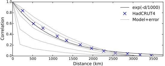
The correlation between grid cell values as a function of distance was deter-mined by the following steps: Monthly gridded temperature anomalies were used for grid cells and months of the year where at least 10 values are available over the period 1981-2010. The values were detrended to remove any climate signal, and normalized to zero mean and unit variance, giving a detrended anomaly for each grid cell and month of the year. Squared differences between cells were then accumulated as a function of the distance between the cells. The resulting function is well described by an exponential function with only a single param-eter; the length-scale (Figure 1). A preliminary value for the length-scaled0 in

Equation 6 was determined by least squares optimization to fit the predicted to the observed correlation for pairs of observations within 4000 km, giving a best estimate ford0of≈1000 km. However the range over which temperatures

0 500 1000 1500 2000 2500 3000 3500 Dιστανχε (κm)

0.0 0.2 0.4 0.6 0.8 1.0

Χ

ο

ρρ

ε

λα

τι

ο

ν

εξπ(−δ/1000) ΗαδΧΡΥΤ4 Μοδελ+ερρορ

Figure 1: Correlation as a function of distance estimated from pairwise compar-ison of cells from the HadCRUT4 blended land/ocean data. Crosses indicate binned averages. The thick line is the least squares fit of an exponential func-tion against every individual cell difference. Thin lines show the correlafunc-tion with distance for the MERRA2 reanalysis with spatially constant geographical noise of 0.25◦_{C (top line), 0.5}◦_{C, 1.0}◦_{C, 2.0}◦_{C, 5.0}◦_{C (bottom line).}

specifictemperature field can vary depending on the distribution of unobserved cells and will be determined later by simulation.

The correlation between observations is influenced both by the distance be-tween the observations and by the noise in the individual observations. To isolate the effect of noise, correlograms were also determined for surface tem-perature fields from the MERRA2 reanalysis (Gelaro et al., 2017), a recently developed atmospheric reanalysis spanning 1980 to the present. Figure 1 also shows how correlation changes with distance for the MERRA2 reanalysis data with different amounts of geographically constant noise. When the noise signal is small, the correlogram has a bell curve shape. Increasing noise scales the correlations for all distances greater than zero, and so the fit to the exponential model is somewhat contingent on the magnitude of the noise contribution. The observed correlogram falls between the reanalysis correlograms for a noise con-tribution of between 0.5 and 1.0◦_{C, consistent with estimates from Morice et al.}

(2012) for the size of this term in real world data.

The GTA1 method includes several simplifications which might impact the efficiency of the estimator. The method will therefore be tested by reconstruct-ing temperature fields from incomplete and noisy data where the correct answer is known. The MERRA2 reanalysis was used for this purpose, however the ERA-interim reanalysis (Dee et al., 2011), which shows faster Arctic warming over recent years (Simmons and Poli, 2015; Simmons et al., 2017), leads to sim-ilar conclusions.

The validation method follows a similar approach to that used in the estima-tion of coverage uncertainty in the HadCRUT family of temperature products (Jones et al., 1997; Brohan et al., 2006; Morice et al., 2012):

anomaly using a 30 year baseline period and converted to the same grid as the observational record.

• A ‘true’ global mean surface temperature anomaly is calculated from the spatially complete reanalysis field.

• Coverage is reduced to match a month from the observational record, and random noise is added to each grid cell in the reanalysis field. A global mean surface temperature estimate is then constructed from the coverage reduced noisy data using the estimator to be tested. The root-mean-squared (RMS) error between the estimate and the true value, evaluated using multiple months of data from the reanalysis, is used to evaluate the estimator.

Each month in the observational record produces a coverage mask. This mask is used in conjunction with the corresponding month from every year in the reanalysis to produce an error estimate for a given estimator. For example, for the observational coverage from January 1940, the reanalysis fields for the 37 Januaries between 1980 and 2016 are used in estimating the errors. This assumes that the spatial scale of variability is invariant under transient climate change; this assumption will be tested later using a longer reanalysis.

The validation method is contingent on the use of realistic estimates of the noise to be added to each grid cell in the reanalysis data. While the Had-CRUT4 dataset provides uncertainty estimates for each individual grid cell (Morice et al., 2012), these estimates do not include contributions from tem-porally and spatially correlated biases in the land and sea surface temperature observations, which are instead provided through an ensemble of reconstructions and covariance matrices (Kennedy et al., 2011; Morice et al., 2012).

An independent estimate for the cell noise including all of the relevant contri-butions was therefore determined from the temperature data themselves. A 3×3 block of grid cells was omitted from the map, and the value for the centre cell of the omitted region restored by kriging using the method of Cowtan and Way (2014). The error in the cell value was then estimated from the difference be-tween the observed and reconstructed values. The calculation was repeated for each cell in turn. The RMS error for a given cell was then estimated from the root mean square of the errors (over time) in that cell, for those cells with at least 60 months of differences over the period 1981-2010.

The errors in isolated Antarctic observations are overestimated because there are no nearby stations, and the noise estimate therefore contains a significant contribution from the geographical differences between stations. The maximum value for the cell noise was therefore capped at the 99th percentile of the values obtained over the whole map, with the result that the inland Antarctic cells were given a similar error to cells in the Arctic. The resulting noise map is shown in Figure 2. For cells where insufficient data were available to estimate the error, RMS error values were extrapolated by kriging.

0.0 0.2 0.4 0.6 0.8 1.0 1.2 1.4 1.6 1.8 2.0

Figure 2: Root mean squared error in ◦_{C in the HadCRUT4 data estimated}

from the difference between the value of a cell and a value inferred from nearby (but non-neighbouring) cells by kriging. Data are for the period 1981-2010.

50% larger in size: this reflects the facts that some of the error sources identi-fied by Morice et al. are not included in the comparison, and that our estimates are inflated by interpolation error. Noise will be larger for earlier periods be-cause there are often fewer observations per grid cell; however when identifying climatic contributions to coverage bias annual and decadal error estimates are more relevant than the monthly estimates used here. On this basis the noise estimates are likely to be conservative for recent decades but may be underesti-mated for the early record. Our noise estimates do not include the effects of long range spatial correlated biases which are represented in the HadCRUT4 by an ensemble of temperature realizations, because while these contribute to the total uncertainty in the global mean temperature anomaly they have comparatively little impact on the contribution of incomplete coverage to that uncertainty.

The noise map was used to add uncorrelated noise series to each cell in the reanalysis data from a normal distribution with mean of zero and standard deviation equal to the estimated RMS error for that cell. This does not account for the partial correlation of the errors in the sea surface temperature data, which may lead to the impact of noise in the data being slightly underestimated.

To determine the optimum value of the length-scale d0 the errors in the

GTA1 estimator were evaluated for length-scales in the range 500-1500 km. The RMS error in the GTA1 estimate as a function of length-scale is shown in Figure 3. The results from reconstructing the reanalysis data support a value of between 800 and 900 km ford0, similar to but slightly lower than the value

determined from the observations.

500 700 900 1100 1300 1500 Ραδιυσ (κm)

0.033 0.034 0.035 0.036 0.037

Ρ

Μ

Σ

ε

ρρ

ο

ρ

(°

Χ

)

Figure 3: Root mean squared error in global mean surface temperature estimates as a function of length-scaled0 for the GTA1 estimator. The error is evaluated

by reducing the coverage of every year of the MERRA2 reanalysis data to match the coverage of the HadCRUT4 observations for the years 1981-2010.

−90 −60 −30 0 30 60 90

Λατιτυδε (°Ν) 0.0000

0.0001 0.0002 0.0003 0.0004 0.0005 0.0006 0.0007

Χ

ε

λλ

ω

ε

ιγ

η

τ

Χελλ αρεα ΓΤΑ1(250κm) ΓΤΑ1(800κm)

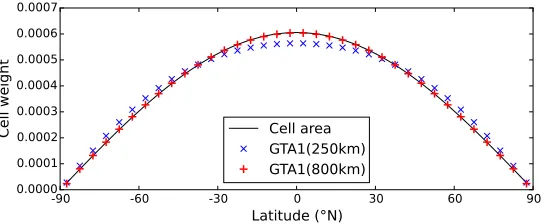
Figure 4: Weights given to grid cells as a function of latitude in the case of a spatially complete field by a simple weighted average based on cell area, and by the GTA1 estimator withe-folding radiusd0 of 250 km or 800 km.

greater than the cell spacing: values ofd0 which are significantly less than the

cell spacing lead to cell weights which diverge from the cell areas, approaching uniform (i.e. non-area) weighting asd0 tends to zero. The equivalence to area

weighting is also contingent on the use of the correlation matrix rather than the covariance matrix in Equation 5, otherwise regions with noisier observations are systematically downweighted.

4

Results

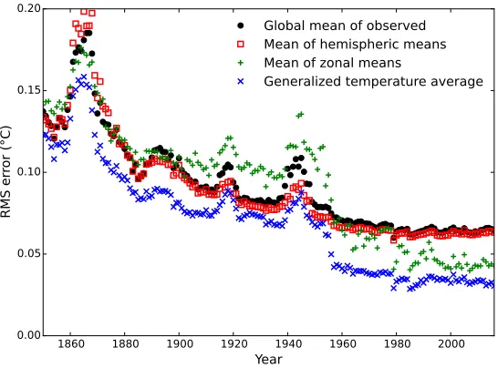
1. The global mean of the observed cells, which is the method used in combi-nation with different levels of infilling by Vose et al. (2012), Hansen et al. (2010) and Japan Meterological Agency (2017).

2. The mean of the hemispheric means of the observed cells, which is the method used by Morice et al. (2012).

3. The mean of the zonal means, which has been used for radiosonde data by Thorne et al. (2005) and for surface temperature data by Gleisner et al. (2015) under the assumption that temperature anomalies are primarily correlated with other temperature anomalies at the same latitude.

4. The generalized least squares estimator GTA1 described by Equations 5 and 6, with the length-scaled0set to 800 km.

The RMS errors for the four different global mean estimators are plotted for the coverage of each month in the HadCRUT4 record in Figure 5. The global mean of the observed cells and the mean of the hemispheric means lead to very similar RMS errors, with the mean of the hemispheric means performing slightly better during the mid-20th century but worse during the 19th century. The mean of the zonal means performs substantially better than the global or hemispheric means for the period since 1950, however it performs worse than these methods prior to that date. The GTA1 estimator performs better than all the other estimators over the whole of the record, and in particular leads to RMS errors which are about half of the error from the global or hemispheric means for recent years. Since errors combine as variances this implies that use of the GTA1 estimator mitigates three quarters of the error variance from sampling and measurement errors in the global or hemispheric means.

The difference between the generalized least squares average and the simple area weighted average may be understood by examining the weights given under the GTA1 approach to different cells, illustrated using the data from January 1920 of the CRUTEM4 land temperature dataset (Jones et al., 2012), normal-ized such that the largest weight is equal to one (Figure 6). Isolated observations are given unit weight. Isolated pairs of adjacent observations are given just over half weight. Densely sampled observations are further downweighted inversely with the density of observations, to produce an effective area weighting.

1860 1880 1900 1920 1940 1960 1980 2000 Ψεαρ

0.00 0.05 0.10 0.15 0.20

Ρ

Μ

Σ

ε

ρρ

ο

ρ

(°

Χ

)

Γλοβαλ mεαν οφ οβσερϖεδ Μεαν οφ ηεmισπηεριχ mεανσ Μεαν οφ ζοναλ mεανσ

Γενεραλιζεδ τεmπερατυρε αϖεραγε

Figure 5: Root mean squared error in global mean surface temperature estimates as a function of coverage. The four estimators are compared on the basis of the error in reconstructing coverage reduced MERRA2 data, where coverage is determined by each of 12 months of a given year in the HadCRUT4 data.

0.0 0.1 0.2 0.3 0.4 0.5 0.6 0.7 0.8 0.9 1.0

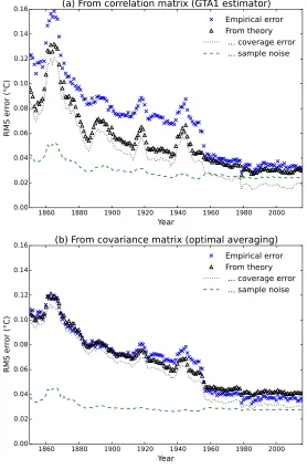
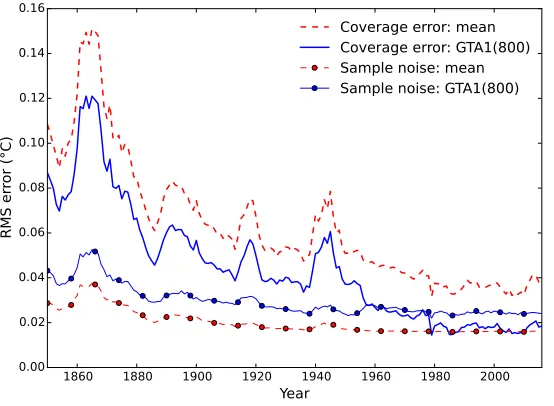
A theoretical estimate of the expected coverage error can be obtained from Equation 9. However this estimate does not include the contribution of sample noise arising from errors in the observations, which is present even when coverage is complete and so Var( ˆT) is zero. The contribution of sample noise to the error in ˆT can be estimated using Equation 10 from the cell weights wGLS and the

diagonal matrix Σ whose diagonal elements are the estimated noise variances for each grid cell, determined empirically from the observations as described in Section 3 (Kagan, 1997, Equation 3.1.5).

Varnoise( ˆT) =wGLS⊤ ΣwGLS (10)

The total error variance of the GTA1 estimator should be given by the sum of Var( ˆT) and Varnoise( ˆT). This estimate of the uncertainty in the GTA1

esti-mator, along with the contributory terms, is compared to the empirical RMS error in Figure 7(a). The theoretical estimate of the uncertainty in the esti-mator agrees well with the empirical values for the period from the late 1950s when Antarctic observations are available, but underestimates the uncertainty for the earlier periods, which suggests that the correlation model is too simple to produce optimal results for the early part of the record.

The correlation matrixCcan be converted into a covariance matrix by mul-tiplying each row and column by the standard deviations of the temperature anomalies for the corresponding grid cells. However if the covariance matrix is used in Equation 5, the resulting weights do not tend towards the cell areas as coverage improves. Correct determination of the weights from the covariance matrix requires the more complex normalization procedure of Kagan (1997, Equation 3.3.7) or Weber and Madden (1995, Equation 13) (the additional nor-malization has no effect if applied to the correlation matrix). Figure 7(b) shows the theoretical and empirical uncertainties estimates obtained when using the covariance matrix, which now show good agreement over the whole period. While performance of the correlation and covariance calculations is similar for recent decades, use of the covariance matrix noticeably reduces the errors in the early period. If coverage is poor and complexity is not an issue, the full optimal averaging method of Kagan should therefore be used in preference to the simpler GTA1 estimator.

The same approach can be used to analyse the errors for the other estimators by substituting the effective cell weights for that estimator in place of wGLS.

1860 1880 1900 1920 1940 1960 1980 2000 Ψεαρ

0.00 0.02 0.04 0.06 0.08 0.10 0.12 0.14 0.16

Ρ

Μ

Σ

ε

ρρ

ο

ρ

(°

Χ

)

(α) Φροm χορρελατιον mατριξ (ΓΤΑ1 εστιmατορ)

Εmπιριχαλ ερρορ Φροm τηεορψ ... χοϖεραγε ερρορ ... σαmπλε νοισε

1860 1880 1900 1920 1940 1960 1980 2000 Ψεαρ

0.00 0.02 0.04 0.06 0.08 0.10 0.12 0.14 0.16

Ρ

Μ

Σ

ε

ρρ

ο

ρ

(°

Χ

)

(β) Φροm χοϖαριανχε mατριξ (οπτιmαλ αϖεραγινγ)

Εmπιριχαλ ερρορ Φροm τηεορψ ... χοϖεραγε ερρορ ... σαmπλε νοισε

1860 1880 1900 1920 1940 1960 1980 2000 Ψεαρ

0.00 0.02 0.04 0.06 0.08 0.10 0.12 0.14 0.16

Ρ

Μ

Σ

ε

ρρ

ο

ρ

(°

Χ

)

Χοϖεραγε ερρορ: mεαν Χοϖεραγε ερρορ: ΓΤΑ1(800) Σαmπλε νοισε: mεαν Σαmπλε νοισε: ΓΤΑ1(800)

Figure 8: Comparison of the coverage error and sample noise contributions for both the global mean of the observed cells and the GTA1 estimators.

of the GTA1 estimator over the global mean of the observed cells arises from a better compromise between these two sources of error.

In contrast to Kagan (1979), the noise contribution of individual cell values to the global mean is not handled explicitly in the GTA1 estimator, rather the global scale of the noise contribution is handled through the length-scale of the correlogramd0, although the fit of the exponential model becomes poorer with

lower or higher noise levels than those in the HadCRUT4 observations (Figure 1). In the absence of noise, inclusion of an isolated cell observation reduces the uncertainty in the resulting global mean in proportion to the area of the planet for which that observation is informative, which is controlled by the length-scale. Since uncertainties sum in quadrature they are dominated by the larger source of error, thus when the noise is less than the bias which is mitigated by including that cell, the cell noise has little effect on the correlogram. If the cell noise exceeds the bias mitigated by including that cell, the optimal range for the correlogram drops rapidly, with the effect that multiple observed cells are required to provide an informative temperature estimate for the same area.

4.1

Contributions to coverage uncertainty

Coverage uncertainty in a global mean temperature estimate from spatially incomplete data arises from two sources: changes in the temperature of the unobserved region relative to the observed region, and changes in coverage. Let

of the observed region,Tunobsbe the mean temperature of the unobserved region, andfunobs be the fraction of the surface which is unobserved. Then:

Tgl=Tobs(1−funobs) +Tunobsfunobs. (11)

If the mean temperature is estimated from the average of the observed region alone, the error in the resulting estimate will beǫ=Tobs−Tgl. Let the difference between the means of the unobserved and observed regions beDunobs =Tobs− Tunobs, then:

ǫ=Dunobsfunobs. (12)

When using temperature anomalies, the absolute value of the bias is irrelevant, however changes in bias over time will lead to an error in temperature trends spanning the change in bias. The change in bias obeys a product rule:

δǫ≈Dunobsδfunobs+funobsδDunobs. (13)

Therefore a change in coverage bias may arise from a change in the difference between the temperatures of observed and unobserved regions, or from a change in coverage subject toDunobs being non-zero.

Changes in Dunobs may be noise-like, for example due to weather systems moving into or out of the unobserved region, or bias-like, for example due to relative changes in climate between the observed and unobserved regions relative to the baseline period. The rapid warming of the incompletely observed Arctic is an example of the latter (Cowtan and Way, 2014), although decadal scale regional climate change due to internal variability has been shown to occur elsewhere as well (Xie et al., 2015).

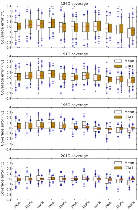
To separate the effects of changes in climate and changes in coverage, addi-tional validation tests were performed in which the coverage for a given month was used to calculate the error due to limited coverage in a historical reanalysis temperature field for the corresponding month only. The ERA 20th Century Reanalysis (ERA20C) was used for this experiment (Poli et al., 2013), and pro-vides a spatially complete temperature field covering the period 1900-2010. The reanalysis is based on temperature, pressure and wind observations from the oceans, and pressure and wind observations from land weather stations. How-ever for unsampled regions (such as Antarctica in the early 20th century) the reanalysis temperatures are determined solely by the atmospheric model and boundary conditions, and may also be impacted by observational biases. No noise was added to ERA20C reanalysis data.

the spread of the errors reduced. With 2010 coverage bias is almost eliminated and the spread of the errors substantially reduced.

Bias is expected to be lower during the 1961-1990 baseline period because

Dunobs should be close to zero, but in practice only the 1970s temperature estimates show little bias when using the global mean estimator. The spread in the errors due to the weather contribution to coverage error is large compared to the persistent climatic contribution, however there is a centennial trend from a warm to a cool bias in the global mean estimator for all coverages, and in the GTA1 estimator for 1860 and 1910 coverage due to the faster warming of the unobserved regions (Simmons et al., 2010). The global mean consistently underestimates the warming in the reanalysis data for any historical coverage. The GTA1 estimator provides a good estimate of the rate of warming for 1960 or 2010 coverage, but underestimates the rate of warming when limited to 1860 or 1910 coverage.

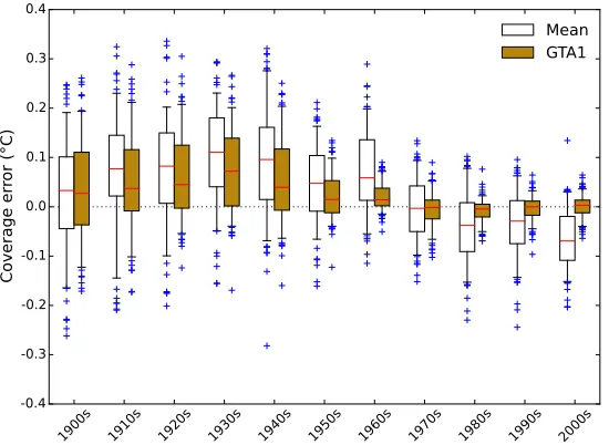
Figure 10 shows the the same experiment but using the historical coverage for the corresponding month as the basis for temperature reconstruction. For the period since the 1950s bias is near zero and noise is dramatically reduced by the GTA1 estimator. For earlier decades the GTA1 estimator provides a modest reduction in bias but little reduction in noise. The bias tends to be undercorrected suggesting that the GTA1 estimator is conservative with respect to the magnitude of the bias correction.

Changes in bias when using fixed coverage (Figure 9) arise from changes in temperature anomaly in the unobserved region relative to the observed region, while the changes in bias when using historical coverage include the additional contribution from changes in coverage. The most notable change in the 1950s is the establishment of the Antarctic weather stations. The GTA1 estimator leads to consistently low noise and bias with 2010 coverage, however it does not significantly reduce noise and only mitigates some bias with pre-1950 coverage. The actual bias estimates are however contingent on the reanalysis produc-ing realistic temperatures in regions where no weather station observations are present.

4.2

Impact of temperature estimators on the global

warm-ing “hiatus”

Numerous research papers have discussed a possible “hiatus” in global warm-ing at the start of the 21st century (Lewandowsky et al., 2015; Medhaug et al., 2017). The IPCC Fifth Assessment Report noted a trend in the HadCRUT4 temperature record of 0.04◦_{C/decade for the period 1998-2012 (Hartmann et al.,}

2013). This trend is substantially below the 32 year trend of about 0.17◦_C/decade

−0.4 −0.3 −0.2 −0.1 0.0 0.1 0.2 0.3 0.4 Χ ο ϖ ε ρα γ ε ε ρρ ο ρ (° Χ ) 1860 χοϖεραγε −0.4 −0.3 −0.2 −0.1 0.0 0.1 0.2 0.3 0.4 Χ ο ϖ ε ρα γ ε ε ρρ ο ρ (° Χ ) 1910 χοϖεραγε Μεαν ΓΤΑ1 −0.4 −0.3 −0.2 −0.1 0.0 0.1 0.2 0.3 0.4 Χ ο ϖ ε ρα γ ε ε ρρ ο ρ (° Χ ) 1960 χοϖεραγε Μεαν ΓΤΑ1 1900 σ 1910 σ 1920 σ 1930 σ 1940 σ 1950 σ 1960 σ 1970 σ 1980 σ 1990 σ 2000 σ −0.4 −0.3 −0.2 −0.1 0.0 0.1 0.2 0.3 0.4 Χ ο ϖ ε ρα γ ε ε ρρ ο ρ (° Χ ) 2010 χοϖεραγε Μεαν ΓΤΑ1

1900 σ

1910 σ

1920 σ

1930 σ

1940 σ

1950 σ

1960 σ

1970 σ

1980 σ

1990 σ

2000 σ

−0.4 −0.3 −0.2 −0.1 0.0 0.1 0.2 0.3 0.4

Χ

ο

ϖ

ε

ρα

γ

ε

ε

ρρ

ο

ρ

(°

Χ

)

Μεαν ΓΤΑ1

Figure 10: Error in the global mean of the observed cells and the GTA1 estima-tors of global mean surface temperature, grouped by decade when reconstruct-ing months of the ERA-20C reanalysis data reconstructed usreconstruct-ing the HadCRUT4 observational coverage from the corresponding year of the observational record.

(Huang et al., 2015; Hausfather et al., 2017), and a trend from El Ni˜no to La Ni˜na conditions over the period.

Temperature trends for HadCRUT4 version 4.1.1, which was the current version at the time of preparation of Hartmann et al., and for the now current version 4.6.0 were determined using the four estimators outlined earlier to de-termine the sensitivity of the trend to the temperature averaging method. The results are shown in table 1.

Method HadCRUT4.1.1 HadCRUT4.6.0 Global mean of observed cells 0.040 0.054 Mean of hemispheric means 0.040 0.052

Mean of zonal means 0.074 0.086

GTA1(800) 0.088 0.098

Table 1: Temperature trends in ◦_{C/decade for the period 1998-2012}

(Hartmann et al., 2013) using the four different estimators of global mean sur-face temperature. Trends are given for the HadCRUT4.1.1 data, which were current at the time of Hartmann et al., and for the most recent version.

5

Discussion

Historical temperature record products are utilized for multiple purposes, some-times with conflicting requirements. Gridded temperature data are used to evaluate the performance of climate models and to identify spatial signatures associated with different climatic influences. The gridded data are also sum-marized by a global mean surface temperature estimate which may be used to quantify change in global climate for public and policy purposes, and to esti-mate cliesti-mate sensitivity in simple energy balance calculations, e.g. Otto et al. (2013).

The HadCRUT4 record provides a monthly record of gridded temperature observations, with each observation contributing to only a single map grid cell. The Japan Meteorological Agency record (Japan Meterological Agency, 2017) adopts a similar approach for land based weather stations. In contrast records from Hansen et al. (2010), Rohde et al. (2013) and Cowtan and Way (2014) use infilling to produce a temperature field with near global coverage, which may be averaged by conventional methods. The errors in the resulting averages are contingent on the effectiveness of the infilling method.

The non-infilled temperature products have an important benefit for the evaluation of climate models. The gridded temperature record can be compared to the climate model outputs after reducing coverage to match the observational record. The benefit of using a non-infilled product in this case is that differences between the models and observations must arise from either the models or the observations. By contrast when using an infilled record, differences may arise from the models, the observationsor from artifacts of the infilling method.

The simplicity of the gridded observational record leads to a product which is easier for temperature record users to understand, and if necessary to reproduce. Simple methods are easier to debug and maintain, which is important for prod-ucts which must be maintained over many years by changing personnel. There are therefore multiple reasons to maintain non-infilled gridded observational records. A simple average of the resulting gridded data however can produce misleading results, with the temperature trends during the hiatus period being a notable example.

surface temperature from spatially incomplete observations. For recent years this estimator mitigates the larger part of the error associated with the use of the naive area weighted mean. The estimator is almost identical to the use of kriging to infill to global coverage and then averaging the resulting field, however it is simpler to implement and analyse. Implementation requires around 20 lines of computer code, and the results are determined solely by the temperature field (including the coverage mask) and a single parameter which describes the range of spatial autocorrelation in the temperature field. The estimator is also less biased than the mean of the zonal means which has been used with radiosonde data.

A number of more sophisticated approaches to averaging temperature data have been proposed, from Kagan (1979) to the recent works of Ilyas et al. (2017) and Huang et al. (2017). We do not intend the simple estimator proposed here to be a replacement for such methods, however it does provide an easily un-derstood and easily analyzed demonstration of why more naive averages are inadequate. Ideally, global temperature estimation would be performed using the optimal averaging method of Kagan or more modern methods, however where simplicity of implementation and reproducibility are concerns the GTA1 estimator can still substantially reduce the coverage error contribution to tem-peratures estimates for recent decades. The impact on temperature trends dur-ing the apparent ‘hiatus’ period provides an illustration of why good statistical estimators of global mean temperature are required for use in the evaluation of both historical temperature change and current temperature trends.

Data and methods for this paper are available at

https://doi.org/10.15124/c47f6da3-2430-4f0e-973e-6f6597c6da42with updates at_{http://www-users.york.ac.uk/~kdc3/papers/coverage2018}.

Acknowledgements

Peter Thorne was partially supported by the Copernicus Climate Change Ser-vice under C3S 311a Lot 2 (Global Land and Marine Observations Database) activities. Richard Wilkinson was partially supported by the EPSRC-funded Past Earth Network (Grant number EP/M008363/1). Two reviewers provided insightful suggestions which improved the manuscript.

References

E. Anderson, Z. Bai, C. Bischof, S. Blackford, J. Demmel, J. Dongarra, J. Du Croz, A. Greenbaum, S. Hammarling, A. McKenney, and D. Sorensen. LAPACK Users’ Guide. Society for Industrial and Applied Mathematics, Philadelphia, PA, third edition, 1999. ISBN 0-89871-447-8 (paperback).

K. Cowtan and R. Way. Coverage bias in the HadCRUT4 temperature series and its impact on recent temperature trends.Quarterly Journal of the Royal Meteorological Society, 140(683):1935–1944, 2014. doi: 10.1002/qj.2297.

D. Dee, S. Uppala, A. Simmons, P. Berrisford, P. Poli, S. Kobayashi, U. Andrae, M. Balmaseda, G. Balsamo, P. Bauer, P. Bechtold, A. Beljaars, L. van de Berg, J. Bidlot, N. Bormann, C. Delsol, R. Dragani, M. Fuentes, A. Geer, L. Haimberger, S. Healy, H. Hersbach, E. Hlm, L. Isaksen, P. Kllberg, M. Khler, M. Matricardi, A. Mcnally, B. Monge-Sanz, J.-J. Morcrette, B.-K. Park, C. Peubey, P. de Rosnay, C. Tavolato, J.-N. Thpaut, and F. Vitart. The era-interim reanalysis: Configuration and performance of the data as-similation system.Quarterly Journal of the Royal Meteorological Society, 137 (656):553–597, 2011. doi: 10.1002/qj.828.

P. F. Dubois, K. Hinsen, and J. Hugunin. Numerical python. Computers in Physics, 10(3), 1996. doi: 10.1063/1.4822400.

G. Flato, J. Marotzke, B. Abiodun, P. Braconnot, S. C. Chou, W. J. Collins, P. Cox, F. Driouech, S. Emori, V. Eyring, et al. Evaluation of climate models. Climate Change 2013: The Physical Science Basis. Contribution of Working Group I to the Fifth Assessment Report of the Intergovernmental Panel on Climate Change, pages 741–866, 2013.

C. Folland, N. Rayner, S. Brown, T. Smith, S. Shen, D. Parker, I. Macadam, P. Jones, R. Jones, N. Nicholls, and D. Sexton. Global temperature change and its uncertainties since 1861. Geophysical Research Letters, 28(13):2621– 2624, 2001. doi: 10.1029/2001GL012877.

G. Foster and S. Rahmstorf. Global temperature evolution 19792010. Environmental Research Letters, 6(4):044022, 2011. URL

http://stacks.iop.org/1748-9326/6/i=4/a=044022.

L. S. Gandin. Optimal averaging of meteorological fields. Technical report, US Department of Commerce, National Oceanic and Atmospheric Administra-tion, National Weather Service, National Meteorological Center, 1993. URL

http://www.lib.ncep.noaa.gov/ncepofficenotes/files/014089EE.pdf. NOAA/NWS/NMC Office Note 397.

R. Gelaro, W. McCarty, M. J. Surez, R. Todling, A. Molod, L. Takacs, C. Ran-dles, A. Darmenov, M. G. Bosilovich, R. Reichle, K. Wargan, L. Coy, R. Cul-lather, C. Draper, S. Akella, V. Buchard, A. Conaty, A. da Silva, W. Gu, G.-K. Kim, R. Koster, R. Lucchesi, D. Merkova, J. E. Nielsen, G. Partyka, S. Pawson, W. Putman, M. Rienecker, S. D. Schubert, M. Sienkiewicz, and B. Zhao. The modern-era retrospective analysis for research and applications, version 2 (merra-2).Journal of Climate, 2017. doi: 10.1175/JCLI-D-16-0758. 1.

troposphere data. Geophysical Research Letters, 42(2):510–517, 2015. doi: 10.1002/2014GL062596.

J. Graham. Missing data analysis: Making it work in the real world.Annual Re-view of Psychology, 60:549–576, 2009. doi: 10.1146/annurev.psych.58.110405. 085530.

J. Hansen, M. Sato, R. Ruedy, K. Lo, D. Lea, and M. Medina-Elizade. Global temperature change. Proceedings of the National Academy of Sciences of the United States of America, 103(39):14288–14293, 2006. doi: 10.1073/pnas. 0606291103.

J. Hansen, R. Ruedy, M. Sato, and K. Lo. Global surface temperature change. Reviews of Geophysics, 48(4), 2010. doi: 10.1029/2010RG000345.

D. Hartmann, A. Klein Tank, M. Rusticucci, L. Alexander, S. Brnnimann, Y.-R. Charabi, F. Dentener, E. Dlugokencky, D. Easterling, A. Kaplan, B. Soden, P. Thorne, M. Wild, and P. Zhai. Observations: Atmosphere and surface. Climate Change 2013 the Physical Science Basis: Work-ing Group I Contribution to the Fifth Assessment Report of the Intergov-ernmental Panel on Climate Change, 9781107057999:159–254, 2013. doi: 10.1017/CBO9781107415324.008.

Z. Hausfather, K. Cowtan, D. C. Clarke, P. Jacobs, M. Richardson, and R. Ro-hde. Assessing recent warming using instrumentally homogeneous sea sur-face temperature records.Science Advances, 3(1), 2017. doi: 10.1126/sciadv. 1601207. URLhttp://advances.sciencemag.org/content/3/1/e1601207.

B. Huang, V. Banzon, E. Freeman, J. Lawrimore, W. Liu, T. Peterson, T. Smith, P. Thorne, S. Woodruff, and H.-M. Zhang. Extended reconstructed sea surface temperature version 4 (ERSST.v4). part i: Upgrades and intercomparisons. Journal of Climate, 28(3):911–930, 2015. doi: 10.1175/JCLI-D-14-00006.1.

J. Huang, X. Zhang, Q. Zhang, Y. Lin, M. Hao, Y. Luo, Z. Zhao, Y. Yao, X. Chen, L. Wang, and S. Nie. Recently amplified arctic warming has con-tributed to a continual global warming trend. Nature Climate Change, 7 (12):875–879, 2017. ISSN 1758-6798. doi: 10.1038/s41558-017-0009-5. URL

https://doi.org/10.1038/s41558-017-0009-5.

M. Ilyas, C. M. Brierley, and S. Guillas. Uncertainty in regional temper-atures inferred from sparse global observations: Application to a prob-abilistic classification of el nio. Geophysical Research Letters, 44(17): 9068–9074, 2017. ISSN 1944-8007. doi: 10.1002/2017GL074596. URL

http://dx.doi.org/10.1002/2017GL074596.

Japan Meterological Agency. Global average

sur-face temperature anomalies, 2017. URL

P. Jones, T. Osborn, and K. Briffa. Estimating sampling errors in large-scale temperature averages. Journal of Climate, 10(10):2548–2568, 1997. doi: 10. 1175/1520-0442(1997)010h2548:ESEILSi2.0.CO;2.

P. Jones, M. New, D. Parker, S. Martin, and I. Rigor. Surface air temperature and its changes over the past 150 years.Reviews of Geophysics, 37(2):173–199, 1999. doi: 10.1029/1999RG900002.

P. Jones, D. Lister, T. Osborn, C. Harpham, M. Salmon, and C. Morice. Hemi-spheric and large-scale land-surface air temperature variations: An extensive revision and an update to 2010.Journal of Geophysical Research Atmospheres, 117(5), 2012. doi: 10.1029/2011JD017139.

R. L. Kagan. Averaging of meteorological fields. Gidrometeoizdat,Leningrad, 1979.

R. L. Kagan. Averaging of meteorological fields. Springer, 1997.

A. Kaplan, Y. Kushnir, M. Cane, and M. Blumenthal. Reduced space optimal analysis for historical data sets: 136 years of atlantic sea surface temperatures. Journal of Geophysical Research C: Oceans, 102(C13):27835–27860, 1997.

T. Karl, A. Arguez, B. Huang, J. Lawrimore, J. McMahon, M. Menne, T. Pe-terson, R. Vose, and H.-M. Zhang. Possible artifacts of data biases in the recent global surface warming hiatus. Science, 348(6242):1469–1472, 2015. doi: 10.1126/science.aaa5632.

J. Kennedy, N. Rayner, R. Smith, D. Parker, and M. Saunby. Reassessing biases and other uncertainties in sea surface temperature observations measured in situ since 1850: 1. measurement and sampling uncertainties. Journal of Geo-physical Research Atmospheres, 116(14), 2011. doi: 10.1029/2010JD015218.

S. Lewandowsky, J. Risbey, and N. Oreskes. On the definition and identifiability of the alleged ”hiatus” in global warming. Scientific Reports, 5, 2015. doi: 10.1038/srep16784.

R. J. Little and D. B. Rubin.Statistical analysis with missing data. John Wiley & Sons, 2002.

I. Medhaug, M. Stolpe, E. Fischer, and R. Knutti. Reconciling controversies about the ’global warming hiatus’. Nature, 545(7652):41–47, 2017. doi: 10. 1038/nature22315.

A. Otto, F. Otto, O. Boucher, J. Church, G. Hegerl, P. Forster, N. Gillett, J. Gregory, G. Johnson, R. Knutti, N. Lewis, U. Lohmann, J. Marotzke, G. Myhre, D. Shindell, B. Stevens, and M. Allen. Energy budget constraints on climate response. Nature Geoscience, 6(6):415–416, 2013. doi: 10.1038/ ngeo1836.

P. Poli, H. Hersbach, D. G. H. Tan, D. Dee, J.-J. Thepaut, A. Simmons, C. Peubey, P. Laloyaux, T. Komori, P. Berrisford, R. Dragani, Y. Tr´emolet, E. V. H´olm, M. Bonavita, L. Isaksen, and M. Fisher. The data assimilation system and initial performance evaluation of the ecmwf pilot reanalysis of the 20th-century assimilating surface observations only (era-20c). Shinfield Park, Reading, September 2013.

J. Rennie, J. Lawrimore, B. Gleason, P. Thorne, C. Morice, M. Menne, C. Williams, W. G. Almeida, J. Christy, M. Flannery, , and M. Ishihara. The international surface temperature initiative global land surface databank: Monthly temperature data release description and methods.Geoscience Data Journal, 1(2):75–102, 2014.

R. Rohde, R. Muller, R. Jacobsen, S. Perlmutter, A. Rosenfeld, J. Wurtele, J. Curry, C. Wickhams, and S. Mosher. Berkeley earth temperature averaging process. Geoinfor. Geostat.: An Overview, 13:20–100, 2013.

S. S. Shen, G. R. North, and K.-Y. Kim. Spectral approach to optimal estima-tion of the global average temperature. Journal of Climate, 7(12):1999–2007, 1994.

A. Simmons and P. Poli. Arctic warming in era-interim and other analyses. Quarterly Journal of the Royal Meteorological Society, 141(689):1147–1162, 2015. doi: 10.1002/qj.2422.

A. Simmons, K. Willett, P. Jones, P. Thorne, and D. Dee. Low-frequency variations in surface atmospheric humidity, temperature, and precipita-tion: Inferences from reanalyses and monthly gridded observational data sets. Journal of Geophysical Research Atmospheres, 115(1), 2010. doi: 10.1029/2009JD012442.

A. Simmons, P. Berrisford, D. Dee, H. Hersbach, S. Hirahara, and J.-N. Thpaut. A reassessment of temperature variations and trends from global reanalyses and monthly surface climatological datasets. Quarterly Journal of the Royal Meteorological Society, 143(702):101–119, 2017. doi: 10.1002/qj.2949.

T. Smith, R. Reynolds, T. Peterson, and J. Lawrimore. Improvements to noaa’s historical merged land-ocean surface temperature analysis (1880-2006). Jour-nal of Climate, 21(10):2283–2296, 2008. doi: 10.1175/2007JCLI2100.1.

T. F. Stocker, D. Qin, G.-K. Plattner, M. Tignor, S. K. Allen, J. Boschung, A. Nauels, Y. Xia, B. Bex, and B. Midgley. Ipcc, 2013: climate change 2013: the physical science basis. contribution of working group i to the fifth assessment report of the intergovernmental panel on climate change, 2013.

P. Thorne, D. Parker, S. Tett, P. Jones, M. McCarthy, H. Coleman, and P. Brohan. Revisiting radiosonde upper air temperatures from 1958 to 2002. Journal of Geophysical Research D: Atmospheres, 110(18):1–17, 2005. doi: 10.1029/2004JD005753.

K. Y. Vinnikov, P. Y. Groisman, and K. Lugina. Empirical data on contem-porary global climate changes (temperature and precipitation). Journal of Climate, 3(6):662–677, 1990.

R. Vose, D. Wuertz, T. Peterson, and P. Jones. An intercomparison of trends in surface air temperature analyses at the global, hemispheric, and grid-box scale. Geophysical Research Letters, 32(18):1–4, 2005. doi: 10.1029/ 2005GL023502.

R. Vose, D. Arndt, V. Banzon, D. Easterling, B. Gleason, B. Huang, E. Kearns, J. Lawrimore, M. Menne, T. Peterson, R. Reynolds, T. Smith, C. Williams Jr., and D. Wuertz. Noaa’s merged land-ocean surface temperature analysis. Bul-letin of the American Meteorological Society, 93(11):1677–1685, 2012. doi: 10.1175/BAMS-D-11-00241.1.

R. O. Weber and R. A. Madden. Optimal averaging for the determination of global mean temperature: experiments with model data. Journal of climate, 8(3):418–430, 1995.