temperature estimators
.
White Rose Research Online URL for this paper:
http://eprints.whiterose.ac.uk/133034/
Version: Published Version
Article:
Cowtan, K., Jacobs, P., Thorne, P. et al. (1 more author) (2018) Statistical analysis of
coverage error in simple global temperature estimators. Dynamics and Statistics of the
Climate System, 3 (1). dzy003. ISSN 2059-6987
https://doi.org/10.1093/climsys/dzy003
© The Author(s) 2018. Published by Oxford University Press. This is an Open Access
article distributed under the terms of the Creative Commons Attribution License
(http://creativecommons.org/licenses/by/4.0/), which permits unrestricted reuse,
distribution, and reproduction in any medium, provided the original work is properly cited.
[email protected]
https://eprints.whiterose.ac.uk/
Reuse
This article is distributed under the terms of the Creative Commons Attribution (CC BY) licence. This licence
allows you to distribute, remix, tweak, and build upon the work, even commercially, as long as you credit the
authors for the original work. More information and the full terms of the licence here:
https://creativecommons.org/licenses/
Takedown
If you consider content in White Rose Research Online to be in breach of UK law, please notify us by
© The Author(s) 2018. Published by Oxford University Press.
doi:10.1093/climsys/dzy003 Advance Access Publication Date: 20 July 2018 Research Article
Research Article
Statistical analysis of coverage error in simple
global temperature estimators
Kevin Cowtan
a,*
, Peter Jacobs
b, Peter Thorne
cand Richard Wilkinson
da
Department of Chemistry, University of York, York, UK,
bDepartment of Environmental Science and Policy,
George Mason University, Fairfax, VA, USA,
cICARUS, Maynooth University, Maynooth, Ireland and
dSchool
of Maths and Statistics, University of Sheffield, Sheffield, UK.
*Correspondence Kevin Cowtan, Department of Chemistry, University of York, Heslington, York, YO10 5DD, UK; E-mail: kevin.cowtan@ york.ac.uk
Received 20 December 2017; Accepted 14 July 2018
Abstract
Background. Global mean surface temperature is widely used in the climate literature as a measure of the impact of human activity on the climate system. While the concept of a spatial average is simple, the estimation of that average from spatially incomplete data is not. Correlation between nearby map grid cells means that missing data cannot simply be ignored. Estimators that (often implicitly) assume uncorrelated observations can be biased when naively applied to the observed data, and in particular, the commonly used area weighted average is a biased estimator under these circumstances. Some surface temperature products use different forms of inilling or imputation to estimate temperatures for regions distant from the nearest observation, however the impacts of such methods on estimation of the global mean are not necessarily obvious or themselves unbiased. This issue was addressed in the 1970s by Ruvim Kagan, however his work has not been widely adopted, possibly due to its complexity and dependence on subjective choices in estimating the dependence between geographically proximate observations.
Objectives. The aim of this work is to present a simple estimator for global mean surface temperature from spatially incomplete data which retains many of the beneits of the work of Kagan, while being fully speciied by two equations and a single parameter. The main purpose of the simpliied estimator is to better explain to users of temperature data the problems associated with estimating an unbiased global mean from spatially incomplete data, however the estimator may also be useful for problems with speciic requirements for reproducibility and performance.
Methods. The new estimator is based on generalized least squares, and uses the correlation matrix of the observations to weight each observation in accordance with the independent information it contributes. It can be implemented in fewer than 20 lines of computer code. The performance of the estimator is evaluated for different levels of observational coverage using reanalysis data with artiicial noise.
Results. For recent decades the generalized least squares estimator mitigates most of the error associated with the use of a naive area weighted average. The improvement arises from the fact
This is an Open Access article distributed under the terms of the Creative Commons Attribution License (http://creativecommons.org/licenses/by/4.0/), which permits unrestricted reuse, distribution, and reproduction in any medium, provided the original work is properly cited.
D
o
w
n
lo
a
d
e
d
fro
m
h
ttp
s:
//a
ca
d
e
mi
c.
o
u
p
.co
m/
cl
ima
te
syst
e
m/
a
rt
icl
e
-a
b
st
ra
ct
/3
/1
/d
zy0
0
3
/5
0
5
6
4
3
4
b
y
U
n
ive
rsi
ty
o
f S
h
e
ffi
e
ld
u
se
r
o
n
1
0
O
ct
o
b
e
r
2
0
1
that coverage bias in the historical temperature record does not arise from an absolute shortage of observations (at least for recent decades), but rather from spatial heterogeneity in the distribution of observations, with some regions being relatively undersampled and others oversampled. The estimator addresses this problem by reducing the weight of the oversampled regions, in contrast to some existing global temperature datasets which extrapolate temperatures into the unobserved regions. The results are almost identical to the use of kriging (Gaussian process interpolation) to impute missing data to global coverage, followed by an area weighted average of the resulting ield. However, the new formulation allows direct diagnosis of the contribution of individual observations and sources of error. Conclusions. More sophisticated solutions to the problem of missing data in global temperature estimation already exist. However the simple estimator presented here, and the error analysis that it enables, demonstrate why such solutions are necessary. The 2013 Fifth Assessment Report of the Intergovernmental Panel on Climate Change discussed a slowdown in warming for the period 1998-2012, quoting the trend in the HadCRUT4 historical temperature dataset from the United Kingdom Meteorological Ofice in collaboration with the Climatic Research Unit of the University of East Anglia, along with other records. Use of the new estimator for global mean surface temperature would have reduced the apparent slowdown in warming of the early 21st century by one third in the spatially incomplete HadCRUT4 product.
Key words: Climate change, historical temperature record, observational coverage.
1. Introduction
Global mean surface temperature change is a key metric in the quantiication of global warming (Stocker et al., 2013). Surface air temperature is signiicantly inluenced by local and seasonal factors, such as altitude, exposure and surface type, so the metric is usually expressed in the form of a global mean surface temperature anomaly, which is the areal average of the temperature deviation from an average over some reference period of the temperatures for that loca-tion and month of the year (Jones et al., 1999). The global mean surface temperature anomaly is then deined as the areal average of these local temperature anomalies over the whole of the surface of the planet (Equation 1), where Tgl is the global mean surface temperature anomaly for a given month, T(λ, ϕ) is the anomaly at a given latitude λ and longitude ϕ and A is the area element.
T T dA
dA ( , ) gl
∫ ∫
∫ ∫
λ φ
= (1)
For numerical purposes, temperature ields are commonly represented on a grid, most frequently a rectangular array on the latitude and longitude coordinates, although sometimes equal area grids, which feature fewer cells per latitude band at higher latitudes, are used. When we have complete data (i.e. no missing grid cells), the global mean surface temperature anomaly can be calculated from the gridded temperature anomalies under the assumption that the grid cells are small enough to accurately represent the spatial variation in the surface temperature anomaly (or that the grid cell values are themselves representative of the average temperature in the region spanned by the grid cell). The
global mean is given by Equation 2, where Ti is the temperature in a given grid cell and ai is the area of the grid cell
denoted by the index i:
=
T a T
a w T
i i i
i i
gl≈ gl
∑
∑ (2)
where wgl is the vector of normalized weights ai ⁄ ∑iai, and T is the vector of temperatures Ti.
However, observational data typically do not have global coverage, i.e. there are grid cells for which the measure-ments are missing. In the simple case where all the grid cells are uncorrelated, we could view the partial coverage as a random sample from a population. Then the best estimator of the global mean would be the sample mean (i.e. the
D
o
w
n
lo
a
d
e
d
fro
m
h
ttp
s:
//a
ca
d
e
mi
c.
o
u
p
.co
m/
cl
ima
te
syst
e
m/
a
rt
icl
e
-a
b
st
ra
ct
/3
/1
/d
zy0
0
3
/5
0
5
6
4
3
4
b
y
U
n
ive
rsi
ty
o
f S
h
e
ffi
e
ld
u
se
r
o
n
1
0
O
ct
o
b
e
r
2
0
1
mean of the available grid cells weighted by the cell areas), and this will be an unbiased estimator of the global mean surface temperature anomaly.
In practice, the observations (or more strictly the deviations from the global mean) are spatially correlated (Vinnikov et al., 1990), which complicates matters. It is useful here to introduce terminology from the statistics litera-ture (Little and Rubin, 2002; Graham, 2009), where a distinction is made between data that are missing completely at random (MCAR), missing at random (MAR) and missing not at random (MNAR). Missing data are MCAR if the missingness mechanism is independent of other information, in our case, if the probability a grid cell record is missing does not depend upon a cell’s location or the temperature anomaly. The data are MAR if the missingness depends upon the covariates, but not the quantity of interest, i.e. the probability a cell record is missing can depend upon its latitude and longitude but not the temperature anomaly. MNAR data occur when the missing mechanism depends on the quantity of interest, for example, if a temperature observation was censored for being too high or low. Only MCAR data can be analysed using complete data techniques by simply ignoring the missing values. In particular, the use of the sample mean as an estimator for the global mean is contingent on the assumptions of ordinary least squares, namely that observations are a random sample from the population and that the errors are uncorrelated, or in other words that the missing data are MCAR. When applied to MAR and MNAR data, the sample mean can lead to biased estimates. For the temperature data, missingness is strongly correlated with longitude and latitude, with, for example, data at high latitudes more likely to be missing. The observations are, therefore, at best missing conditionally at random (MAR), so that unless we control for the inluence of longitude and latitude, statistical estimators based on the data will be biased. The observations could also be MNAR due to manual station selection or outlier rejection; however, the resulting biases would not be detectable or correctable without reference to a larger set of weather sta-tion data such as that of Rohde et al. (2013) or Rennie et al. (2014).
Historical temperature records based on gridded observations include the HadCRUT4 record from the UK
Meteorological Ofice and University of East Anglia (Morice et al., 2012) and the weather station contribution to
the Japan Meteorological Agency record (Japan Meteorological Agency, 2017); however, in both cases, the global mean is determined from the mean of the grid cells for which values are available (with an additional step to equal-ize the weight of the hemispheres in the case of Morice et al.). More sophisticated methods developed for dealing with missing temperature data assume a MAR mechanism, and then try to compensate for the missing data either by using a more sophisticated estimator for the global mean or by imputing the missing data before using complete data techniques. For example, the variance-covariance matrix of observations is used directly in the optimal
estima-tion of global mean surface temperature by Kagan (1979, 1997) and has also been employed by Vinnikov et al.
(1990), Gandin (1993), Smith et al. (1994) and Weber and Madden (1995). In contrast, Hansen et al. (2010), Vose et al. (2012), Rohde et al. (2013) and Cowtan and Way (2014) use interpolation methods to reconstruct temperature estimates for the unobserved regions, although in the case of Vose et al., polar regions are not interpolated. Even in interpolated records, coverage is typically incomplete prior to the mid-20th century because many interpolation techniques only inill within a speciied distance of the available observational constraint, and that constraint is very sparse prior to the beginning of the 20th century.
Reconstruction of the global temperature ield based on empirical orthogonal functions (EOFs) is an alternative approach which introduces empirical information about the underlying physical processes through the identiication of common spatial patterns of temperature variation in the historical data (Shen et al., 1994; Kaplan et al., 1997; Folland et al., 2001). However, EOF-based methods are either limited to reconstructing temperatures in regions for which observations are available for at least part of the record or must use and become contingent on reanalyses or climate models to infer global patterns. While this may lead to superior temperature reconstructions when teleconnections are correctly diagnosed, it carries additional costs in terms of complexity and reproducibility when compared to optimal averaging and may lead to worse results if the reanalysis or model behaviour differs substantively from reality.
Why is optimal averaging not used in the historical temperature record products? Optimal averaging brings a cost in terms of complexity. Complex methods are harder to debug, harder to maintain, harder for other researchers to reproduce and less transparent to users of the data. In the absence of evidence that a simple statistic is inadequate for a particular purpose, there are, therefore, good reasons to favour a simple statistic over a complex one, subject to the simple statistic being a suficiently good estimator to support the conclusions drawn from it.
The early part of the 21st century provides evidence that the simple area average of the observed regions may lead to incorrect conclusions. In the context of an evaluation of climate models, the IPCC Fifth Assessment Report (Flato et al., 2013) discusses a ‘hiatus’ in warming for the period 1998–2012, quoting a trend of 0.04°C/decade in the HadCRUT4 record over that period. This hiatus has been the subject of numerous research papers (Medhaug et al.,
D
o
w
n
lo
a
d
e
d
fro
m
h
ttp
s:
//a
ca
d
e
mi
c.
o
u
p
.co
m/
cl
ima
te
syst
e
m/
a
rt
icl
e
-a
b
st
ra
ct
/3
/1
/d
zy0
0
3
/5
0
5
6
4
3
4
b
y
U
n
ive
rsi
ty
o
f S
h
e
ffi
e
ld
u
se
r
o
n
1
0
O
ct
o
b
e
r
2
0
1
2017), many of which overlooked the already documented contribution of incomplete spatial coverage. Hansen et al. (2006) reported that limited coverage of the Arctic in the HadCRUT3 record led to differing conclusions concerning
whether 2005 was the hottest year on record to that point. Vose et al. (2005) and Hansen et al. (2010) noted that
most of the differences between HadCRUT3 and their own inilled record arose from differences in spatial cover-age. Simmons et al. (2010) found evidence for the underestimation of temperature trends in the UKMO HadCRUT3 observational record in comparison to the ERA-interim reanalysis due to incomplete coverage. Cowtan and Way (2014) and Karl et al. (2015) found that inilling temperatures in the unobserved regions led to higher trends for the hiatus period, consistent with the ERA-interim reanalysis (Simmons et al., 2017).
The aim of this work is to demonstrate an estimator for global mean surface temperature which better satisies the competing criteria of simplicity and statistical validity. The goal is to identity the simplest function that yields a sub-stantially better estimate than the area weighted mean of the observed cells, without interpolating temperatures into the unobserved regions. For the purposes of this analysis, grid cell values will be treated as observations, although in practice gridded values are the average of multiple measurements, with daily temperatures from one or more weather stations contributing to the monthly mean for the cell. The estimator for the global mean of the observations will be evaluated using reanalysis data with simulated errors. The historical precedents for the resulting method and the implications for the assessment of the hiatus will be examined.
2. Generalized Least Squares Averaging
Linear models are commonly used statistical models for describing trends in data. The models are expressed in terms of a linear trend and a random error:
β
= +
y X (3)
where y is the vector of observations (y = (y1, …, yn) ), X is a design matrix of covariates, β is an unknown parameter
vector, and ϵ a vector of random errors. If the random errors are uncorrelated and homoscedastic (i.e. Var(ϵi) = σ2 and
Cov(ϵi, ϵj) = 0 if i ≠ j), then we can use ordinary least squares to it the model (estimate β). If a single constant is itted to
the data (i.e. yi = μ + ϵi), then the result is mathematically identical to the calculation of the arithmetic mean of the data
(i.e., μ̂ = ȳ). In this case, the arithmetic mean (ȳ) of the sample is an unbiased estimator of the population mean (μ).
However, temperature observations show signiicant correlation between observations which are geographically proximate (Vinnikov et al., 1990). For linear models where the random errors are correlated or heteroscedastic, gen-eralized least squares must be used instead of ordinary least squares to it the model. If the variance-covariance matrix
of the random errors is Var(ϵ) = C, the generalized least squares estimate for the coeficients β is:
β=(X C X −1 )−1X C y −1 . (4)
For the simple analysis presented here, we will ignore measurement errors except for their role in reducing the
correl-ation between nearby observcorrel-ations, which will be approximated through the functional form of C as outlined below
and in Section 3.
When calculating the global mean anomaly, there is a single constant predictor variable, so X = 1n, a column
vec-tor of ones of length n. To calculate an estimate of global mean surface temperature anomaly, the response variable becomes the vector of temperature anomalies for those grid cells for which values are available. Equation 4 then simpliies to:
= −
−
T C y
C i j ij j
i j ij 1 1
∑ ∑
∑ ∑ (5)
where Cij−1 is the i, j element of the matrix C−1.
The covariance matrix can be estimated from the observations for regions where observations are plentiful. Here for simplicity we take a different approach, and model the covariance between two temperature observations using
a simple exponential function applied to the distance between the two grid cell centres dij, calculated assuming a
spherical Earth of radius 6371 km. The covariance function can be replaced by a correlation (Equation 6), because the covariance appears in both the numerator and denominator of Equation 5 and so the scale factor cancels.
D
o
w
n
lo
a
d
e
d
fro
m
h
ttp
s:
//a
ca
d
e
mi
c.
o
u
p
.co
m/
cl
ima
te
syst
e
m/
a
rt
icl
e
-a
b
st
ra
ct
/3
/1
/d
zy0
0
3
/5
0
5
6
4
3
4
b
y
U
n
ive
rsi
ty
o
f S
h
e
ffi
e
ld
u
se
r
o
n
1
0
O
ct
o
b
e
r
2
0
1
Cij=exp(−d dij/ )0 (6)
The range of the correlation is controlled by a single parameter, which is the length-scale or e-folding distance of the
exponential, d0. The range parameter d0 may be estimated from the correlogram, which is the correlation over time
between every pair of cells in the temperature ield as a function of distance between those cells. The value of d0 is then
determined which best its the decline in correlation with distance.
The resulting temperature averaging method is fully speciied by Equations 5 and 6 which contain a single adjust-able parameter—the length-scale of the correlation function. The weights applied to each grid cell in the calculation of the global mean are a function of the coverage mask for that month, the length-scale parameter and nothing else. A necessary consequence of this simplicity is that factors like surface type, topography and internal modes of variabil-ity are ignored, so benchmarking will be required to assess the utilvariabil-ity of the method.
The variance of the estimator T̂ can also be determined using the covariance matrix. From Equation 5, we can see
that T̂ is a weighted average of the observed cells (T w y
GLS
= ) with weights wGLS given by Equation 7, where X = 1n.
w (X C X1 )1X C 1
GLS= −
− − (7)
The true weights for an area weighted mean of spatially complete data are the vector of cell areas as a fraction of
the area of the globe, wgl, from Equation 2. The error is the difference between the GLS weighted and true weighted
means, which is equal to the difference in the weights multiplied by the spatially complete temperature ield. If the true
covariance matrix of the spatially complete observations is Ct, the variance of the resulting error is, therefore, given
by Equation 8, where wGLS is zero for missing observations.
= − −
T w w C w w
Var( ) ( GLS gl) t( GLS gl)
(8)
The scale of the covariance matrix is generally treated as unknown and estimated from the residuals of the GLS model
by applying a correction factor σG2LS = (y − ŷ)⊤C − 1(y − ŷ) ⁄ Ndf, where Ndf is the number of degrees of freedom—in this
case, one less than the number of observations. If Cs is an arbitrarily scaled estimate of the covariance matrix of the
spatially complete observations, then the variance of T̂ is given by Equation 9.
T w w C w w
Var( ) 2 ( ) ( )
GLS gl s GLS gl
GLS σ
= − −
(9)
This result is compared to the standard result for the uncertainty of a GLS estimator in the Supplementary Data.
We describe the estimator T̂ as a Generalized Temperature Average with 1 parameter, abbreviated to GTA1 and
parameterized by the length-scale in kilometers. A GTA1 temperature series using a 1000 km length-scale will be
referred to by the symbol TGTA1(1000).
The GTA1 estimator is almost identical to inilling by ordinary kriging (Cowtan and Way, 2014) followed by calcu-lating the area weighted mean of the resulting spatially complete ield, however the intermediate step of determining the inilled ield is omitted. The two approaches provide complementary insights: while kriging enables diagnosis of the spa-tial contributions to coverage bias (for example the contribution of rapid Arctic warming noted by Cowtan and Way), the GLS weights enable the contribution of individual grid cells to the global mean to be evaluated, providing insight into the interaction of different sources of error and how the GTA1 estimator improves over naive area weighting.
2.1. Relationship to Kagan (1979)
The generalized least squares average in Equation 5 is a simpliication of the method described by Kagan (1979, 1997), Vinnikov et al. (1990), Smith et al. (1994) and Weber and Madden (1995). Kagan uses the covariance matrix of observations to optimally weight the observations; however, Kagan also allows for errors in the observations, different covariance functions for different latitude bands and variations in the covariance of the observations in any grid cell with the global mean. While the covariance function undoubtedly does vary with latitude at least (Vinnikov et al., 1990), determining that variation increases the number of parameters and subjective parameter choices. Furthermore, the covariance matrix of the observations and covariances of the observations with the global mean must be determined in a self consistent manner, otherwise the resulting averaging method will not reduce to an areal average in the case of geographically complete data.
D
o
w
n
lo
a
d
e
d
fro
m
h
ttp
s:
//a
ca
d
e
mi
c.
o
u
p
.co
m/
cl
ima
te
syst
e
m/
a
rt
icl
e
-a
b
st
ra
ct
/3
/1
/d
zy0
0
3
/5
0
5
6
4
3
4
b
y
U
n
ive
rsi
ty
o
f S
h
e
ffi
e
ld
u
se
r
o
n
1
0
O
ct
o
b
e
r
2
0
1
The complexity and dependence on non-observational sources may have contributed to the lack of adoption of the optimal averaging framework. We will, therefore, pursue the simpler form in Equation 5 and use synthetic, but nevertheless realistic, data to evaluate whether the resulting approximation provides a signiicant improvement over the simple averages employed currently. Equation 5 of this paper may be obtained from Equation 6 of Weber and
Madden (1995) when the vector of covariances with the global mean (Ω) is a vector of ones, leading to w = w′ = w″
in Equation 13 of Weber and Madden, or corresponding equations in Kagan (1979).
3. Implementation and testing
The GTA1 estimator has been implemented in the Python and R programming languages as a pair of functions implementing Equations 5 and 6. The irst function uses Equation 6 to calculate the correlation matrix for the glo-bally complete grid. For each month in the record, the second function extracts a subset of the correlation matrix corresponding to a given coverage mask, and Equation 5 is used to calculate the mean of the temperature ield for that month. Each step requires no more than 10 lines of computer code. Minimal implementations in the Python and R computer languages are given in the Supplementary Data. The costliest part of the calculation is inverting the correlation matrix. This is performed using the Python ‘Numpy’ library (Dubois et al., 1996), which uses the Moore-Penrose implementation in the LAPACK library (Anderson et al., 1999). The calculation is practical on a modern desktop computer (e.g. with 8 GB of RAM) for data sampled on grids as ine as 2 degrees: for more inely sampled data, additional memory or regridding will be required. For faster results, it is possible to solve the GLS equations rather than inverting the correlation matrix.
The correlation between grid cell values as a function of distance was determined by the following steps: Monthly gridded temperature anomalies were used for grid cells and months of the year where at least 10 values are available over the period 1981–2010. The values were detrended to remove any climate signal and normalized to zero mean and unit variance, giving a detrended anomaly for each grid cell and month of the year. Squared differences between cells were then accumulated as a function of the distance between the cells. The resulting function is well described by an exponential function with only a single parameter—the scale (Fig. 1). A preliminary value for the length-scale d0 in Equation 6 was determined by least squares optimization to it the predicted to the observed correlation
for pairs of observations within 4000 km, giving a best estimate for d0 of ≈ 1000 km. However, the range over which
temperatures are correlated varies with latitude (Vinnikov et al., 1990; Rohde et al., 2013) as well as surface type and topography, so the optimum length-scale for averaging a speciic temperature ield can vary depending on the distribu-tion of unobserved cells and will be determined later by simuladistribu-tion.
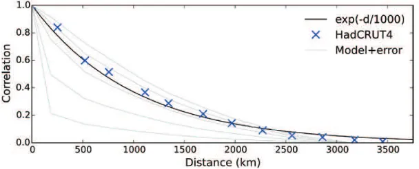
[image:7.536.118.422.480.603.2]The correlation between observations is inluenced both by the distance between the observations and by the noise in the individual observations. To isolate the effect of noise, correlograms were also determined for surface tempera-ture ields from the MERRA2 reanalysis (Gelaro et al., 2017), a recently developed atmospheric reanalysis spanning 1980 to the present. Figure 1 also shows how correlation changes with distance for the MERRA2 reanalysis data with
Figure 1. Correlation as a function of distance estimated from pairwise comparison of cells from the HadCRUT4 blended land/ ocean data. Crosses indicate binned averages. The thick line is the least squares it of an exponential function against every indi-vidual cell difference. Thin lines show the correlation with distance for the MERRA2 reanalysis with spatially constant geographical noise of 0.25°C (top line), 0.5°C, 1.0°C, 2.0°C and 5.0°C (bottom line).
D
o
w
n
lo
a
d
e
d
fro
m
h
ttp
s:
//a
ca
d
e
mi
c.
o
u
p
.co
m/
cl
ima
te
syst
e
m/
a
rt
icl
e
-a
b
st
ra
ct
/3
/1
/d
zy0
0
3
/5
0
5
6
4
3
4
b
y
U
n
ive
rsi
ty
o
f S
h
e
ffi
e
ld
u
se
r
o
n
1
0
O
ct
o
b
e
r
2
0
1
different amounts of geographically constant noise. When the noise signal is small, the correlogram has a bell curve shape. Increasing noise scales the correlations for all distances greater than zero, and so the it to the exponential model is somewhat contingent on the magnitude of the noise contribution. The observed correlogram falls between the reanalysis correlograms for a noise contribution of between 0.5°C and 1.0°C, consistent with estimates from Morice et al. (2012) for the size of this term in real world data.
The GTA1 method includes several simpliications which might impact the eficiency of the estimator. The method will, therefore, be tested by reconstructing temperature ields from incomplete and noisy data where the correct answer is known. The MERRA2 reanalysis was used for this purpose; however, the ERA-interim reanalysis (Dee et al., 2011), which shows faster Arctic warming over recent years (Simmons and Poli, 2015; Simmons et al., 2017), leads to similar conclusions.
The validation method follows a similar approach to that used in the estimation of coverage uncertainty in the HadCRUT family of temperature products (Jones et al., 1997; Brohan et al., 2006; Morice et al., 2012):
• The reanalysis 2m air temperature is converted to an air temperature anomaly using a 30-year baseline period and converted to the same grid as the observational record.
• A ‘true’ global mean surface temperature anomaly is calculated from the spatially complete reanalysis ield. • Coverage is reduced to match a month from the observational record, and random noise is added to each grid cell
in the reanalysis ield. A global mean surface temperature estimate is then constructed from the coverage reduced noisy data using the estimator to be tested. The root-mean-square (RMS) error between the estimate and the true value, evaluated using multiple months of data from the reanalysis, is used to evaluate the estimator.
Each month in the observational record produces a coverage mask. This mask is used in conjunction with the cor-responding month from every year in the reanalysis to produce an error estimate for a given estimator. For example, for the observational coverage from January 1940, the reanalysis ields for the 37 Januaries between 1980 and 2016 are used in estimating the errors. This assumes that the spatial scale of variability is invariant under transient climate change; this assumption will be tested later using a longer reanalysis.
The validation method is contingent on the use of realistic estimates of the noise to be added to each grid cell in the reanalysis data. While the HadCRUT4 dataset provides uncertainty estimates for each individual grid cell (Morice et al., 2012), these estimates do not include contributions from temporally and spatially correlated biases in the land and sea surface temperature observations, which are instead provided through an ensemble of reconstructions and covariance matrices (Kennedy et al., 2011; Morice et al., 2012).
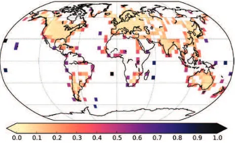
An independent estimate for the cell noise including all of the relevant contributions was, therefore, deter-mined from the temperature data themselves. A 3 × 3 block of grid cells was omitted from the map, and the value for the centre cell of the omitted region restored by kriging using the method of Cowtan and Way (2014). The error in the cell value was then estimated from the difference between the observed and reconstructed values. The calculation was repeated for each cell in turn. The RMS error for a given cell was then estimated from the RMS of the errors (over time) in that cell, for those cells with at least 60 months of differences over the period 1981–2010.
The errors in isolated Antarctic observations are overestimated because there are no nearby stations, and the noise estimate, therefore, contains a signiicant contribution from the geographical differences between stations. The max-imum value for the cell noise was, therefore, capped at the 99th percentile of the values obtained over the whole map, with the result that the inland Antarctic cells were given a similar error to cells in the Arctic. The resulting noise map is shown in Figure 2. For cells where insuficient data were available to estimate the error, RMS error values were extrapolated by kriging.
The noise estimates show a similar spatial pattern to uncorrelated error estimates from Morice et al. (2012)
for both land and ocean data but are about 50% larger in size: this relects the facts that some of the error sources identiied by Morice et al. are not included in the comparison, and that our estimates are inlated by interpolation error. Noise will be larger for earlier periods because there are often fewer observations per grid cell; however, when identifying climatic contributions to coverage, bias annual and decadal error estimates are more relevant than the monthly estimates used here. On this basis, the noise estimates are likely to be conservative for recent decades but may be underestimated for the early record. Our noise estimates do not include the effects of long range spatial correlated biases which are represented in the HadCRUT4 by an ensemble of temperature realizations, because while these
D
o
w
n
lo
a
d
e
d
fro
m
h
ttp
s:
//a
ca
d
e
mi
c.
o
u
p
.co
m/
cl
ima
te
syst
e
m/
a
rt
icl
e
-a
b
st
ra
ct
/3
/1
/d
zy0
0
3
/5
0
5
6
4
3
4
b
y
U
n
ive
rsi
ty
o
f S
h
e
ffi
e
ld
u
se
r
o
n
1
0
O
ct
o
b
e
r
2
0
1
contribute to the total uncertainty in the global mean temperature anomaly, they have comparatively little impact on the contribution of incomplete coverage to that uncertainty.
The noise map was used to add uncorrelated noise series to each cell in the reanalysis data from a normal distribu-tion with mean of zero and standard deviadistribu-tion equal to the estimated RMS error for that cell. This does not account for the partial correlation of the errors in the sea surface temperature data, which may lead to the impact of noise in the data being slightly underestimated.
To determine the optimum value of the length-scale d0, the errors in the GTA1 estimator were evaluated for length-scales in the range 500–1500 km. The RMS error in the GTA1 estimate as a function of length-scale is shown
in Figure 3. The results from reconstructing the reanalysis data support a value of between 800 and 900 km for d0,
similar to but slightly lower than the value determined from the observations.
The GTA1 method was then tested to ensure that the weighting of the data reduces to simple area weighting (i.e. Equation 2) in the case where the temperature ield is spatially complete. The weights given to grid cells as a function
of latitude are in good agreement between the two methods (Fig. 4). This result holds for values of the length-scale d0
[image:9.536.120.416.265.445.2]which are similar to or greater than the cell spacing: values of d0 which are signiicantly less than the cell spacing lead to cell weights which diverge from the cell areas, approaching uniform (i.e. non-area) weighting as d0 tends to zero. The equivalence to area weighting is also contingent on the use of the correlation matrix rather than the covariance matrix in Equation 5, otherwise regions with noisier observations are systematically downweighted.
[image:9.536.118.419.486.613.2]Figure 3. RMS error in global mean surface temperature estimates as a function of length-scale d0 for the GTA1 estimator. The error is evaluated by reducing the coverage of every year of the MERRA2 reanalysis data to match the coverage of the HadCRUT4 observations for the years 1981–2010.
Figure 2. RMS error in degree Celsius in the HadCRUT4 data estimated from the difference between the value of a cell and a value inferred from nearby (but non-neighbouring) cells by kriging. Data are for the period 1981–2010.
D
o
w
n
lo
a
d
e
d
fro
m
h
ttp
s:
//a
ca
d
e
mi
c.
o
u
p
.co
m/
cl
ima
te
syst
e
m/
a
rt
icl
e
-a
b
st
ra
ct
/3
/1
/d
zy0
0
3
/5
0
5
6
4
3
4
b
y
U
n
ive
rsi
ty
o
f S
h
e
ffi
e
ld
u
se
r
o
n
1
0
O
ct
o
b
e
r
2
0
1
Figure 4. Weights given to grid cells as a function of latitude in the case of a spatially complete ield by a simple weighted average based on cell area, and by the GTA1 estimator with e-folding radius d0 of 250 or 800 km.
Figure 5. RMS error in global mean surface temperature estimates as a function of coverage. The four estimators are compared on the basis of the error in reconstructing coverage reduced MERRA2 data, where coverage is determined by each of 12 months of a given year in the HadCRUT4 data.
4. Results
Four estimators were evaluated on the basis of their skill in reconstructing the global mean of the MERRA2 ields from the noise-added data using historical coverage masks:
1. The global mean of the observed cells, which is the method used in combination with different levels of inilling by Vose et al. (2012), Hansen et al. (2010) and Japan Meteorological Agency (2017).
2. The mean of the hemispheric means of the observed cells, which is the method used by Morice et al. (2012). 3. The mean of the zonal means, which has been used for radiosonde data by Thorne et al. (2005) and for surface
temperature data by Gleisner et al. (2015) under the assumption that temperature anomalies are primarily cor-related with other temperature anomalies at the same latitude.
4. The generalized least squares estimator GTA1 described by Equations 5 and 6, with the length-scale d0 set to 800 km.
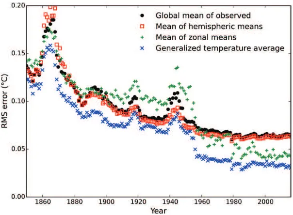
The RMS errors for the four different global mean estimators are plotted for the coverage of each month in the HadCRUT4 record in Figure 5. The global mean of the observed cells and the mean of the hemispheric means lead to very similar RMS errors, with the mean of the hemispheric means performing slightly better during the mid-20th century but worse during the 19th century. The mean of the zonal means performs substantially better than the global
D
o
w
n
lo
a
d
e
d
fro
m
h
ttp
s:
//a
ca
d
e
mi
c.
o
u
p
.co
m/
cl
ima
te
syst
e
m/
a
rt
icl
e
-a
b
st
ra
ct
/3
/1
/d
zy0
0
3
/5
0
5
6
4
3
4
b
y
U
n
ive
rsi
ty
o
f S
h
e
ffi
e
ld
u
se
r
o
n
1
0
O
ct
o
b
e
r
2
0
1
[image:10.536.118.420.407.629.2]or hemispheric means for the period since 1950; however, it performs worse than these methods prior to that date. The GTA1 estimator performs better than all the other estimators over the whole of the record, and in particular leads to RMS errors which are about half of the error from the global or hemispheric means for recent years. Since errors combine as variances, this implies that use of the GTA1 estimator mitigates three quarters of the error variance from sampling and measurement errors in the global or hemispheric means.
The difference between the generalized least squares average and the simple area weighted average may be under-stood by examining the weights given under the GTA1 approach to different cells, illustrated using the data from January 1920 of the CRUTEM4 land temperature dataset (Jones et al., 2012), normalized such that the largest weight is equal to one (Fig. 6). Isolated observations are given unit weight. Isolated pairs of adjacent observations are given just over half weight. Densely sampled observations are further downweighted inversely with the density of observa-tions, to produce an effective area weighting.
The weighting scheme serves to minimize the combined effect of sample noise (arising from there being insuficient observations) and sample bias (arising from some areas of the planet being over-represented)—the latter will be referred to as coverage error. When observations are sparse, all observations are given equal weight to minimize the impact of the error in any individual observation (i.e. assuming homoscedasticity). When observations are plentiful, observations are weighted in inverse proportion to the density of observations to avoid the over-representation of densely sampled regions. The large reduction in error after 1950 (Fig. 5) shows that coverage error is the dominant problem post-1950, and therefore downweighting the densely sampled regions leads to a better estimate of global mean temperature. This beneit is realized despite the fact that the errors are in reality heteroscedastic (Morice et al., 2012).
A theoretical estimate of the expected coverage error can be obtained from Equation 9. However, this estimate does not include the contribution of sample noise arising from errors in the observations, which is present even when coverage
is complete and so Var(T̂) is zero. The contribution of sample noise to the error in T̂ can be estimated using Equation
10 from the cell weights wGLS and the diagonal matrix Σ whose diagonal elements are the estimated noise variances for
each grid cell, determined empirically from the observations as described in Section 3 (Kagan, 1997, equation 3.1.5).
T w w
Varnoise( )= GLS Σ GLS (10)
The total error variance of the GTA1 estimator should be given by the sum of Var(T̂) and Var
noise(T̂). This estimate of
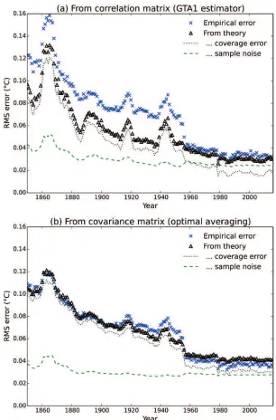
the uncertainty in the GTA1 estimator, along with the contributory terms, is compared to the empirical RMS error
in Figure 7a. The theoretical estimate of the uncertainty in the estimator agrees well with the empirical values for
the period from the late 1950s when Antarctic observations are available, but underestimates the uncertainty for the earlier periods, which suggests that the correlation model is too simple to produce optimal results for the early part of the record.
The correlation matrix C can be converted into a covariance matrix by multiplying each row and column by
[image:11.536.153.386.495.636.2]the standard deviations of the temperature anomalies for the corresponding grid cells. However, if the covariance matrix is used in Equation 5, the resulting weights do not tend towards the cell areas as coverage improves. Correct determination of the weights from the covariance matrix requires the more complex normalization procedure of
Figure 6. Weights given under the GTA1 approach to each grid cell for a map with the coverage of the CRUTEM4 data in January 1920, scaled such that the greatest weight is equal to 1. The weights are dimensionless.
D
o
w
n
lo
a
d
e
d
fro
m
h
ttp
s:
//a
ca
d
e
mi
c.
o
u
p
.co
m/
cl
ima
te
syst
e
m/
a
rt
icl
e
-a
b
st
ra
ct
/3
/1
/d
zy0
0
3
/5
0
5
6
4
3
4
b
y
U
n
ive
rsi
ty
o
f S
h
e
ffi
e
ld
u
se
r
o
n
1
0
O
ct
o
b
e
r
2
0
1
Kagan (1997, equation 3.3.7) or Weber and Madden (1995, equation 13) (the additional normalization has no effect if applied to the correlation matrix). Figure 7b shows the theoretical and empirical uncertainties estimates obtained when using the covariance matrix, which now show good agreement over the whole period. While performance of the correlation and covariance calculations is similar for recent decades, use of the covariance matrix noticeably reduces the errors in the early period. If coverage is poor and complexity is not an issue, the full optimal averaging method of Kagan should, therefore, be used in preference to the simpler GTA1 estimator.
Figure 7. Comparison of the theoretical and empirical estimates of RMS error in the temperature estimates as a function of cover-age. (a) Error contributions using the GTA1 estimator; (b) error contributions using the covariance matrix instead of the correlation matrix, with the appropriate normalization. The empirical estimate from Figure 5 is compared to the theoretical estimate from the sum in quadrature of Equations 9 and 10. The individual contributions of the coverage error and sample noise terms are also shown.
D
o
w
n
lo
a
d
e
d
fro
m
h
ttp
s:
//a
ca
d
e
mi
c.
o
u
p
.co
m/
cl
ima
te
syst
e
m/
a
rt
icl
e
-a
b
st
ra
ct
/3
/1
/d
zy0
0
3
/5
0
5
6
4
3
4
b
y
U
n
ive
rsi
ty
o
f S
h
e
ffi
e
ld
u
se
r
o
n
1
0
O
ct
o
b
e
r
2
0
1
The same approach can be used to analyse the errors for the other estimators by substituting the effective cell weights
for that estimator in place of wGLS. The coverage error and sample noise for the global mean of the observed cells and the
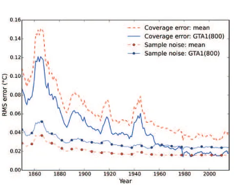
GTA1 estimator are shown in Figure 8. The GTA1 estimator reduces the coverage error compared to the global mean of the observed cells at a cost of increasing the sample noise. The coverage error is the dominant source of error for the global mean of the observed cells for the whole of the record, and so this provides a net reduction in the error of the estimator. Sample noise is minimized by using equal weights (or when allowing for heteroscedasticity by weighting according to the inverse variance for that grid cell), to avoid inlating the noise contribution of any individual observation. Coverage error is minimized by weighting the data to relect the true population. The improved performance of the GTA1 estimator over the global mean of the observed cells arises from a better compromise between these two sources of error.
In contrast to Kagan (1979), the noise contribution of individual cell values to the global mean is not handled explicitly in the GTA1 estimator, rather the global scale of the noise contribution is handled through the length-scale of the correlogram d0, although the it of the exponential model becomes poorer with lower or higher noise levels than those in the HadCRUT4 observations (Fig. 1). In the absence of noise, inclusion of an isolated cell observation reduces the uncertainty in the resulting global mean in proportion to the area of the planet for which that observation is informative, which is controlled by the length-scale. Since uncertainties sum in quadrature, they are dominated by the larger source of error, thus when the noise is less than the bias which is mitigated by including that cell, the cell noise has little effect on the correlogram. If the cell noise exceeds the bias mitigated by including that cell, the optimal range for the correlogram drops rapidly, with the effect that multiple observed cells are required to provide an inform-ative temperature estimate for the same area.
4.1. Contributions to coverage uncertainty
Coverage uncertainty in a global mean temperature estimate from spatially incomplete data arises from two sources:
changes in the temperature of the unobserved region relative to the observed region and changes in coverage. Let Tgl
be the true global mean surface temperature, Tobs be the mean temperature of the observed region, Tunobs be the mean
temperature of the unobserved region and funobs be the fraction of the surface which is unobserved, then:
= − +
Tgl Tobs(1 funobs) Tunobs unobsf . (11)
If the mean temperature is estimated from the average of the observed region alone, the error in the resulting
estimate will be ϵ = Tobs − Tgl. Let the difference between the means of the unobserved and observed regions be
Dunobs = Tobs − Tunobs, then:
=
[image:13.536.150.396.432.622.2] Dunobs unobsf . (12)
Figure 8. Comparison of the coverage error and sample noise contributions for both the global mean of the observed cells and the GTA1 estimators.
D
o
w
n
lo
a
d
e
d
fro
m
h
ttp
s:
//a
ca
d
e
mi
c.
o
u
p
.co
m/
cl
ima
te
syst
e
m/
a
rt
icl
e
-a
b
st
ra
ct
/3
/1
/d
zy0
0
3
/5
0
5
6
4
3
4
b
y
U
n
ive
rsi
ty
o
f S
h
e
ffi
e
ld
u
se
r
o
n
1
0
O
ct
o
b
e
r
2
0
1
When using temperature anomalies, the absolute value of the bias is irrelevant; however, changes in bias over time will lead to an error in temperature trends spanning the change in bias. The change in bias obeys a product rule:
≈ +
δ Dunobsδfunobs funobsδDunobs. (13)
Therefore, a change in coverage bias may arise from a change in the difference between the temperatures of observed
and unobserved regions, or from a change in coverage subject to Dunobs being non-zero.
Changes in Dunobs may be noise-like, for example due to weather systems moving into or out of the unobserved
region, or bias-like, for example due to relative changes in climate between the observed and unobserved regions rela-tive to the baseline period. The rapid warming of the incompletely observed Arctic is an example of the latter (Cowtan and Way, 2014), although decadal scale regional climate change due to internal variability has been shown to occur elsewhere as well (Xie et al., 2015).
To separate the effects of changes in climate and changes in coverage, additional validation tests were performed in which the coverage for a given month was used to calculate the error due to limited coverage in a historical reanalysis temperature ield for the corresponding month only. The ERA 20th Century Reanalysis (ERA20C) was used for this experiment (Poli et al., 2013) and provides a spatially complete temperature ield covering the period 1900–2010. The reanalysis is based on temperature, pressure and wind observations from the oceans, and pressure and wind observations from land weather stations. However, for unsampled regions (such as Antarctica in the early 20th century), the reanalysis temperatures are determined solely by the atmospheric model and boundary condi-tions and may also be impacted by observational biases. No noise was added to ERA20C reanalysis data.
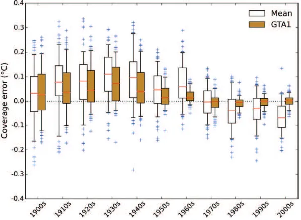
Figure 9 shows the decadal distributions of monthly temperature errors using either the global mean of the observed cells or the GTA1 estimator to reconstruct the mean of the ERA20C temperature ield using the observa-tional coverage from the years 1860, 1910, 1960 and 2010 for the corresponding month. With 1860 coverage, the range of errors is large for both the global mean and GTA1 estimators. With 1910 coverage, the GTA1 estimator tends to reduce the decadal bias and provides a slight reduction in the spread of the errors (in particular the outliers). With 1960 coverage, bias is substantially reduced and the spread of the errors reduced. With 2010 coverage, bias is almost eliminated and the spread of the errors substantially reduced.
Bias is expected to be lower during the 1961–90 baseline period because Dunobs should be close to zero, but in
practice only the 1970s temperature estimates show little bias when using the global mean estimator. The spread in the errors due to the weather contribution to coverage error is large compared to the persistent climatic contribution; however, there is a centennial trend from a warm to a cool bias in the global mean estimator for all coverages, and in the GTA1 estimator for 1860 and 1910 coverage due to the faster warming of the unobserved regions (Simmons et al., 2010). The global mean consistently underestimates the warming in the reanalysis data for any historical coverage. The GTA1 estimator provides a good estimate of the rate of warming for 1960 or 2010 coverage but underestimates the rate of warming when limited to 1860 or 1910 coverage.
Figure 10 shows the same experiment but using the historical coverage for the corresponding month as the basis for temperature reconstruction. For the period since the 1950s, bias is near zero and noise is dramatically reduced by the GTA1 estimator. For earlier decades, the GTA1 estimator provides a modest reduction in bias but little reduction in noise. The bias tends to be undercorrected suggesting that the GTA1 estimator is conservative with respect to the magnitude of the bias correction.
Changes in bias when using ixed coverage (Fig. 9) arise from changes in temperature anomaly in the unobserved region relative to the observed region, while the changes in bias when using historical coverage include the additional contribution from changes in coverage. The most notable change in the 1950s is the establishment of the Antarctic weather stations. The GTA1 estimator leads to consistently low noise and bias with 2010 coverage; however, it does not signiicantly reduce noise and only mitigates some bias with pre-1950 coverage. The actual bias estimates are, however, contingent on the reanalysis producing realistic temperatures in regions where no weather station observations are present.
4. 2. Impact of temperature estimators on the global warming ‘hiatus’
Numerous research papers have discussed a possible ‘hiatus’ in global warming at the start of the 21st century
(Lewandowsky et al., 2015; Medhaug et al., 2017). The IPCC Fifth Assessment Report noted a trend in the HadCRUT4
temperature record of 0.04°C/decade for the period 1998–2012 (Hartmann et al., 2013). This trend is substantially
D
o
w
n
lo
a
d
e
d
fro
m
h
ttp
s:
//a
ca
d
e
mi
c.
o
u
p
.co
m/
cl
ima
te
syst
e
m/
a
rt
icl
e
-a
b
st
ra
ct
/3
/1
/d
zy0
0
3
/5
0
5
6
4
3
4
b
y
U
n
ive
rsi
ty
o
f S
h
e
ffi
e
ld
u
se
r
o
n
1
0
O
ct
o
b
e
r
2
0
1
below the 32-year trend of about 0.17°C/decade (Foster and Rahmstorf, 2011) after removal of El Niño and other effects. Inilled temperature records from NASA and NOAA showed trends which were only slightly higher; however, these records did not at the time correct for a known bias due to the transition from ship to buoy measurements of sea surface temperature (Smith et al., 2008; Kennedy et al., 2011). The trend over the hiatus period is also inluenced by a residual uncorrected bias in the ship data (Huang et al., 2015; Hausfather et al., 2017), and a trend from El Niño to La Niña conditions over the period.
Figure 9. Error in the global mean of the observed cells and the GTA1 estimators of global mean surface temperature, grouped by decade when reconstructing months of the ERA20C reanalysis data reconstructed. Boxes show the interquartile range and whiskers the 5–95% range of errors for individual months in the decade. The line bisecting each box is the median, which provides an estimate of the decadal bias. The four panels show reconstructions using the HadCRUT4 observational coverage for the years 1860, 1910, 1960 and 2010.
D
o
w
n
lo
a
d
e
d
fro
m
h
ttp
s:
//a
ca
d
e
mi
c.
o
u
p
.co
m/
cl
ima
te
syst
e
m/
a
rt
icl
e
-a
b
st
ra
ct
/3
/1
/d
zy0
0
3
/5
0
5
6
4
3
4
b
y
U
n
ive
rsi
ty
o
f S
h
e
ffi
e
ld
u
se
r
o
n
1
0
O
ct
o
b
e
r
2
0
1
Temperature trends for HadCRUT4 version 4.1.1, which was the current version at the time of preparation of Hartmann et al., and for the now current version 4.6.0, were determined using the four estimators outlined earlier to determine the sensitivity of the trend to the temperature averaging method. The results are shown in Table 1.
The global mean of the observed cells and the mean of the hemispheric means both produce values consistent with Hartmann et al. (2013). The generalized least squares (GTA1) method produces a trend which is more than twice that of HadCRUT4.1.1 over the same period, while the mean of the zonal means method of Gleisner et al. (2015) produces an intermediate trend which is still closer to the GTA1 value. The use of the GTA1 method accounts for more than a third of the difference in trend between the hiatus period and the 32-year trend from Foster and Rahmstorf (2011). This increase in warming over the supposed hiatus period is also observed in records which use inilling to improve coverage (Cowtan and Way, 2014; Karl et al., 2015).
5. Discussion
[image:16.536.118.421.269.490.2]Historical temperature record products are utilized for multiple purposes, sometimes with conlicting requirements. Gridded temperature data are used to evaluate the performance of climate models and to identify spatial signatures associated with different climatic inluences. The gridded data are also summarized by a global mean surface tempera-ture estimate which may be used to quantify change in global climate for public and policy purposes, and to estimate climate sensitivity in simple energy balance calculations (e.g. Otto et al., 2013).
Table 1. Temperature trends in degree Celsius per decade for the period 1998–2012 (Hartmann et al., 2013) using the four
different estimators of global mean surface temperature
Method HadCRUT4.1.1 HadCRUT4.6.0
Global mean of observed cells 0.040 0.054
Mean of hemispheric means 0.040 0.052
Mean of zonal means 0.074 0.086
GTA1(800) 0.088 0.098
[image:16.536.55.481.563.633.2]Trends are given for the HadCRUT4.1.1 data, which were current at the time of Hartmann et al., and for the most recent version.
Figure 10. Error in the global mean of the observed cells and the GTA1 estimators of global mean surface temperature, grouped by decade when reconstructing months of the ERA20C reanalysis data reconstructed using the HadCRUT4 observational coverage from the corresponding year of the observational record.
D
o
w
n
lo
a
d
e
d
fro
m
h
ttp
s:
//a
ca
d
e
mi
c.
o
u
p
.co
m/
cl
ima
te
syst
e
m/
a
rt
icl
e
-a
b
st
ra
ct
/3
/1
/d
zy0
0
3
/5
0
5
6
4
3
4
b
y
U
n
ive
rsi
ty
o
f S
h
e
ffi
e
ld
u
se
r
o
n
1
0
O
ct
o
b
e
r
2
0
1
The HadCRUT4 record provides a monthly record of gridded temperature observations, with each observation contributing to only a single map grid cell. The Japan Meteorological Agency record (Japan Meteorological Agency, 2017) adopts a similar approach for land-based weather stations. In contrast, records from Hansen et al. (2010), Rohde et al. (2013) and Cowtan and Way (2014) use inilling to produce a temperature ield with near global cov-erage, which may be averaged by conventional methods. The errors in the resulting averages are contingent on the effectiveness of the inilling method.
The non-inilled temperature products have an important beneit for the evaluation of climate models. The gridded temperature record can be compared to the climate model outputs after reducing coverage to match the observational record. The beneit of using a non-inilled product in this case is that differences between the models and observations must arise from either the models or the observations. By contrast when using an inilled record, differences may arise from the models, the observations or from artefacts of the inilling method.
The simplicity of the gridded observational record leads to a product which is easier for temperature record users to understand, and if necessary to reproduce. Simple methods are easier to debug and maintain, which is important for products which must be maintained over many years by changing personnel. There are, therefore, multiple reasons to maintain non-inilled gridded observational records. A simple average of the resulting gridded data, however, can produce misleading results, with the temperature trends during the hiatus period being a notable example.
We have proposed a less biased estimator for determining the global mean surface temperature from spatially incomplete observations. For recent years, this estimator mitigates the larger part of the error associated with the use of the naive area weighted mean. The estimator is almost identical to the use of kriging to inill to global coverage and then averaging the resulting ield; however, it is simpler to implement and analyse. Implementation requires around 20 lines of computer code, and the results are determined solely by the temperature ield (including the coverage mask) and a single parameter which describes the range of spatial autocorrelation in the temperature ield. The estimator is also less biased than the mean of the zonal means which has been used with radiosonde data.
A number of more sophisticated approaches to averaging temperature data have been proposed, from Kagan (1979) to the recent works of Ilyas et al. (2017) and Huang et al. (2017). We do not intend the simple estima-tor proposed here to be a replacement for such methods; however, it does provide an easily understood and easily analyzed demonstration of why more naive averages are inadequate. Ideally, global temperature estima-tion would be performed using the optimal averaging method of Kagan or more modern methods; however, where simplicity of implementation and reproducibility are concerns, the GTA1 estimator can still substantially reduce the coverage error contribution to temperatures estimates for recent decades. The impact on temperature trends during the apparent ‘hiatus’ period provides an illustration of why good statistical estimators of global mean temperature are required for use in the evaluation of both historical temperature change and current temperature trends.
Supplementary material
Data and methods for this paper are available at https://doi.org/10.15124/c47f6da3-2430-4f0e-973e-6f6597c6da42 with updates at http://www-users.york.ac.uk/~kdc3/papers/coverage2018.
Supplementary material is available at Dynamics and Statistics of the Climate System online.
Declaration
Funding: PT was partially supported by the Copernicus Climate Change Service under C3S 311a Lot 2 (Global Land and Marine Observations Database) activities. RW was partially supported by the EPSRC-funded Past Earth Network (grant number EP/ M008363/1).
Ethical approval: none. Conlict of interest: none.
Acknowledgements
Two reviewers provided insightful suggestions which improved the manuscript.
D
o
w
n
lo
a
d
e
d
fro
m
h
ttp
s:
//a
ca
d
e
mi
c.
o
u
p
.co
m/
cl
ima
te
syst
e
m/
a
rt
icl
e
-a
b
st
ra
ct
/3
/1
/d
zy0
0
3
/5
0
5
6
4
3
4
b
y
U
n
ive
rsi
ty
o
f S
h
e
ffi
e
ld
u
se
r
o
n
1
0
O
ct
o
b
e
r
2
0
1