Advance Access publication 2018 February 20
A comparison of shock–cloud and wind–cloud interactions: effect of
increased cloud density contrast on cloud evolution
K. J. A. Goldsmith
‹and J. M. Pittard
School of Physics and Astronomy, University of Leeds, Woodhouse Lane, Leeds LS2 9JT, UK
Accepted 2018 February 6. Received 2018 January 19; in original form 2017 July 10
A B S T R A C T
The similarities, or otherwise, of a shock or wind interacting with a cloud of density contrast
χ=10 were explored in a previous paper. Here, we investigate such interactions with clouds of higher density contrast. We compare the adiabatic hydrodynamic interaction of a Mach 10 shock with a spherical cloud ofχ=103with that of a cloud embedded in a wind with identical
parameters to the post-shock flow. We find that initially there are only minor morphological differences between the shock–cloud and wind–cloud interactions, compared to whenχ=10. However, once the transmitted shock exits the cloud, the development of a turbulent wake and fragmentation of the cloud differs between the two simulations. On increasing the wind Mach number, we note the development of a thin, smooth tail of cloud material, which is then disrupted by the fragmentation of the cloud core and subsequent ‘mass-loading’ of the flow. We find that the normalized cloud mixing time (tmix) is shorter at higherχ. However, a strong
Mach number dependence ontmixand the normalized cloud drag time,tdrag , is not observed.
Mach-number-dependent values oftmix andtdrag from comparable shock–cloud interactions
converge towards the Mach-number-independent time-scales of the wind–cloud simulations. We find that high χ clouds can be accelerated up to 80–90 per cent of the wind velocity and travel large distances before being significantly mixed. However, complete mixing is not achieved in our simulations and at late times the flow remains perturbed.
Key words: hydrodynamics – shock waves – stars: winds, outflows – ISM: clouds – ISM: kinematics and dynamics.
1 I N T R O D U C T I O N
The interstellar medium (ISM) is a dynamic entity, the study of which can allow insights into the nature of the ISM itself (see e.g. Elmegreen & Scalo2004; Mac Low & Klessen2004; Scalo & Elmegreen2004; McKee & Ostriker2007; Hennebelle & Falgarone
2012; Padoan et al.2014), as well as processes such as the formation of filamentary structures that are prevalent throughout the ISM. The interaction of hot, high-velocity, tenuous flows (e.g. shocks and winds) with much cooler, dense clumps of material (i.e. clouds), shapes and evolves these clouds and, ultimately, destroys them. A review of shock–cloud studies is presented in Pittard & Parkin (2016), whilst an equivalent review of wind–cloud studies can be found in Goldsmith & Pittard (2017).
Under certain circumstances, flows interacting with clouds can lead to the formation of tail-like morphologies or filamentary struc-tures. Observations have shown these to occur from the small scale, such as comet plasma tails (e.g. Brandt & Snow2000; Buffington
E-mail:[email protected]
et al.2008; Yagi et al.2015) to much larger scales, e.g. Hα-emitting filaments occurring within galaxies. Tails have been observed in NGC 7293 in the Helix nebula (O’Dell et al.2005; Hora et al.2006; Matsuura et al.2007, 2009; Meaburn & Boumis2010) (see also Dyson et al.2006for a corresponding numerical study) and also in the Orion Molecular Cloud OMC1 (Allen & Burton1993; Schultz et al.1999; Tedds et al. 1999; Kaifu et al. 2000; Lee & Burton
2000). Tail-like structures have also been found in galactic winds (Cecil et al.2001,2002; Ohyama et al.2002; Crawford et al.2005; McClure-Griffiths et al.2012,2013; Shafi et al.2015).
Numerical shock/wind–cloud studies which have had either a par-ticular focus on, or have noted, the formation of tails include Strick-land & Stevens (2000), Cooper et al. (2008), Cooper et al. (2009), Pittard et al. (2009), Pittard et al. (2010), and Banda-Barrag´an et al. (2016), whilst Pittard (2011) investigated the formation of tails in shell–cloud interactions. Pittard et al. (2009, 2010), for example, noted the formation of tail-like structures in 2D shock– cloud interactions where the cloud had a density contrastχ=103
and a high shock Mach number and suggested that this was be-cause the stripping of material was more effective at higher Mach numbers due to the faster growth of Kelvin–Helmholtz (KH) and
C
Rayleigh–Taylor (RT) instabilities. They found that well-defined tails formed only for density contrastsχ103, but developed for
a variety of Mach numbers.
In contrast, whilst there are a large number of wind–cloud simula-tions in the literature, very few have considered clouds with density contrasts of 103or greater. Those that have (e.g. Murray et al.1993;
Schiano et al. 1995; Vieser & Hensler 2007; Cooper et al.2009; Scannapieco & Br¨uggen2015; Banda-Barrag´an et al.2016) have tended not to vary the wind Mach number. Banda-Barrag´an et al. (2016), for example, noted the realistic nature of higher cloud den-sity contrasts (i.e.χ >100) but limited their adiabatic calculations to winds of Mach number 4.
In Goldsmith & Pittard (2017, hereafterPaper I), we compared shock-cloud and wind–cloud simulations using similar flow param-eters for a cloud density contrastχ =10, and explored the effect of increasing the wind Mach number on the evolution of the cloud. In that study, we found there to be significant differences between shock-cloud and wind–cloud interactions in terms of the nature of the shock driven through the cloud and the axial compression of the cloud, and noted that the cloud mixing time normalized to its crush-ing time-scale increased for increascrush-ing wind Mach number until it reached a plateau due to Mach scaling. In addition, we also found that clouds in high Mach number winds were capable of surviving for longer and travelling considerable distances. In the current pa-per, we extend our investigation to clouds with a density contrast higher than that of the first paper (χ = 103) and again compare
between simulations where the wind Mach number is varied. We also make comparisons between the current work andPaper I.
The outline of this paper is as follows: in Section 2 we introduce the numerical method and describe the initial conditions, whilst in Section 3 we present our results. Section 4 provides a summary of our results and our conclusions.
2 T H E N U M E R I C A L S E T- U P
The calculations in this study were performed on a 2DRZ axisym-metric grid using theMGadaptive mesh refinement hydrodynamical
code, where refinement and de-refinement are performed on a cell-by-cell basis (seePaper Ifor a detailed description of the refinement process).MGsolves the Eulerian equations of hydrodynamics, the full set of which can be found inPaper I. The code uses piecewise linear cell interpolation to solve the Riemann problem at each cell interface in order to determine the conserved fluxes for the time update. The scheme is second-order accurate in space and time and uses a linear solver in most instances (Falle1991).
The effective resolution is quoted as that of the finest grid,Rcr,
where ‘cr’ denotes the number of cells per cloud radius on the finest grid. All simulations were performed at a resolution ofR128, which
has been found to be the minimum necessary for key features in the flow to be adequately resolved and for the morphology and global statistical values to begin to show convergence (e.g. Klein et al.1994; Niederhaus2007; Pittard et al.2009; Pittard & Parkin
2016). As before, we measure all length scales in units of the cloud radius,rc, whererc=1, whilst velocities are measured in terms of
the shock speed through the background medium,vb(vb=13.6,
in computational units). Measurements of the density are given in terms of the density of the background medium,ρamb. The numerical
domain is set to be large enough so that the main features of the interaction occur before cloud material reaches the edge of the grid. Table1details the grid extent for each of the simulations.
[image:2.595.307.546.102.175.2]We make the following assumptions in order to maintain simplic-ity: the cloud is adiabatic (withγ=5/3) and we ignore the effects
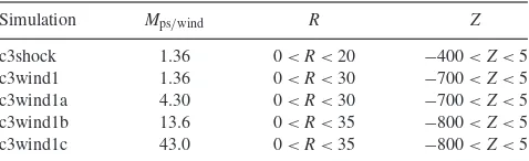
Table 1. The grid extent for each of the simulations presented in this paper (see Section 3 for the model naming convention).Mps/wind denotes the
effective Mach number of the post-shock flow/wind. Length is measured in units of the initial cloud radius,rc.
Simulation Mps/wind R Z
c3shock 1.36 0<R<20 −400<Z<5 c3wind1 1.36 0<R<30 −700<Z<5 c3wind1a 4.30 0<R<30 −700<Z<5 c3wind1b 13.6 0<R<35 −800<Z<5 c3wind1c 43.0 0<R<35 −800<Z<5
of thermal conduction, magnetic fields, self-gravity, and radiative cooling. Our assumption of adiabacity is consistent with the small-cloud-limit, whereby the cloud-crushing time-scale is much shorter than the cooling time-scale (cf. Klein et al.1994). Non-radiative interactions between shocks/winds and clouds are expected in the ISM (McKee & Cowie1975). We further justify our simplified set-up by noting that our primary goal is to provide an initial com-parison of shock–cloud and wind–cloud simulations and the simi-larities/differences between the two types of interaction are better isolated without the introduction of additional processes. We do not, therefore, concern ourselves at this stage with the detail of the processes which led to the cloud being embedded in the wind, nor with the effects of additional processes (e.g. radiative cooling) on the interaction. It should, however, be noted that 3D calcula-tions are necessary in future work and that they are expected to produce slightly different morphologies and statistical values once non-axisymmetric instabilities become important at late times (e.g. t> 5tcc Pittard & Parkin2016). More realistic 3D comparative
studies that include radiative cooling should be considered in the future.
2.1 The shock–cloud model
Our reference simulation is the shock–cloud modelc3shock(see Section 3 for the model naming convention). The simulated cloud is an idealized sphere and is assumed to have sharp edges (see e.g. Nakamura et al.2006; Pittard & Parkin2016for a discussion of how cloud density profiles affect the formation of hydrodynamic instabilities), in contrast to previous shock–cloud studies that used a soft edge to the cloud (e.g. Pittard & Parkin2016), and is initially in pressure equilibrium with the surrounding stationary ambient medium. The simulations are described by the shock Mach number, Mshock = 10, and the density contrast between the cloud and the
stationary ambient medium,χ=103. The shock–cloud simulation
begins with the shock initially located atz=1 (the shock propagates in the negativezdirection) and the cloud centred on the grid origin r, z=(0, 0).
The post-shock1density, pressure, and velocity for the shock–
cloud case relative to the pre-shock ambient values and to the shock speed areρps/wind/ρamb =3.9,Pps/wind/Pamb= 124.8, and
vps/wind/vb=0.74, respectively.
2.2 The wind–cloud model
In order to simulate a wind–cloud interaction, we begin by removing the initial shock and fill the domain external to the cloud with the
1We use the subscript ps/wind to denote quantities related to either the
same post-shock flow properties. At the start of the simulation, the cloud is instantly surrounded by a wind of uniform speed and direction, in line with previous wind–cloud studies (e.g. Banda-Barrag´an et al.2016). Since this is an idealized scenario as a first step towards more realistic simulations, we simplify the initialization of the wind and make the following assumptions: (a) the wind is associated with the post-shock flow properties of the shock–cloud model (i.e. we simulate a mildly supersonic wind using exactly the same post-shock flow conditions as used in the shock–cloud model) and (b) that it completely surrounds the cloud at time zero. Our aim is to provide comparable initial conditions for both interactions before any of the wind parameters are changed. This means that the cloud is initially underpressured compared to the wind. Astrophysically, this implies that the wind switches on rapidly.
Although the initial cloud density is the same in both the shock– cloud and wind–cloud simulations, the density contrast between the cloud and thewindin the latter case (χ) is given by factoring off the value of the post-shock density jump from the value ofχ, i.e.
χ=χ/3.9 (see Section 2.1).
In addition to the parameters described in Section 2.1, the wind– cloud simulations are also described by the effective Mach number of the wind,Mps/wind, given by
Mps/wind=
vps/wind
cps/wind
, (1)
wherecps/wind=
γPps/wind
ρps/wind is the adiabatic sound speed of the
post-shock flow/wind. For our initial wind–cloud simulation (model c3wind1),Mps/wind=1.36. Since the initial, unshocked cloud
pres-sure is equal toPamb, andPambPps/wind, the cloud does not start off
in pressure equilibrium with the wind and is thus underpressured with respect to the flow. Over the course of one cloud-crushing time-scale the cloud pressure increases until it is equal to or slightly greater than the pressure of the surrounding wind. It should be noted that the wind can travel a long way in the ‘cloud-crushing time’ due to the high density contrast of the cloud. This is a different set-up to other wind–cloud studies (e.g. Schiano et al.1995) where the sim-ulations begin with the cloud already in approximate ram pressure equilibrium with the wind, but is necessary in order to allow a more direct comparison to our shock–cloud simulation.
The value of the wind velocity,vps/wind, is given in Section 2.1.
In order to explore the effect of an increasing Mach number on the interaction, the velocity of the flow,vps/wind, is increased by factors
of√10,√100, and√1000 in order to increaseMps/wind. Values of
the wind Mach number are given in Table1.
2.3 Global quantities
The evolution of the cloud can be monitored through various in-tegrated quantities (see Klein et al.1994; Nakamura et al.2006; Pittard et al.2009; Pittard & Parkin 2016; Goldsmith & Pittard
2017). These include the core mass of the cloud (mcore), mean
ve-locity in thezdirection (vz, cloud), and cloud centre of mass in the
zdirection (zcloud). In addition, the morphology of the cloud can
be described by the effective radii of the cloud in the radial (a) and axial (c) directions, defined as
a=
5 2r
2
1/2
, c=[5(z2 − z2)]1/2, (2)
in addition to their ratio.
We use an advected scalar,κ, to trace the evolution of the cloud in the flow and distinguish between the cloud core and the
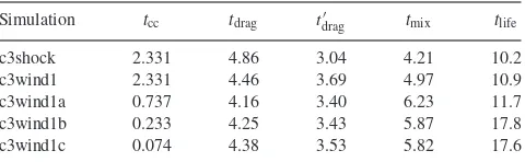
am-Table 2. A summary of the cloud-crushing time,tcc, and key time-scales,
in units oftcc, for the simulations investigated in this work. Note that the
value fortdraggiven here is calculated using the definition given in §2.3,
whilsttdrag is the time whenvz, cloud =vps/e, wherevpsis the post-shock
(or wind) speed in the frame of the unshocked cloud.
Simulation tcc tdrag tdrag tmix tlife
c3shock 2.331 4.86 3.04 4.21 10.2
c3wind1 2.331 4.46 3.69 4.97 10.9
c3wind1a 0.737 4.16 3.40 6.23 11.7
c3wind1b 0.233 4.25 3.43 5.87 17.8
c3wind1c 0.074 4.38 3.53 5.82 17.6
bient background. Therefore, we are able to compute each of the global quantities for either the cloud core and associated fragments (using the subscript ‘core’) or the entire cloud plus regions where cloud material is mixed into the surrounding flow (using the sub-script ‘cloud’). Motion is defined with respect to the direction of shock/wind propagation along thez-axis, with motion in that di-rection being termed ‘axial’ and motion perpendicular to that as ‘radial’.
2.4 Time-scales
We use the ‘cloud-crushing time’ given by Klein et al. (1994) for the initial shock–cloud simulation:
tcc=
√χ r
c
vb
. (3)
For the wind–cloud simulations, this time-scale is redefined accord-ing to the post-shock flow/wind velocity:
tcc=
C√χ rc
vps/wind
, (4)
where the constant C is given by the ratio of the post-shock flow/wind velocity to the velocity of the shock through the un-shocked medium,vps/wind/vb. The value of the constant depends on
the value of the shock Mach number (Mshock=10 in this work) used
in the shock–cloud simulation, against which the wind simulations are compared. Thus, for our initial shock and wind simulations, modelsc3shockandc3wind1, the value ofC=0.74 and is spe-cific to this Mach number and our adopted value ofγ. The value ofCis also dependent on the value ofvps/windwhich, in our later
wind–cloud models, is varied, resulting in differing values ofC. Therefore, tcc also varies depending on the particular simulation
under consideration. Values for the cloud-crushing time-scale for each simulation are given in Table2.
Several other time-scales are used, including the ‘drag time’,tdrag;
the ‘mixing time’,tmix, and the cloud ‘lifetime’,tlife (seePaper I
for a more detailed description of these time-scales). In all of the following our time-scales are normalized totcc. Time zero in our
calculations is defined as the time at which the intercloud shock is level with the leading edge of the cloud in the shock–cloud case. In the wind–cloud case, the simulation begins with the cloud already surrounded by the flow.
3 R E S U LT S
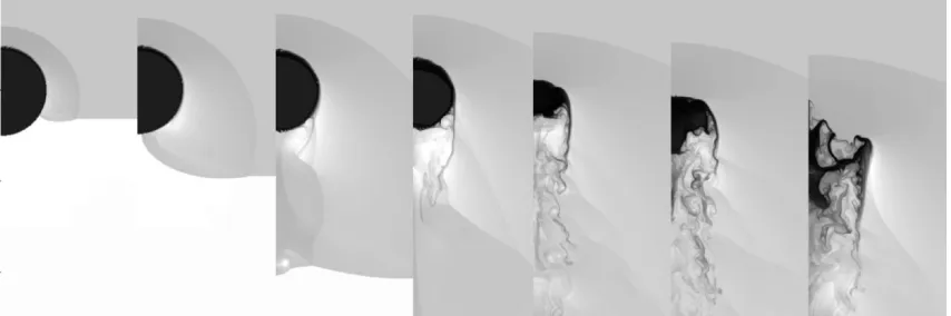
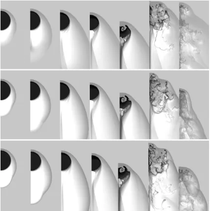
[image:3.595.310.550.112.186.2]Figure 1. The time evolution of the logarithmic density for modelc3shock. The grey-scale shows the logarithm of the mass density, from white (lowest density) to black (highest density). The density in this and subsequent figures has been scaled with respect to the ambient density, so that a value of 0 represents the value ofρamband 1 represents 10×ρamb. The density scale used for this figure extends from 0 to 3.8. The evolution proceeds left to right witht=0.043tcc,
t=0.084tcc,t=0.16tcc,t=0.31tcc,t=1.2tcc,t=2.0tcc, andt=3.6tcc. Ther-axis (plotted horizontally) extends 3rcoff-axis. All frames show the same
region (−5<z<2, in units ofrc) so that the motion of the cloud is clear. Note that in this and similar figures thez-axis is plotted vertically, with positive
towards the top and negative towards the bottom.
interaction when the Mach number of the wind is increased (models c3wind1atoc3wind1c).
At the end of this section we explore the impact of the interaction on various global quantities. InPaper I, we used a naming con-vention such that the higher velocity wind–cloud simulations were described from ‘wind1a’ to ‘wind1c’. Thus, in order to compare between the two papers we retain a similar naming convention such thatc3shockrefers to a shock–cloud simulation withχ=103. The
‘1a’ in modelc3wind1a, for example, indicates that the interaction has an increased wind Mach number compared to modelc3wind1.
3.1 Shock–cloud interaction
Fig.1shows plots of the logarithmic density as a function of time for model c3shock. The evolution of the cloud broadly proceeds as per modelc1shockinPaper I(whereMshock=10 andχ =10)
in that the cloud is initially struck on its leading edge, causing a shock to be transmitted through the cloud whilst the external shock sweeps around the cloud edge, and a bow shock is formed ahead of the leading edge of the cloud. There are a number of differences between the two models, as detailed below.
The rate at which the transmitted shock progresses through the cloud is considerably slower than the comparable simulation in
Paper I; in that paper, the shock was also much flatter whereas modelc3shockhas a semiflat shock, the end of which curves around the cloud flank (see the fourth panel of Fig. 1). The slowness of the transmitted shock and its progress through the cloud in the current simulation is attributed to the increased density of the cloud compared to modelc1shock.
Initially, the slow progress of the transmitted shock through the cloud means that the cloud appears to undergo little immediate compression in either the axial or radial directions, in contrast to the cloud inPaper I, which was flattened into an oblate spheroid even as the external shock was sweeping around the outside. However, when this is measured in units oftcc, maximum compression of the
cloud in the axial direction takes place byt1tcc(cf. panels 4 and
5 of Fig.1).
The surface of the cloud in the current simulation from the outset is not smooth (compared to the cloud edge in e.g. Pittard et al.
2009,2010; Pittard & Parkin2016). The rapid development of such
small instabilities is attributed to the fact that we used a sharp edge to our cloud (see Pittard & Parkin2016for a discussion of how soft cloud edges can hinder the growth of KH instabilities). It is also notable that the cloud moves downstream at a slightly slower rate than would be expected in comparison with previous inviscid shock–cloud calculations (cf. fig. 4 in Pittard et al.2009). This difference is likely to be due to the smooth edge given to the cloud in e.g. Pittard et al. (2009) which results in the cloud having slightly less mass than in our model.
The third panel of Fig.1shows that the external shock has reached ther=0 axis and cloud material is being ablated from the back of the cloud into the flow. The sheer across the surface of the cloud induces the growth of instabilities, leading to a thin layer of material being drawn away from the side of the cloud and funnelled downstream. At this point, the transmitted shock is still progressing through the cloud. With the transmitted shock curving around the edge of the cloud and also moving in from the rear, the cloud begins to exhibit a shell-like morphology, with a shocked denser outer layer encompassing the unshocked interior. This is a relatively short-lived morphology, since byt =1.2tcc the shocked parts of the cloud
collapse into each other, and the transmitted shock has exited the cloud and accelerated downstream. Cloud material is then ablated by the flow and expands supersonically downstream, forming a long and turbulent wake. The cloud core, however, remains relatively intact after the formation of the turbulent wake and persists for some time as a distinct clump (untilt≈5.2tcc, when it starts to
become more elongated and drawn-out along the axial direction). This behaviour differs from theχ=10 cloud investigated inPaper I, where the cloud was destroyed much more rapidly. However, it is in better agreement with inviscid simulations presented in Pittard et al. (2009), who showed that clouds withχ =103and a shock
Mach number of 10 form a turbulent wake, and that the mass loss at later times resembles a a single tail-like structure (see figs 4 and 7 of that paper).
3.2 Wind–cloud interaction
3.2.1 Comparison of wind–cloud and shock–cloud interactions
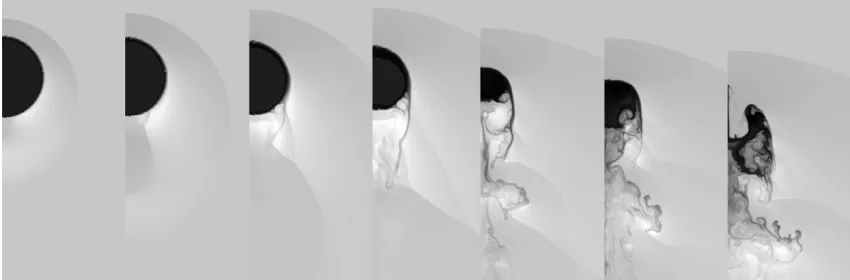
Figure 2. The time evolution of the logarithmic density for modelc3wind1. The grey-scale shows the logarithm of the mass density, scaled with respect to the ambient medium. The density scale used in this figure extends from 0 to 3.8. The evolution proceeds left to right witht=0.042tcc,t=0.077tcc,t=0.15tcc,
t=0.30tcc,t=1.2tcc,t=2.0tcc, andt=3.6tcc. All frames show the same region (−5<z<2, 0<r<3, in units ofrc) so that the motion of the cloud is
clear.
wind density, pressure, and velocity values are exactly the same as the post-shock flow values in modelc3shock.
As with modelsc1shockandc1wind1 inPaper I,c3shockand c3wind1 show broad similarities (cf. Figs 1and2). Both clouds have very similar morphologies and there is little to tell them apart, at least initially. However, there are subtle differences between the two models once the initial shock has progressed around the edge of the cloud. For example, the RT instability that develops on the cloud’s leading edge behaves differently to that in modelc3shock. This is due to an area of very low pressure in the shock–cloud case that is situated at the outside (right hand) edge of the ‘finger’ of cloud material forming due to the RT instability. This low-pressure area is absent in the wind–cloud case. This means that the RT finger is channelled more upstream in the wind–cloud model but expands more radially in the shock–cloud model (see the last 3 panels in Figs1and2). Furthermore, the flow past the cloud in the wind–cloud case is reasonably uniform, whereas that in the shock–cloud case sweeps around the RT finger and helps to push cloud material outwards in the radial direction. This means that the transverse radius of the cloud grows more quickly in model c3shockcompared toc3wind1 (see the final panel in Figs1and2, and also4e). However, in modelc3shockthe transverse radius of the cloud does not grow any further aftert=3.6tcc, whereas in model
c3wind1 it continues to do so and byt=5tccit is greater than in
modelc3shock. The continued lateral growth of the cloud in model c3wind1 coincides with a greater fragmentation of the core and a more rapid reduction in core mass, so that betweent=5 and 8tcc
the core mass inc3wind1 is less than that inc3shock(see Fig.4a). Once the transmitted shock has exited the cloud, the cloud in modelc3wind1 develops a long, low-density, turbulent wake similar to that in modelc3shock(but much less dense) in the downstream direction.2Unlike the cloud in modelc3shock, the cloud core in
modelc3wind1 is not drawn out along thezdirection, and once the core fragments the turbulent wake is disrupted by mass-loading of the core into the flow (not shown).
2At late times an axial artefact develops in modelsc3shockandc3wind1.
This is visible in the final panels of Figs1and2and is seen protruding upstream. Such artefacts are sometimes seen in 2D axisymmetric simulations and occur purely due to the nature of the scheme (fluid can become ‘stuck’ against the boundary). However, it does not appear to influence the rest of the flow and can be safely ignored in our work.
In comparison to modelc1wind1 inPaper I, the RT instability in modelc3wind1 expands upstream as opposed to the radial direction. This effect is caused by shock waves moving through the cloud, once the transmitted shocks from the front and rear of the cloud cross each other. Another difference between ourc3wind1 simulation and thec1wind1 simulation inPaper Iis that the rear edge of the cloud is not forced upwards to the same extent due to the action of shocks driven into the back of the cloud (cf. the second panel of Fig.2at t=0.077tccwith the second panel of Fig.2inPaper Iatt=0.82tcc).
A turbulent wake is not seen in modelc1wind1 inPaper I. The evolution of the cloud in modelc3wind1 bears some sim-ilarities to the adiabatic spherical cloud in the wind–cloud study by Cooper et al. (2009), where mass is immediately ablated from the back of the cloud in the form of a long sheet of material and moves downstream in a thin, turbulent tail (see the left-hand panels of fig. 7 in Cooper et al. (2009) showing the logarithmic density of the cloud, in aMwind =4.6 andχ=910 simulation). Their cloud
showed a large expansion in the transverse direction, with cloud material being torn away from the core in all directions and mixed in with the flow, i.e. comparable behaviour to our modelc3wind1. Such fragmentation of the cloud core is dissimilar to the evolution of the cloud in modelc3shock.
3.2.2 Effect of increasing Mwindon the evolution
Compared to modelc3wind1, models c3wind1a, c3wind1b, and c3wind1cdisplay a long-lasting and supersonically expanding cav-ity located to the rear of the cloud (similar to the higher wind Mach number simulations inPaper I) and a reduced stand-off distance between the cloud and the bow shock; these features are due to the increase in wind velocity and Mach number in these models.
There is much greater pressure at the leading edge of the cloud in the higherMwindsimulations. The density jump at the bow shock
in the higherMwind simulations is also greater, and the stand-off
distance between the bow shock and the leading edge of the cloud smaller, than in modelc3wind1. The greater compression at the bow shock reduces the flow velocity (normalized tovps/wind) around
the edge of the cloud, leading to a reduction in the growth rate of instabilities and decreased stripping of cloud material from the side of the cloud (when time is normalized totcc). The evolution of the
cloud in the higherMwindsimulations, therefore, is different to that
Figure 3. The time evolution of the logarithmic density for modelsc3wind1a(top row),c3wind1b(middle row), andc3wind1c(bottom row). The grey-scale shows the logarithm of the mass density, scaled with respect to the ambient medium. The density scale used in this figure extends from 0 to 3.8. The evolution proceeds left to right witht=0.07tcc,t=0.13tcc,t=0.25tcc,t=0.49tcc,t=1.84tcc,t=3.10tcc, andt=5.53tcc. The first five frames in each set show
the same region (−5<z<2, 0<r<3, in units ofrc) so that the motion of the cloud is clear. The displayed region is shifted in the sixth frame of each set
(−13<z<−1, 0<r<5) and the last frame (−23<z<−11, 0<r<5) in order to follow the cloud. similar morphologies, at least until aroundt≈1.8tcc. This is due to
the presence of the highly supersonic cavity (as opposed to the area of low pressure behind the cloud in modelc3wind1) which alters the way the wind flows around the cloud flanks. Instead of being focused on ther=0 axis immediately behind the cloud as in model c3wind1, the flow is deflected further downstream away from the cloud edge leading to a much lower pressure jump behind the cloud and restricting secondary shocks from being driven into the rear of the cloud. Thus, there is less turbulent stripping of cloud material from the rear of the cloud in these simulations compared to model c3wind1.
Interestingly, these high-Mwindmodels initially form a thin,
com-pressed, smooth tail of material ablated from the side and rear of the cloud (see panels 2, 3, and 4, corresponding tot=0.13, 0.25 and 0.49tcc, in each set of Fig.3), whereas, as already noted, the cloud
in modelc3wind1 forms instead a low-density turbulent wake. The
cause of this is the way the flow moves around the cloud edge. In modelc3wind1, the wind flows much closer to the cloud all the way around its edge. However, in modelc3wind1athe stronger bow shock deflects some of the flow away from the cloud edge, whilst the cavity serves to restrict the flow immediately behind the cloud. Thus, there is a slower removal of material from the cloud in the latter case. In addition, in modelc3wind1a, the flow converges on ther=0 axis, which serves to focus cloud material at this point, whereas in modelc3wind1 the flow changes direction and pushes upwards into the rear of the cloud. There is much less focusing of cloud material on ther=0 axis in this case and, thus, the tail of cloud material is much broader. This behaviour also differs from the comparable models inPaper I.
0 0.2 0.4 0.6 0.8 1 1.2
0 10 20 30
(a)
(b)
(c)
(d)
(e)
(f)
mcore
(m
c
)
Time (tcc)
c3shock c3wind1 c3wind1a c3wind1b c3wind1c
0 0.2 0.4 0.6 0.8 1 1.2
0 10 20 30
<v
z,cloud
> (v
ps/wind
)
Time (tcc)
c3shock c3wind1 c3wind1a c3wind1b c3wind1c
0 100 200 300 400 500
0 10 20 30
<z
cloud
> (r
c
)
Time (tcc)
c3shock c3wind1 c3wind1a c3wind1b c3wind1c
0 5 10 15 20 25 30 35
0 10 20 30
ccloud /acloud
Time (tcc)
c3shock c3wind1 c3wind1a c3wind1b c3wind1c
0 5 10 15 20
0 10 20 30
acloud
(r
c
)
Time (tcc)
c3shock c3wind1 c3wind1a c3wind1b c3wind1c
0 50 100 150 200
0 10 20 30
ccloud (rc
)
Time (tcc)
[image:7.595.80.517.61.524.2]c3shock c3wind1 c3wind1a c3wind1b c3wind1c
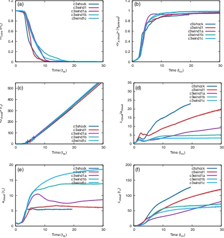
Figure 4. Time evolution of (a) the core mass of the cloud,mcore, (b) the mean velocity of the cloud in thezdirection,vz, (c) the centre of mass in the axial
direction,z, (d) the ratio of cloud shape in the axial and transverse directions,ccloud/acloud, (e) the effective transverse radius of the cloud,acloud, and (f) the
effective axial radius of the cloudccloud. Note that panel (c) shows the position of the centre of mass of each cloud att=tmix(indicated by the respectively
coloured crosses). In addition, the behaviour of the cloud in modelc3shockaftert≈20tcchas not been included in any of the above panels since the cloud
material drops below theβ=2/χthreshold at late times (see Section 2.2).
much further in the axial direction than that in modelc3wind1a(cf. the final panel in each set).
3.3 Statistics
We now explore the evolution of various global quantities of the interaction for both the shock–cloud and wind–cloud models. Fig.4
shows the time evolution of these key quantities, whilst Table2lists various time-scales taken from these simulations.
Fig.4(a) shows the time evolution of the core mass of the cloud in each of the simulations. It can be seen that modelsc3shock andc3wind1 are closer in their behaviour than either of them is
to the higher wind Mach number simulations (which, however, are more closely converged to each other as expected from Mach scaling considerations). The cloud core in modelc3shock drops to 50 per cent of its initial value more quickly than that of model c3wind1 due to the faster transverse expansion of the cloud in the former case. However, the greater lateral expansion of the cloud in modelc3wind1 at later times, and hence its greater effective cross-section, means that it then loses mass from its core at a faster rate, betweent=5.5 and 8.3tcc.
similar between modelsc3wind1 andc1wind1, the cores of which are both destroyed by t ≈ 15tcc. In the shock–cloud cases, the
turbulent wake evident in modelc3shockserves to hasten the rate of mass loss, compared to model c1shock which lacked such a wake. The cloud core in modelc1wind1 becomes compressed by secondary shocks which travel upwards from the rear of the core, and it develops filamentary structures at the rear much earlier than the cloud in model c1shock. Thus, the rate of core mass loss in c1wind1 is quicker than that in modelc1shock, and comparable to c3wind1, where the core fragments.
The clouds in modelsc3wind1a, c3wind1b, andc3wind1care the slowest of the clouds in Fig. 4(a) to lose mass and have a slightly shallower mass-loss curve due to the lack of a turbulent wake prior to core fragmentation. These models have very similar core-mass profiles untilt8tcc, when random fluctuations cause
subsequent divergence in the evolution ofmcore. The mass loss rate
is considerably quicker for the wind–cloud models in the current paper than those inPaper Isince the former fragment whilst the latter remain much more intact over a longer period before becoming mixed into the flow. Therefore, the cloud cores in the current paper have much steeper mass loss curves.
The values of tlife given in Table 2 are further confirmation
that the cloud lifetime (normalized by tcc) increases with Mach
number in wind–cloud interactions (Scannapieco & Br¨uggen2015; Goldsmith & Pittard2017), as opposed to decreasing with Mach number in shock–cloud interactions (e.g. Pittard et al.2010; Pittard & Parkin2016), until Mach scaling kicks in at high Mach numbers, whereupontlife/tcc approaches a constant value. Previous shock–
cloud studies (e.g. Pittard & Parkin2016) have shown that at low shock-Mach numbers dynamical instabilities on the cloud edge are slow to form; however, such instabilities are more prevalent as the Mach number increases, thus allowing the cloud to be shredded and mixed into the flow more rapidly, and reducing the cloud lifetime. However, in the wind–cloud case such instabilities are retarded as the wind Mach number increases, lessening the stripping of cloud material from the edge of the cloud in the higherMwind runs in
Paper Iand the current paper. Such dampening of the growth of KH instabilities and less effective stripping provide for a longer time-scale over which mass is lost.
The acceleration of the cloud is shown in Fig.4(b). The cloud in model c3wind1 has a slightly slower acceleration than that in c3shock. Compared toPaper I, these two models show a slightly slower initial acceleration, due to the increased density of the cloud in these cases (for instance, the speed of the transmitted shock through the cloud is much slower). In addition, the non-smooth acceleration of both clouds betweent≈4–15tccacknowledges the
change in shape of the cloud core away from the previous near-spherical morphology. The acceleration of the cloud in the higher Mwind simulations initially follows that of the cloud inc3wind1.
The acceleration of the cloud up to the asymptotic velocity is much smoother than seen in modelsc3shockandc3wind1. The similar behaviour of the higherMwindsimulations, as inPaper I, indicates
the presence of Mach scaling.
Fig.4(c) shows the time evolution of the cloud centre of mass in the axial direction. The movement of the centre of mass of the cloud in models c3shock andc3wind1 is near identical. Models c3wind1atoc3wind1cdiffer very slightly in that the plot of the centre of mass of the cloud in these simulations is marginally steeper than that of the other two models from t ≈12tcc,
indi-cating that they have moved downstream slightly further than the clouds in the other two models. Interestingly, this behaviour con-trasts with that given inPaper I, where modelsc3shockandc1wind1
had noticeably steeper profiles compared to the higher Mwind
models.
Scannapieco & Br¨uggen (2015) found that clouds withχ100 in a high-velocity flow were unable to be accelerated to the wind velocity before being disrupted, with clouds with a lower density contrast embedded in a high-velocity wind attaining much greater velocities. This suggests that clouds with high density contrasts would have difficulty in being moved across large distances before they are disrupted. We find that due to their large reservoir of mass, clouds with an initially high density contrast are able to significantly ‘mass-load’ the flow, thus generating much longer lived structures with density substantially greater than that of the background flow (see e.g. the last two time snapshots of each model in Fig.3). These structures are able to move 100s ofrcdownstream from the original
cloud position and acquire velocities comparable to the background flow speed. We find that this process is facilitated in high-velocity winds: the cloud in modelc3wind1caccelerates faster and is moved a greater distance than the cloud in modelc3wind1. We note also that neither the complete mixing of cloud material, nor complete smoothing of the flow, are achieved in any of our simulations.
The time evolution of the shape of the cloud is presented in Fig.4(d) and (f). In terms of the transverse radius of the cloud,acloud,
the clouds in bothc3shockandc3wind1 show a modest expansion untilt≈4tcc(not dissimilar to modelsc1shockandc1wind1 inPaper
I) before levelling out, coinciding with the moderate compression of the cloud in each case by the transmitted shock. The clouds in both models have a much greater expansion in the axial direction (ccloud),
coinciding with the formation of their turbulent wakes, in contrast to the behaviour found inPaper Iwhere there was a much more modest axial expansion for the equivalent models (cf. Fig.4f with the same figure in Goldsmith & Pittard2017). In contrast, the cloud inc3wind1cshows much less expansion in the axial direction (its axial radius nearly plateaus aftert10tcc), whilst its expansion in
the transverse direction is 3–4×as large as the cloud inc3shockand c3wind1. This is caused by the pressure and flow gradients resulting from the strong bow shock surrounding the cloud. Again, it can be seen that the cloud in modelc3wind1bbehaves similarly to that inc3wind1cin terms of the evolution ofccloud, thus demonstrating
Mach scaling.
3.4 Time-scales
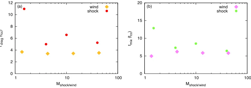
Table2provides normalized values fortdrag,tmix, andtlifefor each
of the simulations presented in this paper. Fig.5also shows the normalized values oftdrag andtmixas a function of the Mach number,
and also in comparison to 2D inviscid shock–cloud simulations with
χ=103. The behaviour of each time-scale is now discussed in turn.
3.4.1 tdrag
First, we note that our wind–cloud simulations all havetdrag/tcc≈
4.2–4.5 (see Table2). These values are typically slightly greater than the values seen from the lower χ wind–cloud simulations in Paper I, which spanned the range 3.3–4.3. Thus, clouds with
χ=103are accelerated by a wind slightly more slowly than those
withχ=10. This dependence is consistent with that also found in shock–cloud simulations (see e.g. Pittard et al.2010), but in both cases the scaling is weaker than theχ1/2 scaling expected from
a simple analytical model (Klein et al.1994; Pittard et al.2010). We also find barely any Mach-number dependence to the values oftdrag/tccin our wind–cloud simulations, whenχ=10 and 103.
0 2 4 6 8 10 12
1 10 100
(a) (b)
t’drag (tcc
)
Mshock/wind
wind shock
0 5 10 15 20
1 10 100
tmix (tcc
)
Mshock/wind
[image:9.595.88.509.57.206.2]wind shock
Figure 5. (a) Cloud drag time,tdrag , (gold diamonds) and (b) mixing time of the core,tmix, (pink diamonds) as a function of the wind Mach number,Mwind
for the wind–cloud simulations. Also shown are the corresponding values from 2D inviscid simulations calculated for a shock–cloud interaction withχ=103
(tdrag, red circles;tmix, green circles). Note that in this figure,tdrag is defined as the time at which the mean cloud velocity,vz, cloud =vps/e, wherevpsis the
post-shock (or wind) speed in the frame of the unshocked cloud. This definition is consistent with Pittard et al. (2010), but differs from Klein et al. (1994) and Pittard & Parkin (2016). Thus,tdrag < tdrag. See Table2for values oftdragcalculated according to the definition given in Section 2.3 of the current paper.
wheretdrag/tccrises sharply at low Mach numbers (e.g. Pittard et al.
2010; Pittard & Parkin2016).
3.4.2 tmix
Table2and Fig.5show thattmix/tccis almost independent of Mach
number for theχ=103wind–cloud simulations presented in this
paper. This behaviour contrasts with that from theχ=10 wind– cloud simulations inPaper I, and the results of Scannapieco & Br¨uggen (2015), where simulations with higher wind Mach num-bers had significantly longer mixing times. Both behaviours contrast with the rapid rise intmix/tccat low Mach numbers in shock–cloud
simulations (Pittard et al.2010; Pittard & Parkin2016). This clearly reveals very interesting diversity between these various interactions and motivates further studies of them. In particular, it is not clear why Scannapieco & Br¨uggen (2015) find longer mixing times with higher wind Mach numbers, when the current work does not, al-though there are a number of obvious avenues to investigate, includ-ing differences between the initial conditions and physics included, the effects of numerical resolution, and differences in the definition of mixing. As a final point, we note that Mach scaling is demon-strated in all of our work (Pittard et al.2010; Pittard & Parkin2016; Goldsmith & Pittard2017), including the present.
Interestingly, Fig.5(b) shows that the values oftmix/tccfrom the
shock–cloud simulations (whichdoshow a Mach number depen-dence) appear to converge towards the Mach number-independent wind–cloud values as Mshock/wind increases. This behaviour,
al-though not quite so clear cut, may also be taking place fortdrag /tcc
too (see Fig.5a). Finally, we note thattdrag /tmix∼0.6 in ourχ=103
wind–cloud simulations (see Fig.5).
3.5 Comparison to existing literature
As noted in Section 1, there is a lack of numerical studies in the literature that investigate the Mach-number dependence of wind– cloud interactions at high density contrast (χ103). Studies which
consider high values ofχ are often limited to a single value of Mwind (e.g. Vieser & Hensler 2007; Cooper et al.2009;
Banda-Barrag´an et al.2016). Thus, it is difficult to draw any conclusions from the current literature as to the Mach-number dependence of tmix in wind–cloud simulations at highχ. In fact, the only other
wind–cloud study, to our knowledge, to investigate a range of Mach numbers at highχis by Scannapieco & Br¨uggen (2015). They find an increasing trend fortmix withMwind, which is in disagreement
with the results that we present here. This disagreement may be related to the different initial set-up (their cloud is initially assumed to be in pressure equilibrium with the surrounding wind, whereas our cloud is underpressured), or to the different physics employed (their simulation is radiative, whereas ours is adiabatic). In addition, there are numerical differences (e.g. 2D versus 3D), and differences in the definition of mixing between their work and ours. Further investigation into the effect of these differences is needed.
In previous shock–cloud studies, Pittard et al. (2010) and Pittard & Parkin (2016) showed that the ratiotdrag /tmixwasχ-dependent.3
To first order, the normalized mixing time-scale is independent ofχ, while the normalized drag time-scale increases weakly with
χ. Thus, clouds with low density contrasts are accelerated more quickly than they mix, while clouds with very high density contrasts tend to mix more efficiently than they are accelerated. At high Mach numbers (Mshock10), Pittard & Parkin (2016) found thattdrag /tmix
increased from 0.14 whenχ =10, to 0.75 when χ = 103. Our
current work now allows us to examine whether such behaviour is displayed in wind–cloud interactions. At high Mach numbers,
Paper Ishowed that forχ=10,tdrag /tmix≈0.1, while here we find
t
drag/tmix≈0.6 forχ = 103. Thus, we find that mixing becomes
relatively more efficient compared to acceleration for wind–cloud interactions as the cloud density contrast increases, in agreement with the behaviour seen in shock–cloud interactions.
4 S U M M A RY A N D C O N C L U S I O N S
This is the second part of a study comparing shock–cloud and wind–cloud interactions and the effect of increasing the wind Mach number on the evolution of the cloud. Our first paper (Goldsmith & Pittard2017) investigated the morphological differences between clouds of density contrast χ = 10 struck by a shock and those embedded in a wind. Significant differences were found, not only between the morphology of the clouds themselves but also in terms of the behaviour of the external medium in each case. It was also
3In these works,t
the first paper to identify Mach scaling in a wind–cloud simulation and additionally found that clouds embedded in high Mach number winds survived for longer and travelled larger distances.
In this second paper, we have continued our investigation of shock–cloud and wind–cloud interactions, but this time have fo-cused on clouds with a density contrast ofχ=103. As inPaper I,
we began our investigation by comparing wind–cloud simulations against a reference shock–cloud simulation with a shock Mach numberM =10 (c3shock). Our standard wind–cloud simulation (c3wind1) used exactly the same cloud embedded in the same flow conditions. On comparing the two simulations, we find only minor morphological differences between the clouds in each simulation whilst the transmitted shock progresses through the cloud. After the transmitted shock has exited the cloud, we find that the cloud in both models begins to develop a low-density turbulent wake. The evolution of the two clouds begins to diverge after this time, and the morphology and properties of the cloud become increasingly different with time. For instance, the development of the wake dif-fers significantly between the two models: the cloud core in model c3shockdoes not fragment but is drawn out along ther=0 axis, whilst that in modelc3wind1 does fragment and eventually disrupts the evolution of the wake.
On increasing the wind Mach number, we find that a super-sonically expanding cavity quickly forms at the rear of the cloud, similar to the higherMwindsimulations inPaper I. This is followed
by a smooth, compressed, thin, but short-lived tail of cloud ma-terial which forms behind the cloud. This narrow tail arises from the focusing of the flow around and behind the cloud. Neither the cavity, nor the subsequent narrow tail, are seen in modelsc3shock andc3wind1, or the comparable models inPaper Iat lowerχ. In all of our new wind–cloud simulations, the cloud eventually fragments and mass-loads the flow.
InPaper I, we demonstrated the presence of Mach scaling in wind–cloud simulations for the first time. Our new results shown here provide further evidence of this effect. For example, the clouds in the higher Mach number simulations are all morphologically very similar (cf. each set of panels in Fig.3), and evolve closely until ‘random’ perturbations caused by the different non-linear devel-opment of instabilities from numerical rounding differences in the simulations eventually cause them to diverge.
We also find that clouds with density contrastsχ >100 can be accelerated up to the velocity of the wind and travel large distances before being disrupted, in contrast to the findings of Scannapieco & Br¨uggen (2015). For instance, in modelc3wind1a, the cloud reaches 90 per cent ofvwindbyt=tmix, at which time it has moved
down-stream≈50rc. However, the flow remains structured and complete
mixing is not achieved.
Our work has helped to reveal a rich variety of behaviours de-pending on the nature of the interaction (shock–cloud or wind– cloud) and the cloud density contrast. In shock–cloud interactions, both the normalized cloud mixing and drag times increase at lower Mach numbers, but are independent of Mach number at higher Mach numbers – i.e. they show Mach scaling (see Klein et al.1994; Pittard et al.2010; Pittard & Parkin2016). The drag time also increases weakly withχ, buttmix/tccdoes not. In contrast, wind–cloud
in-teractions withχ=10 show an almost Mach-number-independent drag time, but a strong rise in tmix/tcc with Mach number until
Mwind∼20, whereupontmix/tccplateaus as Mach-scaling is reached
(Goldsmith & Pittard2017). Our current work reveals another type of behaviour: wind–cloud interactions withχ=103show almost
Mach-number-independent drag and mixing times. Comparison of the current work with Goldsmith & Pittard (2017) also reveals that
the normalized cloud mixing time at high Mach numbers is shorter at higher values ofχin our wind–cloud simulations, which is op-posite to theχ-dependence seen in shock–cloud interactions where tmix/tccis essentially independent ofχ, and at most very weakly
increases with it (Pittard et al.2010; Pittard & Parkin2016). Fi-nally, we find that the Mach number dependent values oftdrag and
tmixfor shock–cloud simulations atχ=103converge towards the
Mach-number-independent time-scales of comparable wind–cloud simulations.
That shock–cloud and wind–cloud interactions display such rich-ness of behaviour demands further investigation. In particular, there is a need to address some of the discrepancies which currently exist between different studies.
AC K N OW L E D G E M E N T S
We would like to thank the referee for their comments which have helped to improve the manuscript. This work was supported by the Science & Technology Facilities Council (Research Grants ST/L000628/1 and ST/M503599/1). We thank S. Falle for the use of theMGhydrodynamics code used to calculate the simulations in this work. The calculations used in this paper were performed on the DiRAC Facility which is jointly funded by STFC, the Large Fa-cilities Capital Fund of BIS, and the University of Leeds. The data associated with this paper are openly available from the University of Leeds data repository (https://doi.org/10.5518/221).
R E F E R E N C E S
Allen D. A., Burton M. G., 1993,Nature, 363, 54
Banda-Barrag´an W. E., Parkin E. R., Crocker R. M., Federrath C., Bicknell G. V., 2016,MNRAS, 455, 1309
Brandt J. C., Snow M., 2000,Icarus, 148, 52
Buffington A., Bisi M. M., Clover J. M., Hick P. P., Jackson B. V., Kuchar T. A., 2008,ApJ, 677, 798
Cecil G., Bland-Hawthorn J., Veilleux S., Filippenko A. V., 2001,ApJ, 555, 338
Cecil G., Bland-Hawthorn J., Veilleux S., 2002,ApJ, 576, 745
Cooper J. L., Bicknell G. V., Sutherland R. S., Bland-Hawthorn J., 2008,
ApJ, 674, 157
Cooper J. L., Bicknell G. V., Sutherland R. S., Bland-Hawthorn J., 2009,
ApJ, 703, 330
Crawford C. S., Hatch N. A., Fabian A. C., Sanders J. S., 2005,MNRAS, 363, 216
Dyson J. E., Pittard J. M., Meaburn J., Falle S. A. E. G., 2006, A&A, 457, 561
Elmegreen B. G., Scalo J., 2004, ARA&A, 42, 211 Falle S. A. E. G., 1991,MNRAS, 250, 581
Fragile P. C., Murray S. D., Anninos P., van Breugel W., 2004,ApJ, 604, 74
Goldsmith K. J. A., Pittard J. M., 2017,MNRAS, 470, 2427 (Paper I) Hennebelle P., Falgarone E., 2012, A&AR, 20, 55
Hora J. L., Latter W. B., Smith H. A., Marengo M., 2006,ApJ, 652, 426 Kaifu N. et al., 2000,PASJ, 52, 1
Klein R. I., McKee C. F., Colella P., 1994,ApJ, 420, 213 Lee J.-K., Burton M. G., 2000,MNRAS, 315, 11
Mac Low M.-M., Klessen R., 2004,Rev. Mod. Phys., 76, 125 Matsuura M. et al., 2007,MNRAS, 382, 1447
Matsuura M., Speck A. K., McHunu B. M., Tanaka I., Wright N. J., Smith M. D., Zijlstra A. A., Viti S., Wesson R., 2009,ApJ, 700, 1067 McClure-Griffiths N. M., Dickey J. M., Gaensler B. M., Green A. J., Green
J. A., Haverkorn M., 2012,ApJS, 199, 12
McClure-Griffiths N. M., Green J. A., Hill A. S., Lockman F. J., Dickey J. M., Gaensler B. M., Green A. J., 2013,ApJ, 770, L4
McKee C. F., Ostriker E. C., 2007, ARA&A, 45, 565 Meaburn J., Boumis P., 2010,MNRAS, 402, 381
Murray S. D., White S. D. M., Blondin J. M., Lin D. N. C., 1993,ApJ, 407, 588
Nakamura F., McKee C. F., Klein R. I., Fisher R. T., 2006,ApJ, 164, 477
Niederhaus J. H. J., 2007, PhD thesis, Univ.Wisconsin, Madison O’Dell C. R., Henney W. J., Ferland G. J., 2005,AJ, 130, 172 Ohyama Y. et al., 2002,PASJ, 54, 891
Padoan P., Federrath C., Chabrier G., Evans N. J., II, Johnstone D., Jørgensen J. K., McKee C. F., Nordlund A., 2014, in Beuther H., Klessen R. S., Dullemond C. P., Henning T., eds., Protostars and Planets VI. Univ. Arizona Press, Tucson, p.77
Pittard J. M., 2011,MNRAS, 411, LL41
Pittard J. M., Parkin E. R., 2016,MNRAS, 457, 4470
Pittard J. M., Falle S. A. E. G., Hartquist T. W., Dyson J. E., 2009,MNRAS, 394, 1351
Pittard J. M., Hartquist T. W., Falle S. A. E. G., 2010, MNRAS, 405, 821 Raga A., Steffen W., Gonz´alez R., 2005, Rev. Mex., 41, 45
Scalo J., Elmegreen B. G., 2004, ARA&A, 42, 275 Scannapieco E., Br¨uggen M., 2015,ApJ, 805, 158
Schiano V. R., Christiansen W. A., Knerr J. M., 1995,ApJ, 439, 237 Schultz A. S. B., Colgan S. W. J., Erickson E. F., Kaufman M. J., Hollenbach
D. J., O’Dell C. R., Young E. T., Chen H., 1999,ApJ, 511, 282 Shafi N., Oosterloo T. A., Morganti R., Colafrancesco S., Booth R., 2015,
MNRAS, 454, 1404
Strickland D. K., Stevens I. R., 2000,MNRAS, 314, 511
Tedds J. A., Brand P. W. J. L., Burton M. G., 1999,MNRAS, 307, 337 Vieser W., Hensler G., 2007, A&A, 472, 141
Yagi M., Koda J., Furusho R., Terai T., Fujiwara H., Watanabe J-I., 2015, AJ, 2015, 149, 97