MoL 2017 28: Understanding Generalization: Learning Quantifiers and Negation with Neural Tensor Networks

with Neural Tensor Networks

MSc Thesis

(Afstudeerscriptie)

written by

Michael Repplinger

under the supervision ofDr. Willem Zuidema, and submitted to the Board of Examiners in partial fulfillment of the requirements for the degree of

MSc in Logic

at theUniversiteit van Amsterdam.

Date of the public defense: Members of the Thesis Committee:

August 31, 2017 Dr. Tejaswini Deoskar

Prof. Dr. Benedikt Löwe (chair) Dr. Jakub Szymanik

The following investigation is focused on the intersection of symbolic and distributional approaches to natural language semantics. Broadly speaking, we analyze symbolic approaches to semantics in order to learn how the performance of distributional models can be improved that are applied to compositional language tasks. Specifically then, we set out to discover empirical justification for the often claimed advantage of employing higher-order tensors in semantic vector space models.

I want to begin by offering my heartfelt gratitude to Jelle, who really was the ideal advisor. You generously offered your time, your insights, and often enough, solid advice that made me wonder if you knew me better than I knew myself.

Thank you, Ulle, Maria, Tanja, for offering guidance, encouragement, and, a chance. Then, a major thank you, Mees, for breaking it down for me with patience and clarity.

And thank you, Marco, Dieuwke, Samira, Sander, Bas and Sara for any number of insightful discussions and uplifting conversations during the writing period.

Thank you Ines, and thank you Umberto. You have supported me for such a long time. I am happy to call you my friends.

For your willingness to listen, and for your ever calm support and guidance: thank you, Andre.

To my mother and sisters, Annemay, Ina, Lilly, Lena: thank you for your patience, and thank you for your unconditional love.

1 Introduction 1

I

Background

2

2 Symbolic and Distributional Semantics 3

2.1 Symbolic Approaches . . . 3

2.1.1 Formal Semantics . . . 4

2.1.2 Natural Logic and Language Inference . . . 7

2.2 Distributional Semantics . . . 10

2.2.1 A Simple Example Space . . . 11

2.2.2 Models and Parameters . . . 11

2.2.3 Neural Word Embeddings . . . 12

2.2.4 Limitations and Relation to Compositionality . . . 15

3 Compositional Distributional Semantics 17 3.1 Two Classes of Compositional Approaches . . . 17

3.2 Types of Composition Functions . . . 18

3.2.1 Additive Composition . . . 18

3.2.2 Multiplicative Composition . . . 19

3.2.3 Combined Models . . . 20

3.2.4 Experiments . . . 21

3.3 Type-Based Compositional Models . . . 22

3.3.1 Background . . . 22

3.3.2 Typed Tensor Model . . . 23

3.3.3 Basic Spaces of Models . . . 25

3.3.4 Limitations of Typed Approaches . . . 26

3.4 Approximative Compositional Models . . . 27

3.4.1 Recurrent and Recursive Neural Networks . . . 27

3.4.2 Memory Mechanisms . . . 29

3.4.3 Tensor-Based Architectures . . . 31

4.2.1 Activation Functions . . . 37

4.2.2 Cost Functions . . . 38

4.3 Recursive Neural Networks . . . 39

4.4 Recursive Neural Tensor Networks . . . 43

4.5 Contrasting Additive and Multiplicative Composition . . . 45

4.6 Learning . . . 47

4.6.1 Learning by Gradient Descent . . . 47

4.6.2 Backpropagation . . . 47

4.6.3 Advanced Optimization . . . 48

4.6.4 Regularization . . . 50

4.7 Conclusions . . . 51

II

Results and Discussion

52

5 Language Inference with Neural Networks 53 5.1 Quantified Inference Task . . . 53

5.2 Model Implementation . . . 54

5.3 Replication of Quantified Task Results . . . 55

5.4 Other Experiments . . . 56

6 Model Representations and Generalization 57 6.1 A Glimpse into the Black Box . . . 57

6.2 Increasing the Task Difficulty . . . 60

6.3 Evaluating Generalization by De Morgan’s Laws . . . 62

6.3.1 Expected Model Predictions . . . 64

6.3.2 Prediction Results . . . 66

6.3.3 Results in Detail . . . 69

6.4 Visualization of Model Representations . . . 71

6.5 Discussion . . . 76

6.5.1 Connecting the Results . . . 76

6.5.2 Limitations and Future Work . . . 77

7 Conclusion 79

III

Appendices

80

A Linear Algebra and Tensor Primer 81 A.0.1 Scalars, Vectors and Vector Spaces . . . 81

A.0.2 Matrices and Linear Maps . . . 82

A.0.3 Tensors and Multilinear Maps . . . 84

B Code Samples 90

Chapter 1

Introduction

Symbolic models of language are fully general; distributional models actually work would be an inappropriate way to introduce a thesis that aims for a nuanced analysis of the two complementary approaches. So we won’t.

Natural language semantics as a field of research has existed for centuries, and our understanding of the rules that describe the language we speak have been examined closely, and with increased formal sophistication. The method by which the under-standing was gained is grounded on symbolic representations, and to many, it appears theonlyway to gain a well-founded understanding of the subject.

More recently however, a new approach has emerged, in its latest incarnation referred to asdistributional semantics. The symbolic definitions and descriptions of the previous approach are replaced here by data-driven methods, and a firm statistical foundation. The focus of this thesis will mostly lie on the latter approach, but with a keen interest in gaining additional insights from the former approach.

The major themes of this thesis relates tocompositionalityof language, and the question how compositionality can be accounted for in models of distributional se-mantics. We will see soon that a related question emerges, regarding the ability or inability of models that solely learn by example, togeneralizefrom the cases they have seen to cases that are new to them. The two themes, of compositionality and generalization, will eventually converge and form a more specific question, regarding the role of higher-order tensors in distributional models.

To address these questions, we experimentally evaluate two related models, one based on a conventional function learned from the data, the other being based on a higher-order tensor. We then describe our qualitative analysis of the experimental results, by visualizing and interpreting the representations the models learned from the data.

Part I

Chapter 2

Symbolic and Distributional

Semantics

This chapter is intended to provide the necessary background to follow the analysis of this thesis. We begin by outlining two approaches to natural language semantics in the symbolic tradition. Next, we introduce some central concepts of linear and multilinear algebra, required to follow the technical details of the models discussed throughout this thesis. The last part of the chapter reviews the literature of distributional semantics. We begin by discussing models of distributional semantics operating at a word level, followed by a review of compositional models, using a broad division of compositional distributional approaches into two classes.

Model Terminology In our analysis we plan to use the following nonstandard

terminology, intended to disambiguate two model classes that will be frequently discussed: Therecursive neural network (Socher, 2014) and the recurrent neural network(Elman, 1990) are both commonly abbreviated as ‘RNN’, in addition to being named similarly. For reasons that will be outlined in Chapter 4, we usually prefer to describe the model of Socher (2014) as atree-structuredrecurrent neural network, using the abbreviationtRNN. Analogously, we abbreviate the relatedrecursive neural tensor networkastRNTNin our thesis.

2.1

Symbolic Approaches

2.1.1

Formal Semantics

Tradition demands that discussions of formal semantics begin by citing the well-known principle of compositionality. Despite its abstract nature, the principle can be interpreted as the foundation of modern theories of formal semantics – providing a motivation to discuss it besides tradition.

Principle of Compositionality Theprinciple of compositionality, generally associ-ated with the works of Gottlob Frege (Frege, 1892), is commonly phrased along the lines of: “The meaning of a complex expression is determined by the meanings of its constituents and the rules used to combine them.” In its abstract form, the principle leaves many aspects of semantic analysis unspecified. Nonetheless, two constraints can be identified: Studying the meaning of language requires analyzing the meaning of individual components, as well as the rules by which we construct larger expressions from smaller ones.

Closely related to compositionality is the notion ofrecursion. Recursively defined processes are widely believed to underly the capacity of speakers of a language to build and understand arbitrary expressions of the language. By recursivesyntactic processing, speakers can, in principle, build an infinite set of complex expressions from a finite set of simple “building blocks”. By a parallel recursivesemanticprocess, speakers are then able to express and understand a potential infinitude of distinct meanings.

From Principles to Theories The following lucid description of compositionality

is offered by Barbara Partee:

The compositionality requirement . . . is almost uncontroversial when stated informally. But formalizing it requires an explicit theory of syntax, an explicit theory of semantics, and an explicit theory of the mapping from one to the other.1

Based on the general description of a grammar in Montague (1970b), Partee (2014) adds that these “explicit theories” can be understood as syntactic and semantic alge-bras, together with a homomorphism instantiating the mapping. While still allowing considerable theoretical variation, the principle gained concreteness under this view: The objective of the syntactic algebra is to construct complex expressions (phrases and sentences) from the basic ones (words) by recursive operations, ideally deriving a set of expressions that is identical to the expressions encountered in natural language.2

While natural language expressions can be ambiguous, once a (logical) transla-tion has been determined – possibly several distinct translatransla-tions for an ambiguous expression – by the homomorphism requirement we ensure that any element of the syntactic algebra is mapped to a unique element of the semantic algebra. The latter

1 _{Partee (2001). Parenthetical remarks omitted.}

provides expressions with meaning, often through model-theoretic interpretation, while the homomorphism requirement ensure that each expression is assigned exactly onesuch interpretation, thus formally specifying the “meaning functionality” demand expressed abstractly by the original principle.3

In this form, the principle admits a general framework offormal semantics, se-mantic theories using the language of mathematics, following the spirit of Frege’s principle. Next, we will sketch the basic principles of Montague Semantics – arguably the most influential semantic theory, and the proposal which established the formal understanding ofcompositionalityin the sense outlined above.

Montague Semantics Montague Semantics or Montague Grammar, developed mostly in a series of seminal papers Montague (1970a,b, 1973), is widely considered to be the first successful attempt to fully formalize the semantics of natural language, or at least some fragment of it.

While the earlier Montague (1970a) showed that the direct interpretation of ex-pressions, without an intermediate logical language, is possible in principle, the system developed in Montague (1970b) and Montague (1973) proved to be more popular, proceeding by translation of natural language expressions into an intermediate logical language, followed by interpretation by model-theoretical semantics. It is the latter approach we will outline in here.

In broad terms, Montague’s innovative proposal consists of the compositional translation from natural language to a logical language, such that (syntactic) deriva-tion proceeds in parallel to assignment of semantic representaderiva-tions. This parallel definition ensures that each derivation of a sentence is assigned a unique and appro-priate meaning by the theory. The synchronous processing of syntax and semantics is made available by Montague’s highly expressiveintensional logic, a higher-order typed (intensional) logic, enriched by lambda abstraction allowing the construction of appropriate functions at each derivation step.

Our sketch of Montague’s system omits several features that were revolutionary at the time, but are now standard techniques of the field, such as generalized quantifiers, or ‘extensionalizing’ intensional expressions via possible worlds. We refer interested readers to Gamut (1991) or Heim and Kratzer (1998) for thorough introductions to semantic systems in the spirit of Montague’s proposal.

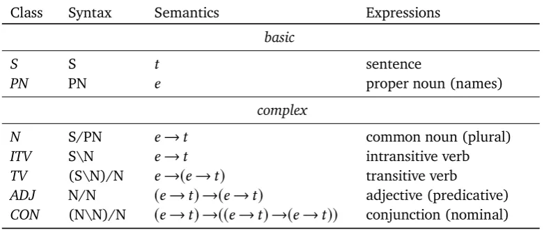
Toy Grammar We exemplify the meaning derivation process, outlined in general

terms above, by an example sentence and a toy syntax, given in the form of a (sim-plified) categorial grammar. Table 2.1 describes the syntactic categories and their corresponding semantic types: Names are of syntactic category PN (proper nouns), and semantic type

e

, a basic type of entities, interpreted as elements of the domain of discourse. Transitive verbs are of category TV, interpreted as a function from entities to a function from entities to truth values, of type

(

e

→(

e

→

t

))

. Composition of a

3 _{Note that by choice of a homomorphism between syntax and semantics, every syntactic expression is}

Class Syntax Semantics Expressions basic

S S

t

sentence

PN PN

e

proper noun (names)

complex

N S/PN

e

→

t

common noun (plural)

ITV S\N

e

→

t

intransitive verb

TV (S\N)/N

e

→(

e

→

t

)

transitive verb

ADJ N/N

(

e

→

t

) →(

e

→

t

)

adjective (predicative)

[image:12.595.103.494.125.290.2]

CON (N\N)/N

(

e

→

t

) →((

e

→

t

) →(

e

→

t

))

conjunction (nominal) Table 2.1: Correspondence between syntax and semantics

transitive verb with its object results in category VP (a verb phrase), interpreted as a function from individuals to truth values,

(

e

→

t

)

. Finally, the full sentence is of category S, of basic type

t

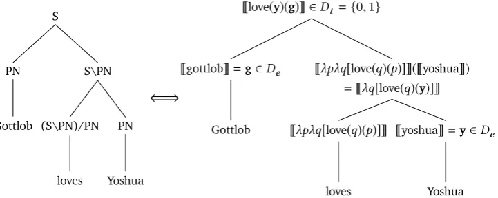
of truth values, and interpreted as ‘true’ or ‘false’.

The left side of Fig. 2.1 is a parse tree of the example sentence “Gottlob loves Yoshua”, under the syntactic rules expressed by the complex syntactic types in Table 2.1. Analogously, the right tree shows the result of assigning each node on the left a meaning. The meaning of the names are logical constants, interpreted as domain elements, while the meaning of the verb is a lambda expression over two individual evaluating whether they stand in the relation denoted by the relational constant. These meaning assignments are lexical, while the assignments of the remaining nodes result from rules that are the semantic analog to the syntactic phrasal rules. They correspond here to function-argument application, first for the object of the transitive verb, then the subject. The phrasal nodes on the right also contain the expressions resulting from beta reduction, replacing free occurrences of a parameter variable with the argument value. The topmost node, representing the meaning of the entire sentence, yields ‘true’ if the denoted individuals stand in the denoted relation, and ‘false’ otherwise.

Note that the bidirectional arrow between trees should not be read as saying that every sentence has a unique logical translation, and therefore, a unique meaning. It is intended to show that sentences, given a particularsyntactic derivationare assigned a unique interpretation.

Criticism and Alternatives The field of modern formal semantics increased the

for-mal understanding of language meaning substantially over the past decades. Nonethe-less, criticism of the approach can be raised, of which we give two examples.

S

S\PN

PN

Yoshua (S\PN)/PN

loves PN

Gottlob

⇐⇒

nlove(y)(g)_o∈D_t ={0,1}

nλpλq[_love(q)(p)]_o(_nyoshuao)

=nλq[_love(q)(y)]_o

nyoshuao=y∈D_e

Yoshua nλpλq[_love(q)(p)]_o

loves ngottlobo=g∈D_e

[image:13.595.112.473.126.270.2]

Gottlob

Figure 2.1: Translation to logical language

learning models, raising the question whether similar approaches could be applied to compositional meaning analysis.

Another point concerns the limited integration of individual semantic theories. Mon-tague’s original proposal was a “method of fragments” – identifying a well-delineated syntactic fragment of the language, then formally describing this fragment. Modern semantic theories mostly no longer take this approach, opting instead for the descrip-tions of particularsemantic phenomenathat are not confined to a syntacticfragment. Consequently, no part of the language can be set aside and semantically described incompletion, which is a requirement however forcomputationalmodels of symbolic semantics (Partee, 2001).

The theoretical question whether there are viable alternatives to symbolically grounded semantics is part of a long-running debate, for example, in the discussion of thebinding problem. We will not attempt to directly answer this complex question here, but will indirectly address it throughout our analysis.

2.1.2

Natural Logic and Language Inference

Natural logicgenerally describes logical systems encoding reasoning patterns encoun-tered in natural language, in contrast to classically defined logic, cenencoun-tered around the notion of formal validity of inference, orlogical reasoning. The termnatural logic, and the framing of the problem in a modern logical context, is due to Lakoff (1970). One application of natural logics is the modeling ofnatural language inference(NLI), automated systems performing reasoning tasks over natural language expressions.

Symbol Name Example Interpretation

x

≡

y

equivalence (couch, sofa) X =Y

x

@

y

forward entailment (excl.) (crow, bird) X ⊂Y

x

_A

y

reverse entailment (excl.) (bird, crow) X ⊃Y

x

∧

_y

_{negation (able, unable) X∩Y =∅ ∧X∪Y =U}

x

|

y

_{alternation (cat, dog)} X∩Y =∅ ∧X∪Y _,U

x

`

y

cover (animal, non-dog) X∩Y _,∅ ∧X∪Y =U

[image:14.595.102.493.124.235.2]

x

#

y

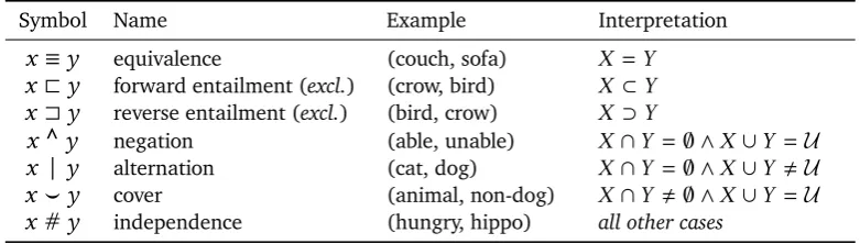
independence (hungry, hippo) all other cases

Table 2.2: The seven basic relations of MacCartney’s logic4

monotonein both arguments. Consider next that “Every European sings” entails “Every German sings”, but does not entail “Every European sings loudly”. However, “Every European sings loudly” entails “Every European sings” – we say ‘every’ is downward monotone in its first argument andupward monotonein its second argument.

MacCartney Logic and NatLog The natural logic developed in MacCartney (2009)

is described by the author as an extension of the monotonicity calculus by Valencia (1991) and van Benthem (1991). The logical model has been implemented compu-tationally as theNatLogsystem, outlined for example in MacCartney and Manning (2009). The inference mechanism of MacCartney’s natural logic operates directly on natural language expressions, without intermediate translation to a logical language – similar to the original Montague framework mentioned in Section 2.1.1.

Traditionally, inference of language is modeled in terms of two relations, entail-ment, and contradiction, sometimes adding a third, independence. MacCartney’s system defines seven relations, in order to adequately cover the entire spectrum of natural language inferences. The seven basic relations, with examples and their set-theoretic definitions, are listed in Table 2.2. Some relations are familiar (equivalence, entailment, independence). Note that entailment is split over two relations, with two corresponding symbols: forward entailment and reverse entailment. Next, ‘negation’ relates mutually exclusive concepts whose union covers the entire domain; ‘alternation’ relates mutually exclusive items whose union does not cover the domain; ‘cover’ relates overlapping concepts whose union covers the domain.

The basic relations are related to monotonicity by the projective properties of expressions. For example, “fail to

x

” is downward monotone: “fail to sing” entails “fail

to sing loudly”. Its projective property with respect to

@

, the entailment relation inside the logic, is characterized by a direction reversal: “Sing loudly”

@

‘sing’, but: “fail to sing loudly”

A

“fail to sing”. In total, these projective properties of expressions over the basic relations characterize howcontextinfluences thecompositionof inference – in a sense which will be made more precise next.

Compositional Entailment The system described so far only derives direct lexical

instances of entailment, i.e. from one word to another. Extension to the (propositional) sentence level is intuitively straightforward, by interpretation of propositions as sets of possible worlds. For instance, “all dogs bark” and “not all dogs bark” are related by the basic relation ‘negation’; their sets of worlds are disjoint, and the union of their worlds contains all possible worlds (by the law of excluded middle).

The next extension consists of adding compositionality to the system, to allow inferences beyond a single step. To this end, the logic is equipped with a simple proof calculus. Compositional derivations proceed via a sequence ofedit operations, i.e. an algorithmic replacement process, which encodes both lexical knowledge and the monotonicity contributions by the context, e.g. of quantified subexpressions. The atomic edit operations are:

substitutions are one-for-one lexical replacements yielding the relation that holds between the replaced items, e.g. ‘sofa’

7→

‘couch’ yields:

≡

deletions replace a complex expression by a simpler one, usually on items under entailment, e.g. “red car”

7→

‘car’ yields:

_@

insertionsare defined symmetrically to deletions, so for items under reverse entailment, e.g. ‘car’

7→

“red car” yields:

_A

Given a premise and a hypothesis, complex inferences are performed as a series of these edits, in which the edit sequence transforms the premise into the hypothesis. The (predicted)relationholding between the premise and hypothesis is then determined as follows: Each edit of the sequence is associated with a relation (e.g. the relation that held between two words that were substituted). These chained edits are then joined to form (ideally) a single predicted relation. The main complexity of this process is to determine how relations are joined, given their context. To this end, the process is defined as a function of the monotonicity or projective properties described above, ensuring that the outcome of joining takes into account the monotonicity properties of the context in which the edit that generated the relation took place.

Limitations of the Logic MacCartney and Manning (2009) evaluate an

implemen-tation of the logic on several semantic tasks, and performance on the tasks suggests that the edit-based proof calculus is sufficient for the primary aim of the system of modeling natural language inference. Seen as a formal logic however, the authors note that the deductive power of the system is strictly lower than that of classical first-order logic. For one, the system does not allow combination of multiple premises, i.e. the classical syllogisms based on two premises and one conclusion are not directly representable in the system.

This duality, commonly known as thede Morgan’s laws for quantifiersin classical first-order logic, expresses:

∀

xP

(

x

) ≡ ¬[

_∃

¬

P

(

x

)]

(2.1)

∃

xP

(

x

) ≡ ¬[

_∀

¬

P

(

x

)]

(2.2)

This deductive limitation in terms of quantifier equivalences will gain practical rele-vance in Chapter 6, where its effect was instrumental for one of the results.

2.2

Distributional Semantics

We turn now to the models of distributional semantics, explaining the rationale behind the models and discuss their advantages and limitations.

The following sections presuppose some basic knowledge of linear algebra and tensor calculus. For readers who want to refresh their memory, a brief linear algebra primer is provided in Appendix A. In this primer we also introduce the basic concepts behind higher-order tensors, and briefly touch on a few related points, such as tensor factorization and the difference between the definition of tensors in the machine learning literature and in pure mathematics.

Distributional Hypothesis Models ofdistributional semantics, or semantic vector space models, are a class of semantical models based on statistical and machine learning techniques, usually understood as realizations of thedistributional hypothesis. Following Firth (1957), the hypothesis is often expressed as: “A word is characterized by the company it keeps”. The related idea, of language meaning being defined by language usage, can be traced back further to a central concept of Wittgenstein (1953). Paraphrasing, the hypothesis states thatsemantic similaritycan be expressed bydistributional similarity, suggesting that statistical analysis of language is an effective way of determining word meaning.5

Spatial Representation While the above suggests a method to gather semantic

information, we also require a formal system torepresentthe information. All models discussed here arevector spacemodels, in which words correspond to elements of that space, i.e. each word is represented by a vector. Given this representation, semantic similarity between words can be defined in terms of distance between their vector representations. More generally, a vector space representation enables spatial or geometric interpretation of semantic meaning, providing the semantic theory with the complete formal machinery of (finite) vector spaces. In particular, a natural extension ofcompositionalsemantics is provided, leading to the models discussed in Chapter 3.

5 _{We will sometimes refer to the methods of this section as belonging tocontextualdistributional}

animal large small USB

mouse 8 2 4 3

elephant 9 5 1 0

car 1 4 3 0

Table 2.3: Idealized context-counts for mouse, elephant and car

2.2.1

A Simple Example Space

Table 2.3 is an idealized illustration of co-occurrence counts and a corresponding semantic space for three nouns, ‘mouse’, ‘elephant’ and ‘car’. Values in this table indicate how often a target word, i.e. the word we aim to represent as a vector, appeared near certain other words in a corpus. For example, ‘mouse’ and ‘animal’ co-occurred eight times, while ‘car’ and ‘animal’ did so only once. Based on these hypothetical counts, our semantic space would be four-dimensional, with vectors consisting of raw co-occurrence counts. In reality, dimensionality is usually in the order of hundreds, and raw counts are transformed into (weighted) frequency values.

Using cosine similarity defined in Appendix A on pairs of these word vectors, we can calculate their semantic similarity: 0.86 (mouse, elephant), 0.57 (mouse, car), 0.61 (elephant, car). This would then represent, as intended, that ‘mouse’ and ‘elephant’ are more similar to each other than either of the two is to ‘car’ (animals vs. non-animal), and that ‘car’ is (slightly) more similar to ‘elephant’ than to ‘mouse’ (being somewhat more similar in size). Note also the co-occurrence of ‘mouse’ with a seemingly unrelated word, ‘USB’, intended to illustrate the problem ofpolysemy. In most models, the vector representation of ‘mouse’ would be a ‘mix’ of contexts where ‘mouse’ refers to a rodent and contexts where the word refers to a computer component.

2.2.2

Models and Parameters

We now present some important choices and parameters in the definition of distribu-tional semantic models, exemplifying these choices by relevant models implementing them in certain ways.

Context Several parameters and modeling choice are left to be defined in specifying

topic models, use an entire document as context, deriving a low number of (latent) topics which are defined by distributions over words.

Similarity Another modeling choice, although not strictly part of the “meaning

extraction” architecture itself, is thesimilarityordistance metric. Choosing a par-ticular metric, like cosine similarity, implicitly encodes certain assumptions about what constitutes semantic similarity, in addition to being motivated by statistical considerations.

Weighting While all models, in some form, derive semantic information from the

analysis of lexical co-occurrence, i.e. are based oncontext counting, most do not use unprocessed counts to populate the vector components, but instead transform them by weighting schemes. Intuitively, these processing steps can be seen as adjusting counts for word frequency, giving more weight to words that are rare but informative. For example, a word that occurs frequently and across several unrelated meaning contexts, is semantically less informative than a word that occurs infrequently, and only within a small number of related contexts. Weighting is aimed at discounting the contribution of the former words, while giving more weight to the latter. A popular method used for this purpose ispointwise mutual information(PMI).

Dimensionality Several approaches performdimensionality reductionon the derived representations. A common processing pipeline, described for example in Baroni et al. (2014b), roughly proceeds as follows: construct co-occurrence matrices from corpus analysis, re-weight counts by PMI, compress matrices by non-negative matrix factorization (NMF) or singular value decomposition (SVD). The dimensionality reduction step is motivated by two main concerns: computational efficiency, and possibly greatergeneralizationcapacity of the model Levy and Goldberg (2014). The latter effect can result from merging (similar) contexts, i.e. associating a word with contexts of similar words even though it might have never appeared directly in these contexts itself, thus allowing the model to uncover additional similarities.

Objective A fundamental choice not explicitly mentioned so far is theobjectiveof the algorithm analyzing the data. The classical method, described above, is aimed atcounts of context items of a given word. A recent class of models, neural word embeddings, instead aims topredict, either (the most likely) word given a context, or the (most likely) context for a given word. We will discuss the difference between objectives in the next section.

2.2.3

Neural Word Embeddings

Sparse vs. Dense Word-level models of distributional semantics can be

distin-guished by the type of their vectorial representation. First,sparserepresentations – high-dimensional spaces in which dimensions directly correspond to contexts, conse-quently leading to vector representations that are numericallysparseacross compo-nents, since a word does not appear in every context. The classical counting approaches, possibly including count re-weighting, but excluding dimensionality reduction, would fall into this category. Second,denserepresentation – (usually) lower-dimensional spaces, in which dimensions are the result of compressing (classically) derived counts by dimensionality reduction, or are constructed densely immediately, i.e. as embed-dings.

History The latter approach is taken by models referred to as neural language

models ofword embeddings. These models are usually traced back to early suggestions by Hinton (1986), and Bengio et al. (2003), who applied a (regular) neural architecture to the task of deriving word meanings. Embeddings gained an immense boost in popularity after the proposals by Mikolov et al. (2013b) and Mikolov et al. (2013a), implemented as

word2vec

. These methods can be understood as feedforward neural

networks without hidden layers and nonlinear activation functions, which the authors identified as computational bottlenecks of the previous models.

word2vec The embeddings created by word2vec consist of two distinct, but closely

related algorithms. The first model,Continuous Bag-of-Words(CBOW), learns topredict a word, given a context of surrounding words. A “projection layer” turns discretely encoded (sparse) word representations into continuous (dense) representations, which are then fed into a matrix – shared for all context words regardless of their position, hence the name “bag-of-words” – for an output prediction of the most likely middle word for a given context. The second models is trained to predict in the opposite direction; given a word, the goal is to maximize the log probability of its surrounding context, i.e. the model learns topredict the context, given an individual word. Note that the context words do not need to appear as a consecutive sequence in the corpus, i.e. the total number of context words is fixed by a parameter, but individual words can be skipped– referred to by the algorithm’s name. The above sketch of the algorithms only describes the “bare-bones” method, omitting for examplenegative sampling, which can roughly be understood as an approximation of the softmax function needed for the conditional probability training objective.

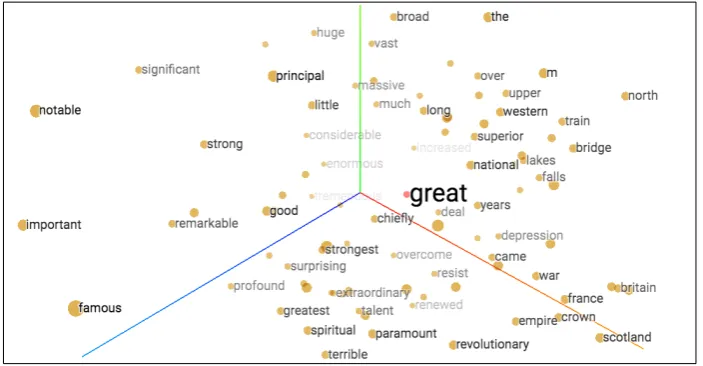
Embedding Advantages In contrast to previous proposals of neural embeddings,

[image:20.595.123.475.123.306.2]

Figure 2.2: word2vec embedding ofgreatand neighboring embeddings6

embeddings sparked additional interest due to linguistic regularities seen in these models, suggesting an interpretation in terms of semantic features. We will discuss these regularities in the following paragraph.

It is currently an open question whether the representations of neural word models are substantially different from those of the classical word models. A study by Baroni et al. (2014b) concludes that (prediction-based) neural embeddings generally outper-form the classical (count-based) methods. This result has been challenged by Levy and Goldberg (2014), which formally establish a close correspondence between the neural models and models factorizing PMI matrices, i.e. claiming that prediction models are equivalent to counting models. Further empirical evidence for this claim was provided in Levy et al. (2015), showing that counting models can achieve performance similar to embeddings by improved hyperparameter choices. In response to these rebuttals, Arora et al. (2015) argue formally and empirically that embedding models, like those of word2vec, are not reducible to matrix factorization if one makes realistic assumptions regarding model dimensionality. Further, these modelsimposethe linear structure on the data by theirlow-dimensional,nonlineararchitecture, suggesting that embedding models are more powerful than classical higher-dimensional approaches.7 Linguistic Regularities Neural embeddings gained widespread attention for their

representation of relatively complex syntactic and semantic relational information, at odds with linguistic expectations of a syntactically shallow, unsupervised model. Further, these linguistic relations can be extracted from the model by simple linear

6 _{1st/2nd/3rd principal component of 200D word2vec embeddings. Plot generated with TensorFlow}

Embedding Projector (Smilkov et al., 2016).

7 _{While word2vec models contain no hidden layers with nonlinearities, they are nonlinear models due}

operations over representations, suggesting that embeddings contain non-trivial linear structure.

Several well-known examples of such relations were presented in Mikolov et al. (2013c). Here, the authors observe that a relation-specific, constantvector offsetexists between the vector representations of word pairs standing in the given relation. Based on this offset, the embedding space can be queried for an answer toanalogy questions of the form: “word 1 is to word 2 as word 3 is to word 4”, where words 1, 2, 3 are given, and word 4 needs to be found in order to answer the question. Expressed in terms of vector space operations, using cosine similarity to measure semantic similarity, the analogy query is given by:

argmaxv₄

(

cos

(

v4

,

v3

−

v1

+

v2

))

(2.3) The following are some well-known results derived by this query:

v_king

−

v_man

+

v_woman

≈

v_queen

v_Paris

−

v_France

+

v_Italy

≈

v_Rome

v_apple

−

v_apples

≈

v_car

−

v_cars

The first result can be understood as the vector form of the analogy “manis towoman as kingis to queen”, expressed in terms of basic linear algebraic operations. This example has been interpreted as evidence that embeddings contain structure encoding a gender relation or feature. Similarly, the next two examples suggest the model learned to relate countries and their capitals, as well as asyntacticrelation between singular and plural word forms.

2.2.4

Limitations and Relation to Compositionality

While the relevance of the previous results should not be easily dismissed, it seems doubtful whether purely context-based models can model meaning in its full generality, over arbitrary types of expressions.

Limits of Context Learning An apparent limitation relates to the meaning of

sentences, widely believed to require accounting forcompositionality. A purely distri-butional, non-compositional approach to sentence meaning is likely to face serious obstacles due to anunanalyzedtreatment of sentences or phrases. Sparsity of datais one such obstacle. Individual words occur abundantly across different contexts, but the frequency of combinations of words declines with the length of the sequence. While short phrases still occur frequently enough to enable some form of meaning deriva-tion by contextual analysis alone, full sentences occur too rarely for a context-based approach aimed at general sentence meaning.

assumption is countered empirically. Researching distributional patterns ofcontrasting word pairs, Mohammad et al. (2013) show that highly contrasting items (including aspectual negation) occur in very similar contexts – indicating that logical negation cannot be learned by context analysis alone.8

Generalization Capacity Finally, another concern relates to the capacity of speakers

ofgeneralizationover meanings of expressions. Human speakers frequently encounter sentences they have never heard before, yet, they easily derive their meaning by knowing the meaning of the individual components (words) and how to combine them systematically (the rules of composition). It seems clear to us that the purely contex-tual distributional models are capable ofsomegeneralization, considering empirical evidence such as the structure exposed by the analogy results, or formal results like the linearizingeffect of embeddings shown by Arora et al. (2015). It seems similarly evi-dent to us however that distributional approaches without any mechanism accounting for compositionality are unlikely to be capable offullgeneralization. Otherwise, the meaning of complex expressions of arbitrary depth and structural complexity would be fully defined by their usage distributions. This notion however is both at odds with linguistic theory and unwarranted from a statistical perspective, considering the aforementioned problem of data sparsity with respect to sentence length.

Combination of Approaches The limitations outlined here seem to motivate

com-positional extensions of the distributional approaches. At the same time, the success in some aspects of meaning derivation of these models is undeniable. Distributional approaches constitute a major step forward in the derivation of lexical meaning – an area of research comparably underappreciated by symbolic theories of meaning. It also seems to be widely accepted that several breakthrough results achieved by deep learning models in recent years were made possible by including (pre-trained) word representations. The goal therefore seems to be tocombinedistributional models with compositional processing. Under this view, the question: “What are the limitations of distributional models in deriving sentence meaning?”, could perhaps be rephrased as: “What are the limitations of current distributional models when used asinputfor furthercompositional processing?”

8 _{Kruszewski et al. (2017) confirm that logical negation eludes context analysis, but show that}

Chapter 3

Compositional Distributional

Semantics

In the previous chapter, we saw an outline of the symbolic approach to compositionality, as well as the areas of success and limitations of context-based models of Section 2.2. Next, we will turn to the literature oncompositional distributional semantics. In broad terms, the models of this approach extend the contextual methods of distributional semantics by elements that allow for the derivation of phrasal and sentential meaning.

3.1

Two Classes of Compositional Approaches

Before continuing our review, we first propose a (nonexhaustive) classification of recent compositional approaches to distributional semantics. The classification, far from covering the entire field, is merely intended as a lens through which we suggest viewing the literature. It will allow us to focus the discussion on two prominent research directions, and maximize the contrast of their comparison. We suggest then a division along the following classes:

type-based(ortyped) approaches, with models of this class employing higher-order tensors under an explicit syntax-semantics correspondence

approximative approaches, generally relying on machine learning techniques to

indirectly represent and approximate the effects of composition

Examples of the type-based approach are the framework of Baroni et al. (2014a), or the approach outlined in Coecke et al. (2010). We refer to this class of models astype-based approaches, because they can be understood as a translation of symbolic semantics to a vector space framework, by defining a correspondence between syntactic categories, semantic types and tensor order.

can be seen as explicitly stating the compositional rules, models of the second approach are aimed instead atlearningthe parameters of composition, generally through some form of approximation.1

Before reviewing the literature under the view of this classification, we will discuss two studies that do not fall under it, but which had a major impact on the entire field of compositional distributional semantics.

3.2

Types of Composition Functions

This section discusses two landmark articles, Mitchell and Lapata (2008) and Mitchell and Lapata (2010), which frequently serve as a starting point in the literature of compositional methods in distributional semantics. These early investigations of compositionality should be seen in the context of another highly influential study, Turney and Pantel (2010), published at around the same time. Where the studies of Mitchell and Lapata provide an overview of composition methods, the study of Turney and Pantel (2010) covers the entire field of distributional semantics, classifying and discussing models, their methods and underlying assumptions. Up until the point when the embedding models of Section 2.2.3 rose to prominence, the study of Turney and Pantel provided a near-complete overview of the methods of (count-based) distributional semantics.

Shared Model Features Input to all models consists of word vectors constructed by

contextual word models, as described in Section 2.2. In the evaluation of Mitchell and Lapata (2010)compositionis implemented as the application of a function mapping two vectors (the composition input) to another vector (the composition output), in a single composition step. Recursive extensions of the following definitions seem to be straightforward, but were not investigated, since the experimental setup only requires a fixed number of composition steps.

3.2.1

Additive Composition

The general definition of theadditiveclass of models is:

z

=

V x

+

W y

where

V

_,

W

_{are matrices, and composition is given by matrix multiplication.}

The simplest instance of this class is given by vector addition:

z

=

x

+

y

which we obtain from the general definition by letting

V

,

W

be identity matrices. The authors note several limitations of this approach, among them, insensitivity to word order, due to commutativity of vector addition. Consider for example that

recursive application of vector addition would derive identical meanings for the phrases “man bites dog” and “dog bites man”. The model’s only advantage seems to be its conceptual simplicity and absence of parameters requiring optimization. Yet, despite its simplicity, the method performs comparably well on the task.

Adding scalar weights for each vector results in theweighted additivemodel:

z

=

α x

+

β y

Here, left and right input vectors are scaled (uniformly, for each vector) by parameters

α

,

β

which are optimized on a development set. For

α

,

β

, this introduces some limited form of syntactic awareness, since left and right input are scaled differently during composition.

Blending Problem While adding weights partially counteract the problem due to

commutativity described above, the authors observe another fundamental problem, referred to asblendingof meaning: Summing, or, equivalently, under cosine evaluation, averagingcomponents of the input vectors results in a blend of features in the output. The problem is illustrated by the example phrase “brown cow”. Its intended meaning refers to something that is both brown and a cow, i.e. the composed meaning is more specificthan that of its constituents, ‘brown’ and ‘cow’, individually. Additive composition however appears to have the opposite effect: the output vector is a sum of the constituents’ components, forming a blend of their properties, thus deriving a less specific, “in-between” meaning, according to the authors.

3.2.2

Multiplicative Composition

Multiplication of components is suggested as a solution to theblendingproblem above, leading to a general form ofmultiplicativemodels:2

z

=

V

xy

where

V

_{is a 3rd-order tensor mapping the two constituent vectors}

x

_,

y

_{to output} vector

z

_{. Composition is consequently a bilinear function of the constituents.}

The first example of this class is composition byelement-wise product:

z

=

x

y

Here, the

i

-th component of output

z

only depends on the

i

-th components of input

x

,

z

, in analogy to vector addition above. However, the interaction between components is now multiplicative instead of additive, as before.

Consider then why multiplication of components can be seen as a solution to the blending problem: Additive interaction does not relate input components directly, i.e. the components of input vectors are added (possibly scaled by a constant factor) to the output vector, independently of any other components. Instead, if composition is

defined in terms of component multiplication, values interact directly by their products. For example, consider some component with a high numerical value interacting (by multiplication) with another component with a value (near) zero . Despite its high value, the meaning contribution of the former is limited by its interaction with the latter, effectively barring it from significantly influencing the meaning of the composite expression. If additive composition can be seen as featureblending, then this type of interaction can be thought of as featurefiltering.3

Tensor-Based Composition While multiplicative interaction might solve the

prob-lem of meaning blending, the simple multiplicative model above is still insensitive to word order. To rectify this problem, thetensor productmodel is introduced:

z

=

x

⊗

y

While the element-wise product before only allowed interactions between components with identical indices, the full tensor product of two

d

-dimensional vectors

x

and

y

, seen as a

d

×

d

matrix, contains the products of all possible component combinations over the two vectors. This model can be related to earlier proposals, such as Smolensky (1990), where the tensor product acts as a universal operator for variable binding.

Note that the tensor product is not commutative, so composition is no longer insensitive to word order. The downside is an exponential increase in dimensionality (from constituents of

R

d to output of

R

d2), and a uniform meaning contribution of all component combinations, due to a lack of parameters.

Two more complex multiplicative models are introduced, both defined on the basis of higher-order tensors. The first,circular convolution, performs modular addition along the diagonals of the tensor product in matrix form, compressing the tensor product to a vector of the same size as the input. The second,dilation, is defined in terms of a 4th-order tensor, and can be seen as a basis-independent variant of the element-wise product model, where the output consists of input vector

y

_{scaled in the}

direction of input vector

x

by a constant factor.

3.2.3

Combined Models

Combined models, models using both additive and multiplicative composition, are briefly mentioned in Mitchell and Lapata (2008), defined as:

z

=

α x

+

β y

+

γ x

y

We can see that this class is simply the summation of the previously defined weighted additive and element-wise product models.

The combined class is of additional interest because it shares some characteristics with the RNTN architecture and its tensor-based composition function. While the combined model above and the RNTN tensor differ in complexity, they both combine

additive and multiplicative elements for composition, and can be seen as belonging to the same class of models therefore.4

3.2.4

Experiments

Mitchell and Lapata (2008) and Mitchell and Lapata (2010) evaluate the models by comparing their predictions to human judgment on a (phrasal or sentential) similarity task. For the model prediction, two phrases are processed compositionally, each phrase yielding a single vector. These vectors are then compared by cosine similarity, yielding a prediction of theirsemantic similarity. The same phrase pairs are judged by humans, and model performance is defined as correlation between the model’s prediction and the human rating.

In the first set of experiments, multiplicative models generally outperform ad-ditive models across word class categories. In particular, the element-wise product model significantly outperforms (almost) all other models. The only exception is the verb+object category, where the dilation model performs approximately equal. The

simplest additive model (vector addition) performs badly across categories, but the weighted additive model comes close to the performance of the multiplicative models, taking second or third places across categories, in an evaluation consisting of seven compositional and two non-compositional models.

In a second set of experiments using a LDA topic model, results are less conclusive, with no individual model outperforming all others across classes. Further, the gap between additive and multiplicative models all but disappears. The weighted additive model continues to perform well in this setting, while performance of the element-wise product suffers.

Significance of Results The results of Mitchell and Lapata (2008, 2010) have

occasionally been used as evidence against (syntactically) complex composition, due to the relatively strong performance of the simple element-wise models. Such conclusions seem doubtful however, considering that the task of Mitchell and Lapata (2010) used composition input from syntactically shallow bag of word models, and comparably inexpressive versions of the complex composition operations. While the input vectors are possible structured meaningfully, they likely require additional ‘restructuring’ during composition. The parameter-free tensor product model, while being non-commutative, has no means of imposing structure on the input, or reshaping the structure to fit the task. The parametrized models possess some means to do so: The weighted additive models can balance the left against the right argument, while dilation adjusts to which degree one input vector scales the meaning of the other. Yet neither of them fully reshapes input on a more fine-grained level, in contrast, for example, to a fully parametrized linear or bilinear map. In conclusion, it seems that the

4 _{Combined modelsare also called “mixture models” in the literature. Note however that other authors}

complex composition method were at a disadvantage compared to the simple methods, given that theireffectivesyntactic sensitivity was limited by a lack of parameters.

It seems that if an investigation similar to Mitchell and Lapata (2010) would be undertaken today, more powerful versions of the original composition methods would need to be included in the evaluation. More generally, major advances in the field since the original publication seem to require an update to the study. A step in this direction is Milajevs et al. (2014), applying composition methods similar to those of Mitchell and Lapata (2010) to vectors from two different count-based word models and neural word embeddings. The results are somewhat inconclusive, with neither of the two classes of word models generally outperforming the other. It should be noted critically however that the embeddings where used “off the shelf” from word2vec, while the two count-based models were trained by the authors for the study. While they were not trained directly on the task, they contain parameters (e.g. window size) that could allow some degree of (implicit) task fitting, thus casting doubt on the symmetry of the comparison.

3.3

Type-Based Compositional Models

In this section, we discuss the models of thetype-basedortypedapproach to composi-tional distribucomposi-tional semantics, following our classification of Section 3.1. Informally, the approach can be seen as a ‘translation’ of the symbolic semantic theories of Sec-tion 2.1.1 into a vector space setting, through the use of tensors. Following the example of formal semantics, the typed approaches analyze expressions under a parallel as-signment of syntactic categories and semantic types, the latter determining the order of the tensor representing an expression of a given type. As a result, composition in the typed models structurally matches composition of symbolic theories. However, given the vector space representation, lexical content can be learned from corpus data, using techniques similar to those of Section 2.2.

3.3.1

Background

In the following discussion, we largely identify the typed approach with the research of two groups: the proposals of Baroni and Zamparelli (2010) and Baroni et al. (2014a) on the one hand, and the framework developed in Clark et al. (2008) and Coecke et al. (2010) on the other. While similar in many respects, in cases where we need to distinguish between the two, we refer to the proposals of the first group as theTrento framework, and to the proposals of the second group as theOxford framework– using the names of the universities the authors of the earliest articles were affiliated with at the time of publication.

Related Approaches One of the earliest proposals to use the tensor product as a

Class Syntax Old Type Space Tensor basic

S S t S

_R

S

N N

e

→

t

N

_R

N

complex

ITV S\N

e

→

t

N

→

S

_R

S×N

TV (S\N)/N

e

→(

e

→

t

)

N

→ (

N

→

S

)

_R

S×N×N

ADJ N/N

(

e

→

t

)→(

e

→

t

)

N

→

N

_R

N×N

[image:29.595.104.492.125.277.2]

CON (N\N)/N

(

e

→

t

)→((

e

→

t

)→(

e

→

t

))

N

→ (

N

→

N

)

_R

N×N×N Table 3.1: Syntax-semantics correspondence (symbolic and tensor-based)5

of Section 2.1.1), which are instantiated byfillers, the possible values of the role variables. Binding between the two is defined as the tensor product of a role and its filler. The arguments in favor of the tensor product here are similar to those we saw in the context ofstructuredcomposition, in Section 3.2. Other proposals include Aerts and Gabora (2005a,b), approaching semantic modeling with an (adjusted) tensor formalism used in physics, or Van de Cruys et al. (2013), who propose a form of latent factor analysis with tensors to model composition.

3.3.2

Typed Tensor Model

This section presents an adapted version of the syntax-semantic interface of Baroni et al. (2014a), integrating some elements of Maillard et al. (2014).

Syntax-Semantics Interface In Section 2.1.1 we saw that compositionality of

meaning in formal semantics is given by a parallel assignment of syntactic structure and semantic content, where syntactic analysis of an expression determines the object or function type representing it, which are constructed parallelly through lambda expressions. From Appendix A.0.3 we recall that tensors allow us to represent general functions from vector spaces to vector spaces, in way that resembles the functions of typed lambda calculus.

This seems to suggest that we can translate functions of symbolic semantics to multilinear maps, represented by tensors of appropriate shapes, by associating basic types with basic vector spaces, and complex types with functions over these spaces.6

Functional application, implemented by the reduction operations of lambda calculus in

5 _{Adapted version of the syntax-semantics interface of (Baroni et al., 2014a, Section 3.6).}

6 _{Representation of arbitrary lambda expressions by multilinear maps,V}

1×. . .×Vn→W, including

functions from complex types to complex types, e.g. predicative adjectives of type((e→t) →(e→t)), is

guaranteedformallyby the axioms of monoidal categories (Coecke et al., 2010, Section 3.1), or given

practicallyby reshaping of tensors before composition by general matrix multiplication or matrix-vector

S

S\N

N

cats (S\N)/N

chase N

dogs

⇐⇒

W

_{(chase cats)}

◦

v_dogs

=

v_{(dogs chase cats)}

∈

_R

S

V

_chase

◦

v_cats

=

W

_{(chase cats)}

∈

_R

S×N

v_cats

∈

_R

N

cats

V

_chase

∈

_R

S×N×N

chase

v_dogs

∈

_R

N

[image:30.595.123.480.127.299.2]

dogs

Figure 3.1: Derivation under the syntax-semantics interface of Table 3.1

symbolic theories, corresponds to tensor contraction in the vector space models, or matrix multiplicationfor matricized tensors.

This idea is made formally precise in the category-theoretic framework of Coecke et al. (2010), by establishing a correspondence between syntax, given by a pregroup grammar

P

(similar to categorial grammars) and semantics, given by a vector (tensor) spaceFVect. Expressions of natural language are then mapped to elements of an object of the categoryFVect

×

P

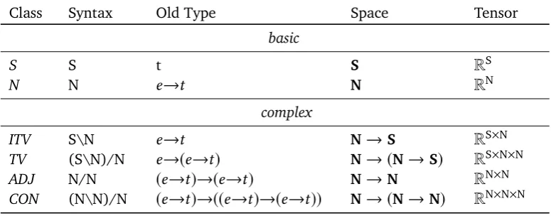
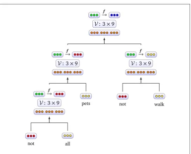
, i.e. expressions are mapped to an object representing both its syntactic structure (essentially, a parse of the expression), and the meaning of the expression, under this parse, expressed in the vector space. It should be easy to see that this mapping resembles the one seen in the symbolic approach, i.e. assigning to each expression a category and a type. Formalizing this intuition is clearly more challenging, and is one of the achievements of Coecke et al. (2010).

Tensor-Based Derivation Table 3.1 is the updated version of Table 2.1, relating

language expressions, syntactic categories (based on a simplistic categorial grammar), the previous interpretation of these expressions as functional types, and the new vector space semantics, i.e. the tensor-based interpretation of the current system. Note that the type-based approach establishes a new correspondence between expressions, syntactic categories and meaning, but that there is not necessarily a full correspondence between old and the new meanings. For example, basic types in the symbolic theories were individuals of type

e

, and truth values of type

t

. We will consider next the reasons for another choice for the basic categories in a vector space setting, i.e. why common nouns are theprimitivesof the new system, rather than being complex types like in the symbolic approach.

category. The composition of expressions, marked here by enclosing the tensors in square brackets, consists in applying thefunctiontensor to itsargumenttensors, where the application process is specified by semantic rules defined in analogy to the syntactic rules. Functional application itself can be implemented in different ways, e.g. by tensor contraction, matrix multiplication, or matrix-vector multiplication, depending on the form the tensors take in a particular model.

3.3.3

Basic Spaces of Models

Similar to thebasic typesof the symbolic approach, certain vector spaces in the typed approach arebasic(or atomic) spaces, as seen in the syntax-semantics interface of Table 3.1.

Sentence Spaces Note first that, in principle, one can follow the symbolic theories

and define a two-dimensional “truth value” space. A suggestion to this effect is worked out in Coecke et al. (2010). However, by doing so, the models lose one of their most interesting properties: the ability to compare sentences on a more fine-grained level than by simple comparison of truth values, i.e. measuringsimilarityof sentences e.g. by spatial distance. As an example, consider that in a binary sentence space, the similarity between sentences “The sun is shining” and “It is rather warm today” is the same as the similarity between “The sun is shining” and “There is no greatest integer” (if the weather statements are true in the model). Since this is usually not a desirable feature, the sentence space is mostly set to be a higher-dimensional space. A proposal to this effect can be seen in Grefenstette et al. (2011). Here, sentences containingtransitiveverbs are represented in spaceN

⊗

N, forNthe space of nouns – also the space of arguments of intransitive and transitive verbs. Sentences based onintransitiveverbs are instead represented in the simple noun spaceNitself. This decision is based on the reasoning that sentences with transitive verbrelate basic concepts (features) across the arguments of the transitive verbs, in contrast to simple (unary)predicationover an argument in intransitive verb sentences. Then, the space for transitive verb sentences should be able to represent this additional structural complexity, i.e. defining it as the tensor product of the individual noun spaces.

Learning Space While the choice of the sentence space is effectively a choice of the

modeloutput space, determining the second atomic space can be seen as a choice of the modelinput space, i.e. the space in whichlearningtakes place primarily. Often, this will be the space ofnouns, since the word class carries substantial lexical meaning, and is comparably ‘simple’, being representable by vectors.

objects of learning: in a first step, noun content is derived, which then becomes the input to the next regression step that learns the content of transitive verbs.

3.3.4

Limitations of Typed Approaches

The type-based approach is characterized by a high formal and conceptual clarity that is possibly unique among the compositional model. At the same time, we can think of several problems affecting it.

Dimensionality Problems The objection relates to theproblem of dimensionality mentioned in Appendix A.0.3, i.e. the intractable nature of higher-order tensors in high-dimensional tasks. Recall that parameter size grows exponentially with the order of the tensor, and that full-rank third-order tensors already are hardly practical in high-dimensional spaces. Note then that the type-based tensors go well beyond third-order: Ditransitive verbs, like ‘give’, are fourth-order tensors, while some prepositions, like ‘with’ in “

x

eats

y

with a

z

”, are fifth-order tensors. Even higher typed expressions

exist, and further complications might arise if the typed approach would incorporate type shifting. The latter is a standard technique in formal semantics, where in cases of type mismatch, the type of an expression can be lifted (raised), possibly further increasing tensor order.

Related to parameter explosion is the problem ofsparsity of data. If learning the word content of tensors would proceed without deconstructing expressions based on them, examples of these expressions would be too infrequent for learning to succeed. Further, their meaning would not be derived correctly – for example, “drinking water” and “drinking wine” would not relate through their common verb. If instead learning methods break apart such expressions, as in the multi-step regression of Grefenstette et al. (2013), data sparsity can be avoided, but higher computational cost is incurred by the iterated learning methods.

The approach can therefore only be made to work iftensor approximationmethods are employed, as seen in Appendix A.0.3. Proposals to this effect exist: Grefenstette et al. (2013) and Polajnar and Clark (2014) use low-rank third-order tensors for transitive verbs. Nonetheless, the dimensionality problem is likely to persist: Third-order tensors can usually be made tractable with dimensionality reduction methods, but tensors of very high order often remain intractable even then.7 _{It seems overly} optimistic therefore to expect that tensors of order five or above will become practically usable in the near future, given the available dimensionality reduction or approximation techniques.

Conceptual Limitations Another point of criticism of the type-based approach

stems from a primarily linguistic concern. The rigorously defined translation of symbolic theories into vector spaces can both be seen as a major advantage, and as a

7 _{While some tensors of very high order can be made tractable due to their structural properties, in}