MoL 2007 02: Discovering the truth by conducting experiments

(1)

Discovering the truth by conducting

experiments

MSc Thesis

(

Afstudeerscriptie

)

written by

Wouter Michiel Koolen

(born July 2nd, 1982 in Groningen, The Netherlands)

under the supervision ofDr. Peter Gr¨unwald, and submitted to the Board

of Examiners in partial fulfillment of the requirements for the degree of

MSc in Logic

at theUniversiteit van Amsterdam.

Date of the public defense: Members of the Thesis Committee: 7th

December, 2006 Prof. Dr. Johan van Benthem Lector Dr. Peter van Emde Boas Dr. Nikos Vlassis

(2)

(3)

Prolusion

Paul Vit´anyi’s 2003 Kolmogorov complexity lecture included a computer

exer-cise in which a polynomial relation had to be learnt from samples.1 _{The following}

data were provided: a sequence of pairs of numbers (h1, d1),(h2, d2), . . . ,(hn, dn),

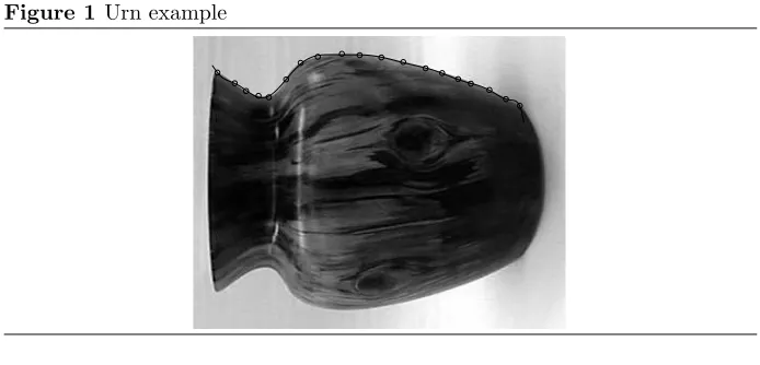
supposedly noisy measurements of a classical urn,hibeing the height from the

floor anddi being the diameter of the urn at the height hi. The goal was to

infer a polynomial that represented the relation between height and diameter. For a given degree, this can easily be done using linear algebra. The crux of the exercise was finding the best degree. An example is shown in Figure 1.

To me, learning from given data is only part of a more general concept of learning, and I started to wonder whether the techniques that I learnt dur-ing my studies could be adapted to an interactive settdur-ing, allowdur-ing the learner to perform experiments. For example, when learning polynomials, the learner could be allowed to choose a point, and she would then receive the value of the polynomial at that point.

[image:3.595.98.445.541.708.2]

For this thesis, I started working on the interactive polynomial learning problem, but it turned out to be much too hard. I then devised the balance scale problem (see Chapter 4), a toy problem that conserves the important features of the polynomial learning problem: it is interactive, probabilistic, model-based, but finite. I had by then developed a slight aversion to subjective Bayesian methods, for my initial work on the polynomial learning problem suggested that they are not robust. It seemed that a subjective Bayesian learner can be tricked into assigning high posterior probability to a certain proposition while

Figure 1 Urn example

(4)

this proposition is false, and additionally, great confidence in this proposition leads to great confidence in the usefulness of experiments that in fact do not help to determine that this proposition is false.

With this in mind, I decided to perform a worst-case analysis of the balance scale problem, and of similar problems in general. This problem naturally de-composed into the truth-finding problem, where we want to find the true model from given data, and the experiment-design problem, where experiments have to be selected, whose outcomes subsequently serve as the data for truth finding. I have yet to solve the balance scale problem completely. But I have already learned and discovered much more than I could initially imagine.

I hope that this thesis will provide inspiration to others.

Wouter Koolen-Wijkstra

Amsterdam

(5)

List of Figures

1 Urn example . . . i

1.1 Example of fit . . . 4

2.1 Examples of unit simplices . . . 13

3.1 Partition of possible worlds . . . 25

3.2 Truth-finding game tree . . . 29

3.3 Convex hull of models . . . 34

3.4 Least favourable distribution . . . 40

3.5 Iso-similarity graphs . . . 44

3.6 K-distance vs KL-divergence I . . . 44

3.7 K-distance vs KL-divergence II . . . 45

3.8 Three types of learning . . . 47

4.1 Balance scale . . . 52

4.2 Two error matrix examples . . . 53

4.3 Experimentation game tree . . . 56

4.4 Bribed jury example . . . 58

4.5 Generalised entropy for Bribed Jury . . . 59

4.6 Balance scale: weight . . . 69

4.7 Balance scale: index . . . 70

(9)

List of Tables

1.1 Example scenarios with hypotheses and models. . . 3

3.1 Biased coin example models . . . 25

4.1 Overview of examples . . . 54

C.1 Notation for sets, pseudo-random variables and elements . . . 80

C.2 Notation and type of important functions . . . 80

(10)

List of Protocols

1.1 The truth-finding game (informal) . . . 6

1.2 The experimentation game (informal) . . . 9

3.1 The truth-finding game . . . 27

(11)

Chapter 1

Introduction

Science progresses by the performing of experiments to evaluate hypotheses.

1.1 Problem statement

This thesis is motivated by two important and interesting questions:

Question 1. How can data be used to learn about reality?

Question 2. How can experiments be used to accelerate learning?

These questions are important, because their answers should provide a solid foundation for rational, e.g. scientific, learning. The answers will most likely also provide new insights into natural, e.g. human, learning. These questions are interesting, because they have not yet been answered satisfactorily, in spite of their importance. Existing approaches require prior knowledge of a specific kind, focus on the learning of predictors, and are mostly analysed in non-sequential settings.

In this thesis, we formalise the first question in the framework of decision

theory as the Nature versus Learner truth-finding game. This game focuses

on finding the true model instead of on prediction. We perform a worst-case analysis of this game, requiring no prior knowledge. We provide the solution to the truth-finding game in the form of optimal strategies for both players, and interpret the value of the game as a measure of certainty.

We formalise the second question as the NatureversusExperimenter

experi-mentation game: a straightforward generalisation of the truth-finding game that includes sequential experimentation. We also solve this game, and compare our solution to that of Bayesian experiment design.

Overview This introduction is structured as follows. We describe the

compo-nents of the learning setting in§1.2, and introduce our two running examples.

In§2.6.1 we explain how information can be quantified. This allows us to

mea-sure how much has been learned. Then in§1.3, we put forward the truth-finding

problem: its interpretation as a game, and the first detailed example. In§1.4 we

(12)

1.2. Basic terminology Chapter 1. Introduction

example. We summarise the contribution of this thesis in §1.5. We conclude

with a list of related work, and words of gratitude.

1.2 Basic terminology

Experiment An experiment is a two-stage act. First, one influences the state of the world in a controlled way, for example by injecting a mouse with a certain

dose of elixir. The action that is undertaken in this first stage is called theinput

of the experiment. Second, one observes the value of a predetermined quantity, for example the lifespan of said mouse measured in days. The value obtained

in this second stage is called the outcome of the experiment. Note that in

controlled experiments, for example clinical trials, one separately observes the outcome that occurs when no influence is exerted. In this thesis, we do not

assume that there is such a specialnull input, but always compare the outcomes

of several experiments. A series of experiments yields data, the concatenation

of successive input/outcome pairs.

Hypothesis A hypothesis provides an explanation for a phenomenon; it

re-lates that what one caninfluence to that what one canobserve. Adeterministic

hypothesis predicts a single outcome for each possible input. A probabilistic

hypothesis assigns a likelihood to each outcome for each possible input. Deter-ministic hypotheses are mathematically represented as functions; probabilistic hypotheses are represented as (conditional) probability distributions. The latter, more general type, will be used in this thesis, as we are interested in modelling phenomena that involve chance. Hypotheses of both types abound in science. We can regard science as the prime application of both learning from data and experimental learning.

In practice, hypotheses are used for different purposes:

• to describe regularities in past experiments,

• to predict the outcome of future experiments, and

• to explain, i.e. formally specify, a data-generating process.

In this thesis, we focus on the third interpretation.

Evaluation Experiments provide the empirical basis for the evaluation of hy-potheses. A deterministic hypothesis can (theoretically) be disqualified on the basis of a single contradictory outcome. It is generally impossible to reject probabilistic hypotheses, but they lose credibility when they predict poorly, i.e., they assign low probability to subsequently observed outcomes of experiments. In the absence of prior knowledge of the generating process, there is no abso-lute quantitative scale to judge prediction quality, hence we can only evaluate prediction quality in comparison to the prediction quality of other hypotheses.

(13)

Chapter 1. Introduction 1.2. Basic terminology

provide no means to combine the specific predictions made by the member hy-potheses into a single prediction. There are ways to achieve such prediction

though, for instance by using aBayesian universal model. This is a model

en-dowed with weights for each member hypothesis. A Bayesian universal model can be translated into a hypothesis, by taking the weighted average of the mem-ber hypotheses.

A collection of models is called competing if no pair of models shares a

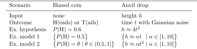
common hypothesis. As an example, consider the following scenarios, which are summarised in Table 1.1.

Scenario 1 (Biased coin). A coiner has just minted a prototype coin showing the new queen’s face. The new queen is rather gourmand, so he wonders whether the coin is loaded. To find out, he can perform experiments by flipping the coin, and observing the side that turns up, either heads or tails. Hypotheses are of

the form: the probability that heads turn up is θ, whereθ is a number between

0 and 1. Models are, for example, the coin is fair (ex. model 1), which is a

singleton set, orthe coin favours heads (ex. model 2), which is an uncountable

set of hypotheses.

Scenario 2 (Anvil drop). Galileo, author of the definitive guide to Earth’s gravity, established that sufficiently heavy objects, when dropped from equal height, hit the ground simultaneously. Now he wants to find out how falling time relates to height. To this end, he has brought an anvil and a stopwatch to the tower of Pisa. He performs an experiment by climbing up to some floor

at heighth, dropping the anvil, and measuring the amount of time t it takes

the anvil to hit the pavement. His hypotheses relate t to h, for example via

the equation h ≈ 4t2_{. (We write} _≈ _{to signify that we use a fixed zero-mean}

noise model. In this case, t = ph/4 +Z, where Z is a normally distributed

random variable with mean zero. The outcome of an experiment, the measured

timet, is noisy; it cannot be obtained exactly due to limited reaction speed and

precision. We approximate the combined influence of such small errors with a normal distribution. Thus, again we use probabilistic hypotheses.)

Models are, for example, linear gravity (ex. model 1) or quadratic gravity

(ex. model 2).

[image:13.595.100.442.635.721.2]

Reality, worlds In this thesis, we use the word reality in a technical sense. It designates a data-generating process, which we cannot identify, but on which we can run experiments. We regard the procedural details of the execution of the experiment as part of reality itself. For example, in Scenario 2, reality is the process that generates a stopwatch reading when provided with a height.

Table 1.1Example scenarios with hypotheses and models.

Scenario Biased coin Anvil drop

Input none heighth

Outcome H(eads) or T(ails) timet with Gaussian noise

Ex. hypothesis P(H) = 0.6 h≈4t2

Ex. model 1 P(H) = 0.5 h≈αt |α∈[1,10]

(14)

1.3. Selection tasks Chapter 1. Introduction

Reality is not necessarily a probability distribution, although we will require this assumption later when we turn to truth finding.

Reality, which we will also callthe state of nature, is unknown to us. We can,

however, consider a collection of candidate explanations of reality: alternative states of nature that we cannot yet distinguish from the actual state. We adopt

the nomenclature of modal reasoning, and call such alternative states possible

worlds. We refer to the current state, reality, as the actual world. Again, in truth finding, we assume that the actual world is a possible world.

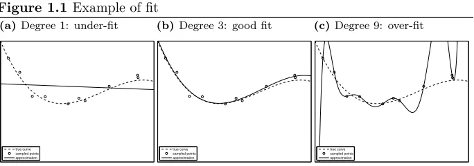
Overfitting Intuitively, a hypothesis over-fits if it describes past outcomes well, but predicts future outcomes poorly. Such a hypothesis is too specific; it describes the noise instead of the regularity in the past outcomes, hence it misses the general pattern. See Figure 1.1 for a graphical example. Ten data-points were generated from the true dotted curve, with Gaussian noise added. The best fitting polynomials of degree 1, 3 and 9 are shown. The under-fitting curve (a) describes the sampled points poorly, and explains the true curve poorly. The

over-fitting curve (c) describes the sampled pointsperfectly, but explains the true

curveextremelybadly. Curve (b) strikes a good balance between descriptive and

explanatory quality.

The statistical literature, e.g. [Mit97], is full of theorems showing that to get good predictive quality, you need to take the hypothesis that optimises some trade-off between complexity and goodness of fit.

1.3 Selection tasks

Learning amounts to finding regularity in data. An elegant formalisation of this

idea is given by the theory of Kolmogorov complexity, where all computable

regularities are considered. See [LV93] for an introduction to the field. The Kolmogorov complexity itself is not computable.

To obtain a computable notion of regularity, one must restrict the class of regularities under consideration. Such restrictions lie at the heart of minimum description length (MDL) methods, see [GMP05]. As in MDL, we use models to explicitly state which regularities are considered.

[image:14.595.153.495.590.710.2]

The following question is a more precise formulation of Question 1:

Figure 1.1 Example of fit

(a)Degree 1: under-fit

true curve sampled points approximation

(b)Degree 3: good fit

true curve sampled points approximation

(c)Degree 9: over-fit

(15)

Chapter 1. Introduction 1.3. Selection tasks

Question 3. Given a sequence of data obtained from reality and a list of reg-ularities, how can we infer the best explanation for reality on the list, i.e. learn something about it?

We list three answers to Question 3, that differ in the precise interpretation of “best explanation”: hypothesis selection, model selection, and truth finding. But first we make the following observation about selection methods on probabilistic objects in general.

Probabilistic humility The general principle

probabilities in⇒probabilities out (PIPO)

states that, once a problem has been formalised in probability theory, then reasoning within probability theory can only yield the probability of new events. The goal of model selection is to find the best model. By PIPO, probability theory can only give us a probability distribution on the candidate models. We need an additional criterion, outside of probability theory, to judge the quality of such distributions. The same holds for hypothesis selection and truth finding.

Hypothesis selection The hypothesis-selection problem is stated as follows:

given a collection of hypotheses and data obtained from reality, find the hypothe-sis that explains reality best. Of course, one cannot evaluate directly how well a hypothesis explains reality, one can only evaluate how well it describes the data. To guard against over-fitting, one must select a hypothesis that strikes a balance between expressiveness and simplicity. This can be achieved by (1) adopting a measure of complexity for hypotheses, and (2) penalising hypotheses by their complexity. For example, in Figure 1.1, we penalise polynomials according to their order. This ensures that we prefer (b) over (c).

The hypothesis-selection problem between two hypotheses is called

hypoth-esis testing. To obtain a true selection, beyond PIPO, one uses a significance level as a selection threshold.

Model selection The model-selection problem is the following: given a collec-tion of models and data obtained from reality, find the model that explains reality

best. This problem is often solved by reducing it to the hypothesis-selection

prob-lem using universal codes. A universal code for a model corresponds to asingle

hypothesis, composed of a weighted average over the partaking hypotheses. Two well-known approaches are Bayesian and MDL model selection, see [GMP05].

Truth finding The truth-finding problem is the following: given a collection of competing models and data obtained from reality, find the true model. We regard the hypotheses in the models as possible worlds, and assume that one of

them is reality. The model that contains reality is called thetrue model, and

we want to obtain as much information about its identity as possible. Selecting a single model with certainty is generally impossible, because we are working with probabilistic hypotheses. We allow a more general answer: a probability distribution on models, which expresses any remaining uncertainty about the true model. The performance of such a distribution is evaluated by the

(16)

1.3. Selection tasks Chapter 1. Introduction

Quantifying information The truth-finding problem is different from the preceding two problems, for it makes the additional assumption that reality is in one of the models. The availability of a true model allows a natural measure of

errororloss, namely the amount of information that we, the learner, lack about this true model. To measure this amount, consider the following hypothetical situation. Suppose that there is a helpful external observer that knows which model is true. This observer sends us a message (e.g. an SMS), to tell us which

model is true. The more information we already possess about the true model,

the shorter this message needs be. We equate the amount of information that we lack about the true model with the length of the shortest message that will make us totally informed about the true model.

Log loss The above sending of messages is formalised in information theory using codes. Codes allow us to measure message lengths in bits. Throughout this thesis, we will use probability distributions as mathematical generalisations of codes. A probability distribution can be regarded as a code with idealised (non-integer) code-lengths. This correspondence will be explained in more detail

in §2.6.1. Let P be the distribution on models that represents our uncertainty

about the true model, i.e. that we use as a code, and letM∗_{be the true model.}

Then the amount of information that we lack aboutM∗_{, denoted}_L

logand called

thelog loss, is given by

Llog(P,M∗) =−logP(M∗). (1.1)

Minimising the log loss is equivalent to maximising the probability that we assign to the true model. Of course, we — the learner — cannot determine the log loss ourselves, because we do not know the true model.

We stress that the distribution P on models that is learned can always be

interpreted as a code. Only in special situations can the probabilities that P

assigns to the models be interpreted as their relative frequencies of occurrence, or as the learner’s subjective degree of belief in their truth. We describe these

situations in§3.7.4.

Truth-finding game To analyse the truth-finding problem with log loss, we

formulate it as a game. Thetruth-finding game, a strictly competitive game with

chance moves, is played between the players Learner, Chanceand Nature. The

arena of the truth-finding game is a set of competing models. Naturepicks the

world that generates the data from one of the models,Chanceactually generates

the data, andLearner tries to gain as much information as possible about the

true model using the data. The entire game is shown in Protocol 1.1.

Protocol 1.1The truth-finding game

Arena: Competing modelsM={M1,M2. . .}.

Require: Number of outcomes n.

1: Naturecovertly chooses a hypothesisθ∗_{. Say}_θ∗ _{is in model}_M∗_. 2: Chancesamples a sequence of outcomesy1, y2. . . yn fromθ∗.

3: Learner expresses his belief as a probability distributionP on models.

(17)

Chapter 1. Introduction 1.3. Selection tasks

Example 1.1(Biased coin). The following is a run of the truth-finding game

for Scenario 1. We start with two models: fair coin, and coin favours heads.

Formally, we haveM={M1,M2}, where

M1=P(H) = 0.5 fair coin

M2=P(H)∈[0.6,1] coin favours heads

We have slightly altered the definition of the second model in this example for illustrative purposes. This version of the biased coin scenario will be called

Reduced Biased Coin in Chapter 3, where we continue this example. Sayn, the

number of coin flips we will perform, is fourteen. NowNaturestarts by choosing

a world from either of the models. Say she picks the coin with bias 0.6, from

the second model. This means that, for the rest of this game, model two is the

true model. (This simple strategy forNatureis not optimal. The best (minimax

optimal) strategy is given in Chapter 3.) ThenChancegenerates 14 outcomes

of the coin with bias 0.6. Say these are the outcomes:

H,T,H,H,H,T,T,T,H,H,H,T,T,H

Finally, Learner must express his belief about the true model as a probability

distribution on models. He does not know which model is true, but he has seen the outcomes. Disregarding the order of the outcomes, he could just count:

6×T and 8×H. Now, following the worst-case-optimal strategy described in

Chapter 3, he produces the following probability distribution on models:

P(M1) = 0.4701 P(M2) = 0.5299

Note thatLearneronly slightly favours the second model. This a cautious choice,

because the data are not very informative. Then the true modelM2is revealed,

and the information thatLearnerlacks about this model is computed using the

log loss. It is given by −logP(M2) = 0.9162. Our analysis will show that

the expected loss forLearner, using the worst-case-optimal strategy is 0.9040.

The current loss is higher, but this is not due toNature, but to Chance. The

outcome, whichChancegenerated at random, is just not very informative.

Worst-case-optimal strategy In this thesis we analyse the truth-finding game from a worst-case perspective. That is, we search for a learning procedure, a strategy, that constructs a probability distribution on models from observa-tions, such that, using this procedure, we gain as much information about the true model as possible, in the worst state of nature for this particular proce-dure. The motivation for this approach is that it gives the best performance guarantees if we are not prepared to make further assumptions.

To evaluate a strategy, we compute its risk. This is the mean loss that the

learner obtains using this strategy, where the average is taken over allChance’s

moves. The risk of a strategy does depend onNature’s move, but no longer on

Chance. Then, taking the worst-case-optimal strategy forLearner, we eliminate

dependence onNature. Therefore, the worst-case-optimal strategy and its risk

require no assumptions aboutNature. One of the models has to be true, but, in

(18)

1.4. Experiments Chapter 1. Introduction

Worst-case belief Worst-case analysis is quite different from Bayesian anal-ysis. In the latter, it is assumed that the learner can always construct a proba-bility distribution on possible worlds, expressing his prior uncertainty about the actual world. The crucial difference is that the Bayesian learner uses this dis-tribution for two purposes. First, he selects the act that is optimal with respect to this distribution. Second, he assesses his own performance with respect to

this distribution, using it as though it weretrue. We think that this approach

is essentially circular.

It is interesting that our worst-case analysis also constructs a probability distribution on possible worlds. This probability distribution can be interpreted as the prior belief that the learner should have about the true model, in the

sense that it is a worst-case-optimal mixed strategy for Nature. For Learner,

believing this distribution is not problematic; if it is not true, thenNaturedoes

not play optimally, and the incurred risk for Learner can only decrease. The

constructed probability distribution on models depends heavily on the structure of the models, and is often particularly non-uniform. This directly contradicts Bayesian philosophy, which, taken in a weak form, prescribes the assumption of a smooth, fairly uniform, distribution, in the absence of specific prior knowledge.

1.4 Experiments

We now address the task of truth finding when we can perform experiments.

Experiment design The experiment-design problem is the following: given a collection of competing models, perform the experiments that, in the end, yield most information about the true model. We allow experiments to be chosen sequentially, this means that we can choose the next experiment based on the data obtained in all previous experiments. Example 1.2 is provided below as an illustration.

Previously, hypotheses were probability distributions on outcomes. In exper-iment design, hypotheses are conditional probability distributions on outcomes given input. Here, the input is the experiment selected by the learner. The true hypothesis fixes the way experiments work, by dictating the probability of each outcome for each input.

The experiment-design problem can be seen as experiment selection followed by truth finding. The data used for truth finding are the outcomes of the selected experiments. The task of experiment design amounts to choosing an experimentation strategy to maximise the amount of information that truth finding obtains.

To analyse the experiment-design problem, we translate it into a game.

Experimentation game The experimentation game, a strictly competitive

game with chance moves, is played between the players Experimenter, Chance

and Nature. The experimentation game extends the truth-finding game with

experiments. This extra ability forLearnerlicenses his new name: Experimenter.

A run of the game proceeds as follows. Nature initially picks the world in

which all experiments take place. ThenExperimenterchooses an experiment, and

(19)

Chapter 1. Introduction 1.4. Experiments

times, allowing Experimenterto base his choice on previous outcomes. Finally,

Experimenter is evaluated as in the truth-finding game. He must provide a probability distribution on models, and suffers the log loss, that is, the amount of information this distribution lacks about the true model. The experimentation game is summarised in Protocol 1.2.

Protocol 1.2The experimentation game

Arena: Competing modelsM={M1,M2, . . .}.

Require: Number of experimentsn.

1: Naturecovertly chooses a hypothesisθ∗_{. Say}_θ∗ _{is in model}_M∗_.

2: fornturnsdo

3: Experimenterchooses an experiment inputξ.

4: Chancegenerates an outcome as predicted byθ∗ _on_ξ_. 5: end for

6: Experimenterexpresses his belief as a probability distributionP on models.

Loss: Experimentersuffers−logP(M∗_).

Example 1.2(Anvil drop). The following is a run of the experimentation game

for Scenario 2. We start with two models: linear gravity andquadratic gravity.

Formally, we haveM={M1,M2}, where

M1=h≈αt |α∈[1,10] linear gravity

M2=h≈αt2|α∈[1,10] quadratic gravity

The tower of Pisa has six galleries. Correcting for inclination, the first one is located at the height of four metres above the tower base. Each next one adds

another four metres of height. Experimenter, Galileo, drops an anvil by gently

pushing it over the edge of a loggia.

First Naturechooses the actual world; suppose she choosesh≈5t2_{. More}

precisely, this means t ∼ ph/5 +ǫ, where ǫ is Gaussian noise with variance

0.1. This fixes quadratic gravity as the true model for the rest of the game.

Historical fiction1 _{tells us that Galileo dropped two heavy objects from the}

tower. We adopt this number of experiments. Say the first anvil is dropped

from the topmost gallery, h= 6·4 = 24. Then Chancegenerates an outcome

according toh≈5t2_{, say}_t_{= 2}_._{2 seconds. Now}_Experimenter_{can choose another}

experiment, say he drops the second anvil from h = 3·4 = 12, and Chance

generatest= 1.6.

It now remains to perform the evaluation step, which continues exactly as in the truth-finding game. The data, the concatenation of successive in-put/outcome pairs, are

h24,2.2i,h12,1.6i

1_{This story, although reported by Galileo’s own student, is widely considered to be a legend}

(20)

1.5. Contribution of the thesis Chapter 1. Introduction

1.5 Contribution of the thesis

Truth-finding2 _{is, to the best of our knowledge, a new way to formalise the}

learning problem. Its prime motivations are the following.

• Models are the interesting level of abstraction for learning.

• Worst-case analysis is a good answer to the absence of prior information,

as it provides rigorous bounds without further assumptions.

We provide the worst-case solution of the truth-finding game, in the form of a procedure to find the worst-case-optimal strategy. We give an algorithm, and prove that it finds the worst case optimal strategy. As already described, this procedure constructs a probability distribution on possible worlds, and then acts optimally with respect to this distribution. One might say that this probability

distribution isobjective, as it is induced by the structure of the game, and not

based on the learner’s judgement.

The second half of this thesis is devoted to experiment design. We use truth finding as a building block, and hence adopt its motivations. We add the following

• Experiments are performed sequentially.

There is considerable literature on Bayesian experiment design, but most of the literature covers a setting in which all experiments are performed simultaneously. See [CV95] for an overview. The sequential setting is, of course, more powerful. There also literature on frequentist experiment design, for example [Puk93]. Also here, there is a focus on performing experiments simultaneously. Other than that, it is not clear how this approach is related.

Theorems 2.30, 2.31 and 3.41 are more minor contributions. The last the-orem is both interesting and simple to prove; we suspect it is not new, but we could not find a published statement of this result.

Related work

Information theory is covered in [CT90], game theory in [Bin91]. Decision theory is covered in the classical [Fer67]. Non-Bayesian experiment design is covered in [Puk93], which focuses on linear models. [CV95] reviews the current state of Bayesian experiment design, while [SW00] compares Bayesian experiment design to Maximum Entropy Selection. The relation between Bayes acts and the Max-imum Entropy Principle is treated in detail in [GD04]. MinMax-imum Description Length model selection is covered in [GMP05].

Organisation of the thesis

Chapter 2 provides notions and results that will be used later. It also serves to introduce our notation and conventions. Among other things, Chapter 2

2_{The term}_{truth finding}_{already has a legal meaning, and it has also been defined as a desirable}

(21)

Chapter 1. Introduction 1.5. Contribution of the thesis

introduces the relevant strategic game theory that allows us to analyse and solve the games in later chapters.

Chapter 3 addresses the problem of truth finding. It provides an analysis and solution of the truth-finding game. It also addresses the problem that there often is no analytical solution, and provides a numerical solution to a simple example.

Experiment design is covered in Chapter 4, where we analyse and solve the experimentation game. Chapter 5 concludes and provides a list of directions for future research.

Acknowledgements

I would like to express my gratitude to the people that made this work possible, both the research and this document. I want to thank Sir´ee Koolen-Wijkstra, my lovely wife, for all her care and love, and for the huge amount of time she invested in my thesis. And I have to say that her massage is unsurpassed.

I was encouraged, inspired challenged and coached by my colleagues at CWI:

Peter Gr¨unwald, Steven de Rooij and Tim van Erven. Their sustained

enthu-siasm and support made doing research and writing this thesis an extremely pleasant experience.

I am grateful to Tikitu de Jager for his thoroughly pedantic proofreading.

A native English speaker with his LA_{TEX expertise, understanding of Dutch,}

(22)

Chapter 2

Preliminaries

This chapter covers the notions and results needed for the development of the theory of truth finding and experiment design in Chapters 3 and 4. This chapter

does not contain new material, with the exception of §2.6.3; it is intended as

a reference, and serves to introduce notation. Readers that are familiar with some of the areas of research described herein may skip these without difficulty, because standard notation has been used wherever possible.

2.1 General notation

We denote byNandRthe sets of natural and real numbers. Both contain 0. The

extended real numbers are defined byR:= [−∞,∞] =R∪ {−∞,∞}, and they

are endowed with the intuitive order and the corresponding order topology. R+

is the set of non-negative real numbers. R++ is the set of positive real numbers.

As usual, Rn is then-fold Cartesian product of R. We use log for the binary

logarithm. It is convenient to regard log as a function fromR+toR, by defining

log 0 :=−∞.

2.2 Set theory

Notation 2.1. Let Φ and Ω be sets. We denote the power set of Ω by

℘

(Ω).

The identity function on Ω is denoted by1Ω. We denote by [Ω→Φ] the set of

all functions from Ω to Φ. We abbreviatef ∈[Ω→Φ] tof : Ω→Φ. We write

f : Ω։Φ iff is a surjective function from Ω to Φ.

Notation 2.2. Let Φ be a set,I a well-ordered set of indices, and Ωi ⊆Φ for

eachi∈I, with duplicates allowed. We denote the functioni7→Ωi byhΩiii∈I.

We call a function of this form anI-familyor anI-sequence.

Definition 2.3. Let Φ be a set. We denote by Φ∗ _{and Φ}<ω_{the set of all finite}

sequences over Φ. We denote by Φω_{the set of all infinite sequences over Φ.}

Definition 2.4. Let f : Φ×Ω →Ψ. For all x∈ Φ, we denote byf(x,·) :=

(y, f(x, y))|y∈Ω . Clearly,f(x,·) : Ω→Ψ. The functionf(x,·), viewed as

a function ofx, is called theSch¨onfinkelisationorCurryingoff. We analogously

(23)

Chapter 2. Preliminaries 2.3. Linear algebra

Definition 2.5. Let Ω be a set. A set Φ⊆

℘

(Ω) is called apartitionof Ω if

1. SΦ = Ω. (Φ covers Ω.)

2. ∅ 6∈Φ.

3. Ψ∩Θ = ∅ for all different Ψ,Θ ∈ Φ. (The elements of Φ are pairwise

disjoint.)

2.3 Linear algebra

Whenevernis clear from the context, we denote by0and1the zero and unity

vectors inRn, i.e. the vectors that have all entries set to either zero or one. For

1 ≤i ≤n, ei is the unit vector of dimension i. We denote the transpose of a

vectorpbypT_.

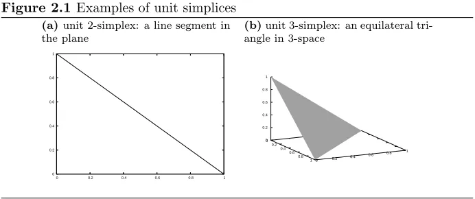
Definition 2.6. Theunitn-simplexis the set given by

∆n:=

n

p∈Rn₊|pT1= 1o.

It is also called thestandardn-simplex orprobability n-simplex. One can

equiv-alently define ∆n as the convex hull of {e1, . . . ,en}. Note that we number the

unit simplices by the number of partaking unit vectors, whereas some other

authors number by dimension (which isn−1), or equivalently include the zero

vector in the convex hull definition.

Each discrete probability distribution on a set ofn outcomes can be

repre-sented by a point in ∆n and vice versa. The unit 2- and 3-simplices are shown

in Figure 2.1.

2.4 Convex analysis

All sets in this section are subsets ofRn. A setC is convex if it is closed under

linear interpolation. We denote by conv(Ω) the convex hull of the set Ω, i.e. the intersection of all convex sets that contain Ω. The convex hull operation preserves openness, closedness and boundedness, hence also compactness.

[image:23.595.99.445.577.722.2]

The following results can be found in a standard textbook on convex opti-misation, for example in [BV04].

Figure 2.1 Examples of unit simplices

(a)unit 2-simplex: a line segment in

the plane

0 0.2 0.4 0.6 0.8 1

(b)unit 3-simplex: an equilateral

tri-angle in 3-space

0 0.2

0.4 0.6

0.8

1 0 0.2 0.4 0.6 0.8 1 0

(24)

2.5. Probability theory Chapter 2. Preliminaries

Theorem 2.7(Supporting Hyperplane Theorem). For every convex setC, and

pointxon the border ofC, there is a hyperplaneP throughx, such that C is

contained in one of the half-spaces ofP.

Theorem 2.8(Separating Hyperplane Theorem). LetH andKbe convex sets

inRn with disjoint interior. Then there exists a hyperplanex|aT_x₌_b _that

separatesH andK.

Theorem 2.9. If f : R2 →Ris convex in (x, y), andC a convex non-empty set, then the function

g(x) = inf

y∈Cf(x, y)

is convex inx, providedg(x)>−∞for somex.

2.5 Probability theory

Probability theory deals with probabilities of events, that is, sets of outcomes. A rigid formalisation of probability theory using measure theory is given in

Appendix A. For the current exposition, it suffices to define aprobability

dis-tribution as a function that assigns probabilities, i.e. numbers from [0,1], to events, obeying certain conditions. We abbreviate probability distribution to distribution whenever convenient.

Throughout this thesis, we will use three standard types of event sets,

de-pending on the type of the set of outcomesX as follows:

• IfX is finite, we use the events

℘

(X).

• If X ⊆ R, we use the events Bor(R). This is the Borel σ-algebra on R,

i.e. the smallest set of events that contains all open sets ofR, and that is

closed under complements and countable unions. If X ⊆Rn, we use the

events Bor(Rn).

• If X is a set distributions on a finite set of size n, we identify it with

∆n⊂Rn, and use the Borelσ-algebra on the latter.

Note that in all cases, the singleton sets ofX appear in the event set.

Definition 2.10. A pairhX,Σi, whereX is a set of one of the above categories,

and Σ is the corresponding set of events, is called asample space. Because Σ is

always clear from the context, we identify a sample space with its carrierX.

Definition 2.11. For any sample space X, we denote by D(X) the set of all

probability distributions onX.

So far, we have not assumed any structure on the set of outcomes X. The

most straightforward way to obtain structure is to use the available structures

on R by assigning real numbers to outcomes, thereby transforming the set of

outcomes into a subset ofR.

Definition 2.12. A functionX :X →Ris called arandom variable. We say

(25)

Chapter 2. Preliminaries 2.5. Probability theory

Sometimes, it is useful to translate the set of outcomes into some set different

fromR. We call such transformationspseudo random variables.

As was just stated, a random variable transforms outcomes into real num-bers. Via this transformation, we can forget about the original distribution, and

consider the induced distribution onR.

Notation 2.13. If a random variableX is distributed according toP, we write

X ∼P.

Definition 2.14. LetX be a random variable defined on the sample spaceX

with distributionP. We define theexpected valueorexpectationofX by

E [X] :=

Z

X

XdP

Definition 2.15. LetX be a random variable on the sample spaceX. We say thatX isconstantif∃c∀x∈ X :X(x) =c. We callX almost surely constantif

∃c:P(X=c) = 1. This impliesP(X= E [X]) = 1.

Remark 2.16. A random variableXonX is almost surely constant if all measure

ofP is assigned to a region whereX is constant. This can be solely due toX,

namely whenXis constant, or solely due toP, namely whenP puts all measure

on a single point, or partially due to both.

Theorem 2.17 (Jensen’s Inequality [Wil91, Theorem, p. 61]). Let X be a

convex set, P a probability distribution on X. Then for any convex function

f :X →R,

EP

f(X)≥f EP[X]

(2.1)

Moreover, if f is strictly convex, then equality in (2.1) implies that X is an

almost surely constant random variable.

One level of abstraction higher, we work with a meta-distribution on sets of probability distributions. We can interpret such a meta-distribution as a prior probability; one first samples a distribution according to this meta-distribution, and then generates an outcome according to the sampled distribution. For more detail, see [GD04, Section 9.2]. Such a meta-distribution can be collapsed into a single distribution on outcomes as follows.

Definition 2.18. LetX be a set,Qa convex set of distributions onX, andQ

a distribution onQ. We define EQ[Q], theexpected distribution ofQonX, by

EQ[Q] (A) := EQQ(A)=

Z

Q

Q(A) dQ

whereQ=1Q is a pseudo random variable, andAany event ofX.

Definition 2.19. LetX, Y be pseudo random variables with rangesX andY.

The distribution P that gives the distribution of the pair hX, Yi is called the

joint distributionofX andY. Themarginal distributionsofX,Y are given by

PX(EX) :=P(EX× Y)

PY(EY) :=P(X ×EY),

(2.2)

for eventsEX andEY overX andY. We writeP(EX) forPX(EX) andP(EY)

(26)

2.6. Information theory Chapter 2. Preliminaries

Definition 2.20. Letnbe the number of outcomes, and letP be a probability

distribution on a countable space. Then-fold product distributionofP, denoted

Pn_{, is given by}

Pn₍_y

1, . . . , yn) := n Y

i=1

P(yi)

2.6 Information theory

Information theory exploits the relationship between probability distributions and codes. In this section, we restrict attention to probability distributions on a finite or countable set. The proofs of the theorems that we merely state below can be found in [CT90].

2.6.1 Quantifying information

Bits and codes

A bit is a variable that ranges over two values. These values can have many

interpretations, for example: on/off, high/low, 0/1 and true/false. In general, a single bit allows one to distinguish between two arbitrary possibilities. To

distinguish between more than two possibilities, one uses acode: a collection of

code words, sequences of bits, with an interpretation for each code word. We restrict attention to codes with the following properties:

• Prefix-free. A code is prefix free if no codeword is a prefix of another. A

non-prefix-free code has two code words a, bsuch thatb extends a. Such

a code uses both the content and the length of code words to convey

information. Such a code is ambiguous; upon receiving, bit by bit, code

worda, one cannot tell whether the message has ended and isa, or whether

it will continue, actually beingb.

• Irredundant. A code is irredundant if no two code words have the same interpretation. A code that has two code words with the same interpreta-tion is obviously inefficient, because code words can only be used one at a time.

• Complete. A code is complete if addition of any new code word renders it non-prefix-free. A code that remains prefix-free when a new code word is added does not use its full potential.

We will henceforth simply use the word code for an irredundant complete prefix-free code.

Codes are used to quantify the information content of objects: the amount of information a certain object contains, with respect to a given code, is given by the length of the shortest code word that is interpreted as this object.

Idealised bits and probability distributions

(27)

Chapter 2. Preliminaries 2.6. Information theory

Theorem 2.21(Kraft Inequality [LV93, p.74]). Letℓ1, ℓ2, . . .be a finite or

infi-nite sequence of natural numbers. There is a prefix-free code with this sequence as lengths of its binary code words iff

X

i

2−ℓi _≤₁_.

Moreover, a code is complete iff this holds with equality.

Consequently, a code on X with code wordsw1 forx1,w2 for x2, etc.

cor-responds to a probability distributionP withP(xi) = 2−ℓi, whereℓi=|wi|is

the length, in bits, of code wordwi. Note that this correspondence does not use

the content of code words, only their lengths.

The inverse of this transformation transforms an arbitrary probability

dis-tribution onX into a list of code word lengths as follows

ℓ1=−logP(x1), ℓ2=−logP(x2), . . .

These code word lengths can be non-integral. We call such numbersidealised

code lengths, and their unit idealised bits.1

This mathematical generalisation gives us a much more fine-grained way to measure the information content of objects: the amount of information that a

certain objectxcontains, with respect to a probability distributionP, is given

by−logP(x). Conversely, we say that this is the amount of information that

P lacks about x.

2.6.2 Basic coding

In the following definitions we use the convention, based on continuity

argu-ments, that 0 log0_q = 0 and plogp₀ = ∞ for p > 0 and all q, see [CT90]. It

follows thatplogp_q =plogp−plogqeven whenq= 0.

Entropy

Definition 2.22. LetX∼P. Theentropy ofX is defined by

H(X) := EP−logP(X) (2.3)

The entropy of X equals the expected codelength, when the outcome X is

encoded using its source distribution P as the code. When P is a distribution

onX, we abbreviateH(1X) toH(P).

Definition 2.23. Theconditional entropy of Y givenX =xis defined by

H(Y|X =x) := E

Y∼P(·|X=x)

−logP(Y|X =x). (2.4)

Theexpected conditional entropy ofY given X2_{is given by}

EXH(Y|X)= EX,Y−logP(Y|X). (2.5)

1_{An important technique in information theory called the}_{Shannon-Fano code}_{allows us to find}

code wordsw1, w2, . . .such that⌈ℓi⌉,ℓirounded up, equals|wi|. A second technique, called

arithmetic coding, allows us to actually achieve these idealised code lengths when we code a sequence of objects, even when a different probability distribution is used for each object.

2_{In [CT90], the expected conditional entropy is abbreviated to}_H₍_Y_|_X_{). We cannot adopt this}

(28)

2.6. Information theory Chapter 2. Preliminaries

Theorem 2.24(Chain Rule of Entropy).

H(X, Y) =H(X) + EXH(Y|X). (2.6)

KL-divergence

Definition 2.25. For distributionsP, Q, we define theKullback-Leibler diver-genceofQfromP by

D PkQ:= EP

logP(X)

Q(X)

(2.7)

= EP

−logQ(X)− H(P). (2.8)

The Kullback-Leibler divergence of Qfrom P is the number of additional bits

one expects to use when coding an outcome fromP usingQinstead ofP.

Note that D is not symmetric inP andQ, so it is not a distance. It does

however have the following important property.

Theorem 2.26(Information Inequality). LetP, Qbe probability distributions. Then

D PkQ≥0 (2.9)

with equality iffP=Q.

This means that, in expectation, the best code for outcomes that are

gener-ated fromP, isP itself.

Theorem 2.27. LetPn_,_Qn _{be product distributions. Then}

D(Pn_k_Qn_{) =}_n_D₍_P_k_Q_{) and} _H₍_Pn_{) =}_n_H₍_P₎_.

Proof. It suffices to show

E

Yn_∼_Pn

logQn(Yn)= E

Y1∼P

· · · E

Yn∼P

logQ(Y1) +· · ·+ logQ(Yn) (2.10)

= E

Y1∼P

logQ(Y1)

+· · ·+ E

Yn∼P

logQ(Yn)

(2.11)

=n E

Y∼P

logQ(Y), (2.12)

the rest is just definition chasing.

Theorem 2.28. D PkQis convex in the pair (P, Q), that is, for all

distribu-tionsP1, P2, Q1, Q2and for all 0≤λ≤1 we have

D λP1+ (1−λ)P2kλQ1+ (1−λ)Q2 ≤ λD P1kQ1+ (1−λ)D P2kQ2

Mutual information

Definition 2.29. For random variablesX andY with joint distributionP and

marginal distributions PX andPY, we define the mutual information between

X andY by

I(X;Y) := EP

log P(X, Y)

PX(X)PY(Y)

(2.13)

=D(PkPXPY) (2.14)

=H(X) +H(Y)− H(X, Y) (2.15)

(29)

Chapter 2. Preliminaries 2.6. Information theory

2.6.3 Advanced coding

We analyse three somewhat advanced coding scenarios.

Conditional coding

The following theorem is a generalisation of the information inequality. Suppose

that a pair of outcomesX, Y is generated fromP, and we are first toldX =x,

and then need to encodeY. Then the best code for this, again in expectation, is

the conditional distributionP(Y|X=x). Of course, this conditional probability

is not defined when P(X =x) = 0, but then simultaneously, the probability

that we observexin the first place is zero.

Theorem 2.30(Generalized Information Inequality). LetX andY be sample

spaces, and letP, Q be probability distributions overX × Y. Then

EP−logP(Y|X)≤EP−logQ(Y|X) (2.16)

with equality if and only if P(Y|X) = Q(Y|X) almost surely. Here, almost

surely means wheneverP(X)>0.

Proof. For allxs.t. P(x)>0, we have, by the Information Inequality,

EY|x

−logP(Y|x)≤EY|x

−logQ(Y|x), (2.17)

with equality iffQ(Y|x) =P(Y|x). Taking the expectation overP(X) in (2.17)

yields (2.16), observing that the xwhere P(x) = 0 do not contribute to the

expectation at all. This immediately shows that equality holds iff P(Y|X) =

Q(Y|X) almost surely.

Meta-coding

Suppose we have a meta-distribution on codes, that we want to use to encode an

outcome fromP. We can either sample a code from our meta-distribution, and

then use that to encode the outcome, or we can encode the outcome with the expected code. The following theorem proves that, in expectation, the latter is better.

Theorem 2.31. Let X be a set, and Q a convex set of distributions on X.

Then for all distributionsQonQandP onX:

EQ

D(PkQ)≥ D(PkEQ[Q]). (2.18)

Proof. First, observe that (2.18) holds iff

EQEP

logP(X)

Q(X)

≥EP "

log P(X)

EQQ(X)

#

(2.19)

iff EPEQ−logQ(X)≥EP

h

−log EQQ(X)i (2.20)

Second, note thatfx :Q → [0,∞] defined by fx(Q) :=−logQ(x) is a convex

function (ofQ) for allx∈ X. Application of Jensen’s Inequality (2.1) yields:

EQ

fx(Q)≥fx(EQ[Q]) so EQ

−logQ(x)≥ −log EQ

Q(x)

(30)

2.7. Game theory Chapter 2. Preliminaries

Conditional meta-coding

The next theorem generalises the previous theorem to the case where P is a

joint distribution onX, Y, and we need to encodeY given thatX =x.

Theorem 2.32. LetX, Y be sets, andQa convex set of conditional

distribu-tions onY givenX. Then for all distributionsQonQand P onX × Y:

EPEQ

−logQ(Y|X)≥EP h

−log EQ

Q(Y|X)i. (2.21)

Proof. The proof is analogous to that of Theorem 2.31, using the convex function

fx,y(Q) :=−logQ(y|x) instead.

2.7 Game theory

Definition 2.33. A tripleG =hSA, SB, πiis called a matrix gameifπ:SA×

SB →R. A matrix game is a two-player zero-sum game in strategic form. We

call the elements ofSA and SB pure strategies for players A and B, andπ the

payoff.

Definition 2.34. We define the minimaxvalue V andmaximin value V by

V := inf

sB∈SB sup

sA∈SA

π(sA, sB) (2.22)

V := sup

sA∈SA inf

sB∈SB

π(sA, sB) (2.23)

These value can be interpreted as follows. The maximin value (supposing that the supremum is attained) is the highest payoff that player A can guarantee, when player B chooses her move after learning the move of player A. Similarly, the minimax value is the least payoff that player B can guarantee when her move is reported to player A before he has to choose his move.

If V = V, we call this quantity the valueofG and denote it by just V. If a

game has a value, thenplaying second provides no advantage.

Remark 2.35. Always V≤V, but not necessarily V = V.

Definition 2.36. We call (˜sA,s˜B) asaddle-pointof πif for allsA, sB

π(˜sA, sB)≥π(˜sA,s˜B)≥π(sA,˜sB).

The existence of a saddle-point guarantees that G has a value. On the other

hand,G may have a value but no saddle point. This occurs when the infimum

is not a minimum in (2.22), or the supremum is not a maximum in (2.23).

Definition 2.37. LetG be a matrix game. We call ΣA :=D(SA) and ΣB :=

D(SB) themixed strategiesfor players A and B. We lift the pure strategy payoff

πto the mixed strategy payoff Π : ΣA×ΣB→Rby

Π(σA, σB) :=_s E

A∼σA

sB∼σB

π(sA, sB)

:= Z

SA×SB

(31)

Chapter 2. Preliminaries 2.7. Game theory

We callGe:=hΣA,ΣB,Πithemixed matrix game generated by G. Its minimax

value V and maximin value V are given by

V := inf

σB∈ΣB sup

σA∈ΣA

Π(σA, σB) (2.24)

V := sup

σA∈ΣA inf

σB∈ΣB

Π(σA, σB) (2.25)

Theorem 2.38(Minimax Theorem [Bin91, Theorem 6.4.4]). IfG=hSA, SB, πi

is a matrix game with compact setsSA and SB and continuous payoff π, then

V = V forGe.

Corollary 2.39. LetG=hSA, SB, πibe a matrix game, withSAandSBfinite,

then V = V forGe.

Definition 2.40. A pairhT, <iis a treeif

• <is a strict partial order onT, i.e. irreflexive, antisymmetric, transitive,

• there is a unique<-least element, and

• for eachx∈T,y∈T |y < x is well-ordered by<.

As usual, we shall useT to refer tohT, <i. The<-maximal elements are called

terminalsorleaves ofT, the other elements are callednon-terminals. The sets

of leaves and non-terminals are denoted lf(T) and nt(T). The unique <-least

element ofT is called therootofT.

Definition 2.41. Agame treeis a sextuple D

T, <, A, m,hMti_t_∈_T,hIai_a_∈_A,hπai_a_∈_A E

where the following conditions hold:

• hT, <iis a finite tree. We call the elements ofT positions.

• Ais a set. We refer to the elements ofAas players.

• For each positiont∈T,Mtis a set of moves. We say that a movem∈Mt

can beperformed att. We defineM :=S_t_∈_TMt.

• m : nt(T)→A. We call m themove function. It specifies which player

has to move at each position.

• For each player a ∈ A, Ia is a partition of m−1(a). The elements of Ia

are called the information sets for playera. We use Ia as an equivalence

relation on the positions where playera has to move. Positions that are

related by Ia, i.e. that are in the same information set, are called

indis-tinguishable to playera.

• For each playera∈A,πa: lf(T)→R. πa is called thepayoff functionfor

playera.

• ∀a ∈ A∀i ∈ Ia∀t ∈ i∀t′ ∈ i(Mt=Mt′). That is, for each player, the

same moves are available at indistinguishable positions. We lift the move

function to information sets by defining Mi :=m|m∈Mt∧t∈i for

(32)

2.7. Game theory Chapter 2. Preliminaries

Definition 2.42. Given a game treeT, a function

s:Ia →M

is called a strategy for playera if for each i∈Ia, s(i)∈Mi. That is, a

strat-egy prescribes a move for playera, selected from the moves that are available,

under the constraint that the move only depends on what playeracan actually

(33)

Chapter 3

Truth finding

In this chapter, we discusstruth finding: obtaining information about the true

model from data. The setting of truth finding is the following. We possess a list of candidate explanations for reality, and assume that reality is on this list. The candidate explanations on the list are grouped into models. We suppose that the effects of our actions depend on reality only indirectly; they only depend on the model that contains reality. Hence it is important to know which model is true. We approach this learning task with a blank slate. The only available

information is the outcome of a fixed experiment. This leads to thetruth-finding

problem: how to use data to obtain as much information about the true model as possible, in the worst case. The worst case is taken over all possible choices for the state of nature.

A related problem which, using our terminology, could be calledtrue world

finding orhypotheses selection, is covered in great detail in [Fer67]. Our setup is quite similar, allowing us to reuse several of the general theorems. Of course, some work is needed to prove that the preconditions hold in our setup. The subtle difference of focusing on finding the true model instead of true world admits a new decomposition of strategies, using the convex hulls of the models.

In §3.1 we formally state the truth-finding problem. The analysis of the

truth-finding problem is performed in terms of the Nature vs Learner

truth-finding game in §3.2. We give a representation of the strategies in §3.3. We

subsequently prove that the truth-finding game has a value, and that there is

a minimax strategy for Learner in §3.4. We then turn to the computation of

the minimax strategy in§3.5. We show that it equals the best response to the

optimal mixed strategy for Nature. We show that the latter strategy itself is

easy to compute. At the end of this chapter, in §3.7, we relate truth finding

to two other interpretations of learning from data: prediction and compression.

We conclude and summarise in§3.8. All theorems given without proof are not

original to this thesis, and are referenced accordingly.

3.1 Formalisation

(34)

3.1. Formalisation Chapter 3. Truth finding

Notational conventions

We typographically distinguish sets, elements and random variables. We use

Roman and Greek lowercase symbols (y) for elements, and the corresponding

uppercase symbols (Y) for random variables. We use calligraphic script (Y)

for sets, and the blackboard bold font (M) for sets of sets. We use lowercase

boldface symbols (m), to denote probability mass functions. We have chosen

symbols that are mnemonics for the underlying sample space.

For sets we writeYn_{for the}_n_{-fold Cartesian product. For elements (and for}

random variables ranging over elements) we use the following convention: we

useyn _{as a shorthand for}_h_y

1, . . . , yni. Hence the typical element ofYn isyn.

3.1.1 Truth-finding frames

Definition 3.1. A quadruple

F=Y,T,M,hpθi_θ_∈T

is called a truth-finding frame, or frame for short, if the following conditions

hold:

• Y is a sample space, called theoutcome space. We refer to the elements

ofY asoutcomes.

• T is a sample space, called the possible-world space. We refer to the

elements ofT as possible worlds.

• M is a partition ofT, called the set ofmodels. The functionM :T →M

assigns to eachθ∈ T the uniqueM ∈Mthat contains it.

• pθ is a probability distribution onY for eachθ∈ T. We writep(y|θ) for

pθ(y). We use the termmechanicsto refer collectively tohpθiθ∈T.

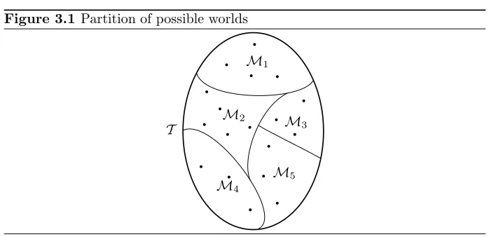
A truth-finding frame incorporates both the available information about re-ality, and the objective of the learning task. The available information about reality is represented by a set of options, the possible worlds, and a conditional distribution that specifies how each possible world works. The objective of the learning task is given by the partition, which divides the possible worlds into

models, clusters of similar worlds. The set of models M can be regarded as a

discretisation of the set of possible worldsT. Figure 3.1 depicts a typical

par-tition of possible worlds into models. We want to obtain as much information as possible about the true model, i.e. the model that contains the true state of nature.

3.1.2 Examples

Throughout this chapter we use three running examples as an illustration. Let

Y ={H,T} be the sample space of outcomes of a coin flip. We denote bypθ

the distribution that assigns probabilityθ to H, and hence 1−θto T. We use

the following three variants of the biased coin scenario:

• Biased Coin (BC). As in the introduction to this thesis, we use modelsthe

(35)

[image:35.595.97.446.119.288.2]

Chapter 3. Truth finding 3.1. Formalisation

Figure 3.1 Partition of possible worlds

M1

M2 _M

3

M4

M5

T

• Reduced Biased Coin (RBC). In this simplified version, we replace the

second model of BC bythe coin favours heads considerably.

• Binary Biased Coin. (BBC). In this even more simplified version, we use

two singleton models: the coin mildly favours tails and the coin favours

heads a lot.

The models for each of the variants are formally specified in Table 3.1. In each

case, we have models M = {M1,M2}, possible worldsT = SM, and

truth-finding frame

F=T,Y,M,hpθiθ∈T

.

3.1.3 Truth-finding problem

Now we can formally state the worst-case truth-finding problem. Let F be a

frame. The unknown actual worldθ∗ _{∈ T} _{must be classified according to}_M_,

based on data generated from pθ∗. Ideally, we would like to identify the true

modelM∗_:=_M₍_θ∗_{), but in our probabilistic framework we cannot do this with}

certainty. Instead we use the data to construct a probability distributionm on

models, wherem(M) represents our degree of belief thatM∗₌_M_.

An outsider knowing M∗ _{can evaluate}_m _{by computing the log loss, which}

is given by L(M∗_,_m_{), where}

L(M,m) :=−logm(M).

Recall that this is the amount of information that we, usingm, lack about the

true model. Namely, it is the number of bits that the outsider has to transmit

Table 3.1Biased coin example models

M1 M2

BC 1/2 1/2,1

RBC 1/2 (0.6,1]

[image:35.595.97.441.652.722.2]

(36)

3.2. Truth-finding game Chapter 3. Truth finding

to us to allow us to identifyM∗ _{with certainty. For convenience, we define}

L(θ,m) := L(M(θ),m).

We do not know M∗_{, so we cannot evaluate the performance of} _m_{. This}

impasse can be overcome by considering strategies. A strategyf is a function

that assigns a distribution on models toeach outcome, i.e. a conditional

distri-bution on models given outcomes. A strategyf can be pitted against a possible

worldθ, yielding the following expected loss, orrisk

R(θ, f) := E

Y∼pθ

h

L θ, f(Y)i. (3.1)

Hence the problem becomes this: find a strategyf that minimises the

worst-case risk, i.e. attains

V = inf

f sup_θ_∈TR(θ, f).

We will show in§3.4.2 that there is always anf that attains V.

3.1.4 Assumptions

We must assume that |M| ≥2 for there to be a truth-finding problem, and we

must assume|Y| ≥2 for there to be a basis for a solution. To simplify analysis,

we make the following additional assumptions.

Assumption 3.2. The set of outcomesY is finite.

Assumption 3.3. The set of models Mis finite.

These assumptions, albeit restricting, capture many practically interesting cases, for instance the biased coin example. In the anvil drop example, the outcomes are time measurements. The set of time measurements is in prin-ciple uncountable, but it is naturally discretised by contemporary stopwatch manufacturers, who supply a fixed number of decimal digits.

These assumptions allow us to identify distributions onYandMwith points

in the unit|Y|- and|M|-simplices. Recall from Definition 2.6 that the unit n

-simplex is given by

∆n:=

n

p∈Rn₊ |pT1= 1o.

This identification allows us to regard each model M ∈Mas a subset of ∆|Y|.

We do not have to place any restrictions on the set of possible worlds, nor on

the mechanics.1 _{We see this as a passed sanity check; these are the two places}

where the complexity of real-world applications will be reflected.

3.2 Truth-finding game

Worst-case expected-value optimisation problems like the truth-finding prob-lem are naturally thought of as two-player games with chance moves, and this viewpoint proves fruitful in our case. The players in the truth-finding game are

1_{Of course, there are the standard measurability conditions. We list all the conditions in}

MoL 2007 02: Discovering the truth by conducting experiments

Discovering the truth by conducting

experiments

MSc Thesis

(

Afstudeerscriptie

)

MSc in Logic

Prolusion

Contents

List of Figures

List of Tables

List of Protocols

Chapter 1

Introduction

1.1

Problem statement

1.2

Basic terminology

1.3

Selection tasks

1.4

Experiments

1.5

Contribution of the thesis

Related work

Organisation of the thesis

Acknowledgements

Chapter 2

Preliminaries

2.1

General notation

2.2

Set theory

℘

℘

2.3

Linear algebra

2.4

Convex analysis

2.5

Probability theory

℘

2.6

Information theory

2.6.1

Quantifying information

2.6.2

Basic coding

2.6.3

Advanced coding

2.7

Game theory

Chapter 3

Truth finding

3.1

Formalisation

Notational conventions

3.1.1

Truth-finding frames

3.1.2

Examples

3.1.3

Truth-finding problem

3.1.4

Assumptions

3.2

Truth-finding game