MNRAS487,4751–4767 (2019) doi:10.1093/mnras/stz1438 Advance Access publication 2019 May 24
Through thick or thin: multiple components of the magneto-ionic medium
towards the nearby H II region Sharpless 2–27 revealed by Faraday
tomography
Alec J. M. Thomson ,
1‹T. L. Landecker,
2John M. Dickey,
3N. M. McClure-Griffiths,
1M. Wolleben,
4E. Carretti ,
5A. Fletcher,
6Christoph Federrath,
1A. S. Hill ,
2,7,8S. A. Mao ,
9B. M. Gaensler ,
10,11M. Haverkorn,
12S. E. Clark,
13†
C. L. Van Eck
10and J. L. West
101Research School of Astronomy and Astrophysics, Australian National University, Canberra, ACT 2611, Australia
2Dominion Radio Astrophysical Observatory, National Research Council Canada, P.O. Box 248, Penticton, BC V2A 6J9, Canada 3School of Natural Sciences, Private Bag 37, University of Tasmania, Hobart, TAS 7001, Australia
4Skaha Remote Sensing Ltd., 3165 Juniper Drive, Naramata, BC V0H 1N0, Canada 5INAF – Istituto di Radioastronomia, Via P. Gobetti 101, I-40129, Bologna, Italy
6School of Mathematics, Statistics and Physics, Newcastle University, Newcastle-upon-Tyne NE13 7RU, UK 7Department of Physics and Astronomy, University of British Columbia, Vancouver, BC V6T 1Z1, Canada 8Space Science Institute, Boulder, CO 80301, USA
9Max-Planck-Institut fur Radioastronomie, D-53121 Bonn, Germany
10Dunlap Institute for Astronomy and Astrophysics, University of Toronto, 50 St. George Street, Toronto, ON M5S 3H4, Canada 11Department of Astronomy and Astrophysics, University of Toronto, Toronto, ON M5S 3H4, Canada
12Department of Astrophysics/IMAPP, Radboud University, P.O. Box 9010, NL-6500 GL Nijmegen, the Netherlands 13Institute for Advanced Study, 1 Einstein Drive, Princeton, NJ 08540, USA
Accepted 2019 May 22. Received 2019 May 21; in original form 2019 February 20
A B S T R A C T
Sharpless 2–27 (Sh2–27) is a nearby HIIregion excited byζOph. We present observations of polarized radio emission from 300 to 480 MHz towards Sh2–27, made with the Parkes 64 m Radio Telescope as part of the Global Magneto-Ionic Medium Survey. These observations have an angular resolution of 1.35◦, and the data are uniquely sensitive to magneto-ionic structure on large angular scales. We demonstrate that background polarized emission towards Sh2–27 is totally depolarized in our observations, allowing us to investigate the foreground. We analyse the results of Faraday tomography, mapping the magnetized interstellar medium along the 165 pc path to Sh2–27. The Faraday dispersion function in this direction has peaks at three Faraday depths. We consider both Faraday thick and thin models for this observation, finding that the thin model is preferred. We further model this as Faraday rotation of diffuse synchrotron emission in the Local Bubble and in two foreground neutral clouds. The Local Bubble extends for 80 pc in this direction, and we find a Faraday depth of−0.8±0.4 rad m−2. This indicates
a field directed away from the Sun with a strength of−2.5±1.2μG. The near and far neutral clouds are each about 30 pc thick, and we find Faraday depths of −6.6±0.6 rad m−2 and
+13.7±0.8 rad m−2, respectively. We estimate that the line-of-sight magnetic strengths in the
near and far cloud areB,near≈ −15μG andB,far≈ +30μG. Our results demonstrate that
Faraday tomography can be used to investigate the magneto-ionic properties of foreground features in front of nearby HIIregions.
Key words: polarization – HIIregions – ISM: magnetic fields.
E-mail:[email protected] †Hubble Fellow
1 I N T R O D U C T I O N
Magnetic fields are crucial dynamical drivers in the Galactic inter-stellar medium (ISM). They are responsible for injecting significant
energy into the ISM (Heiles & Haverkorn2012; Beck & Wielebinski
2019 The Author(s)
2013; Beck2016). Magnetic fields play roles in star formation and
turbulent gas flows (Padoan & Nordlund2011; Federrath & Klessen
2012; Federrath2015), and also have profound consequences for
the initial mass function of stars (Federrath et al.2014; Offner et al.
2014). Despite their importance, much remains unknown regarding
both the magnitude and structure of these magnetic fields. This has arisen from the general difficulty in measuring the strength and structure of magnetic fields in the ISM.
Radio spectro-polarimetry is one of the most effective ways to
study interstellar magnetic fields (Han2017). Linearly polarized
emission is produced within the Milky Way by relativistic electrons emitting synchrotron radiation as they orbit around magnetic fields. At radio frequencies, this emission suffers Faraday rotation as it propagates towards the observer through the magneto-ionic medium (MIM). Thus, observations of Galactic polarized radio emission contain a wealth of information on the Milky Way’s magneto-ionic structure.
Faraday rotation causes the polarization angle (χ) of an
electro-magnetic wave to rotate from an initial angle (χ0) at wavelength
λ:
χ(λ2)=χ0+λ2φ, (1)
whereφis the Faraday depth (Burn1966; Brentjens & de Bruyn
2005):
φ(d)≡0.812 0
d
ne(r)B(r)dr
rad m−2, (2)
andneis the thermal electron density in cm−3,B is the
line-of-sight (LOS) component of the magnetic field inμG, anddris the
incremental distance along the LOS in pc to a source at distanced.
In the case of a single rotating region in front of a polarized source, referred to as a ‘Faraday screen’, the Faraday depth is equivalent to the rotation measure (RM):
RM≡ dχ
d(λ2)
rad m−2. (3)
We follow the definitions of Brentjens & de Bruyn (2005)
through-out, we quantify Faraday rotation using Faraday depth, and we refer to RMs from extragalactic sources. Due to the strong wavelength de-pendence, low-frequency radio observations of polarized emission are very sensitive for measuring Faraday rotation in the magneto-ionic medium (MIM). The determination of the Faraday depth from Galactic synchrotron emission is non-trivial, however, due both to the complexity of the Galactic MIM and the mixing of emission and Faraday rotation in the same volume. This can be overcome by mapping polarization across many frequency channels in a technique called ‘Faraday tomography’. We outline this technique in Section 2.
The large angular scales of diffuse Galactic polarized emission calls for global radio spectro-polarimetric survey. The Global
Magneto-Ionic Medium Survey (GMIMS, Wolleben et al.2009)
was devised specifically to probe the MIM of the Milky Way. This survey will ultimately measure diffuse polarized emission across the entire sky from 300 MHz to 1.8 GHz using single-dish telescopes, giving excellent sensitivity to a wide range of Faraday structures. Results from the GMIMS high-band North
(GMIMS-HBN, Wolleben et al.2010a), taken with the DRAO 26 m telescope,
have been used directly to investigate the magneto-ionic properties
of a nearby HIshell (Wolleben et al.2010b), the North Polar Spur
(Sun et al.2015), and the Fan Region (Hill et al.2017), and they
are incorporated into other work analysing all-sky emission (e.g.
Zheng et al.2017; Dickey et al.2019).
The nearby HII region Sharpless 2–27 (Sh2–27) appears in
various radio polarization observations. Sh2–27 surrounds the star
ζOph which is located at [l, b] ∼ [6.3◦,+23.6◦] (van Leeuwen
2007). The region subtends about 10◦ on the sky and is readily
identifiable in Hαimages. HIIregions are highly ionized regions
of the ISM, and thus have a greater thermal electron density over
the typical Galactic warm neutral medium (Ferri`ere (2001)). In
the presence of magnetic fields, HIIregions have a strong effect
on observations of radio polarization (e.g. Gaensler et al.2001).
At 2.3 GHz in the S-band Polarization All Sky Survey (S-PASS,
Carretti et al.2019) Sh2–27 has been identified as a Faraday screen,
modulating the polarization angle but not producing polarized
emission itself (Iacobelli et al.2014; Robitaille et al.2017,2018).
In polarization observations at 1.4 GHz, such as GMIMS-HBN, Sh2–27 can be identified as a depolarizing region. Wolleben et al. (2010b) used the depolarization of Sh2–27 to constrain the distance
of polarized emission through a nearby HIshell. The magneto-ionic
properties of Sh2–27 were directly investigated by Harvey-Smith,
Madsen & Gaensler (2011) using the NVSS catalogue of
point-source RMs (Taylor, Stil & Sunstrum2009). This region stands out
in the Taylor et al. (2009) catalogue, and derivative maps such as
Oppermann et al. (2012, 2015), due to high values of RM from
extragalactic sources seen through it.
In this paper, we present results from the low-band Southern Global Magneto-Ionic Medium Survey (GMIMS-LBS) towards Sh2–27. Using these data, we are able to isolate a column of fore-ground MIM for analysis with Faraday tomography. The distance
to Sh2–27 is known to be∼180 pc (Gaia Collaboration et al.2016,
2018), which means we are able to map results from polarization
ob-servations within that distance. We provide additional background and definitions we use that are specific to radio polarimetry in Section 2. We describe the GMIMS-LBS observations in Section 3, including the application of Faraday tomography. In Section 4, we present the results of these observations towards Sh2–27 and show that it is depolarizing the background emission in the GMIMS-LBS band. We conclude that Sh2–27 is acting as a ‘depolarization wall’ for extended structures, and can therefore be used to constrain distances in Faraday tomography. We describe the structure in the GMIMS-LBS Faraday depth cubes towards Sh2–27 in Section 4.2. We analyse how this structure maps to distance along the LOS in Section 5. In Section 5.1, we consider a Faraday thin interpretation in combination with data on the local ISM to both reconstruct the magnetic field structure and estimate the magnetic strength along the LOS. In Section 5.2, we consider an alternate model using Faraday thick structures. We discuss our results in Section 6, and provide a summary and conclusion in Section 7.
2 B AC K G R O U N D
2.1 Faraday tomography
It is highly unlikely that any given LOS in the Galaxy would be as simple as a Faraday screen. With this in mind, the technique of
Faraday tomography (also known as RM synthesis) (Burn1966;
Brentjens & de Bruyn2005; Heald, Braun & Edmonds2009) was
developed. This method applies a discrete Fourier transform to the
complex polarization as a function ofλ2. The primary result of this
technique is the Faraday dispersion function (F(φ)), the polarized
flux as a function of Faraday depth. This function is spectral in nature, and we refer to it as the Faraday spectrum. The output parameters of Faraday tomography are set by the behaviour of the ‘RM spread function’ (RMSF). The effective resolution of the
Faraday tomography towards Sh2–27
4753
Faraday spectra (δφ) is given by the width of the RMSF at full-width
at half maximum (FWHM) (Brentjens & de Bruyn2005):
δφ≈ 2
√ 3
λ2, (4)
where λ2=λ2
max−λ 2
min is the bandwidth inλ
2-space, andλ2
max
andλ2
minare the maximum and minimum observedλ2, respectively.
The largest observable value of Faraday depth (φmax) is set by the
width of the observedλ2channels (δλ2):
φmax≈
√ 3
δλ2 (5)
Finally, the smallest observedλ2sets the maximum scale observable
in Faraday depth space:
φmax-scale≈ π λ2 min
. (6)
Sources that produce a broad feature in the Faraday spectrum are referred to as ‘Faraday thick’. Specifically, a source is ‘thick’ if
λ2 φ 1, where φis the extent of the source inF(φ) observed
atλ2(Brentjens & de Bruyn2005). Such features can be modelled
as a mixture of a coherent and turbulent magnetic field that produces both synchrotron emission and Faraday rotation of background
polarized emission (Burn1966; Sokoloff et al.1998). Conversely,
a feature is Faraday thin ifλ2 φ1. Faraday thin features can be
modelled as aδfunction in the Faraday spectrum.
Observational restrictions on wavelength coverage have a strong effect on Faraday tomography. These effects can be mitigated using deconvolution techniques. Currently, the most popular algorithm is RM-CLEAN(Heald et al.2009), which replaces the ‘dirty’ RMSF with a smooth Gaussian restoring beam. This reduces the effect of sidelobes that are present in the ‘dirty’ Faraday spectra.
2.2 Depolarization
Depolarization is a common feature of almost all radio polarization observations, with the exception of polarized emissions from pul-sars. This effect can occur through three primary mechanisms (Burn
1966; Tribble 1991; Sokoloff et al. 1998): depth, beam, and
bandwidth depolarization. Depth depolarization refers to the effect
of Faraday thick sources inλ2space. Such sources lose polarized
flux as a function ofλ2. Beam and bandwidth depolarization arise
from observational parameters. In the former case, the variation of Faraday depth occurs spatially within the beam of the telescope. Bandwidth depolarization occurs when significant Faraday rotation occurs within one frequency channel.
In low-frequency observations depolarization features become far more common and are often associated with ionized regions of
the ISM, such as HIIregions. As these features depolarize emission
from behind them, they can be used as distance indicators in radio polarization observations.
Despite their higher Faraday resolution, low-frequency
observa-tions can face an issue by not observing polarized flux at shortλ2.
The result of missing this emission is that sources with a Faraday
thickness greater thanφmax-scaleare ‘resolved out’, whereby broad
features are lost leaving only narrow features present in Faraday depth space. In practice, this can give rise to an ambiguity between a Faraday thick feature or a number of Faraday thin features.
A ‘depolarization wall’ (Hill2018) is a form of spatially discrete
depolarization. Whilst conceptually similar to the ‘polarization
horizon’ (Uyaniker et al.2003), a depolarization wall arises when a
[image:3.595.309.548.102.267.2]specific and discrete depolarizing object (such as an HIIregion)
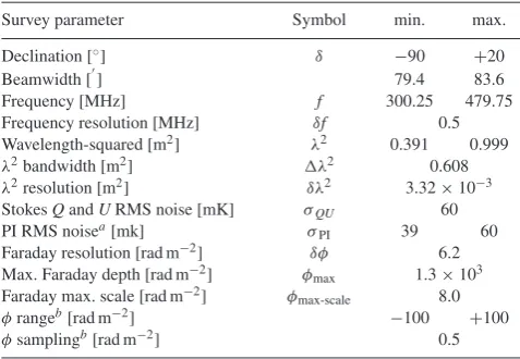
Table 1. Summary of the observational parameters of the GMIMS-LBS (Wolleben et al.2019, Dickey et al.2019).a– This range is determined by
the high and low signal-to-noise limits.b– We select these values during
Faraday tomography.
Survey parameter Symbol min. max.
Declination [◦] δ −90 +20
Beamwidth [] 79.4 83.6
Frequency [MHz] f 300.25 479.75
Frequency resolution [MHz] δf 0.5
Wavelength-squared [m2] λ2 0.391 0.999
λ2bandwidth [m2] λ2 0.608
λ2resolution [m2] δλ2 3.32×10⁻³
StokesQandURMS noise [mK] σQU 60
PI RMS noisea[mk] σPI 39 60
Faraday resolution [rad m−2] δφ 6.2 Max. Faraday depth [rad m−2] φmax 1.3×103
Faraday max. scale [rad m−2] φmax-scale 8.0
φrangeb[rad m−2] −100 +100
φsamplingb[rad m−2] 0.5
lies along the LOS. When an LOS passes through a wall, the background polarized emission is totally depolarized. Whether or not an object acts as a wall in a given observation will depend on
both the observedλ2and the angular resolution. Polarization walls
have a great utility for analysing results of Faraday tomography. Despite the large amount of information contained within Faraday spectra, mapping that structure to physical space is challenging. If the distance to a depolarization wall can be determined, however, that places a constraint on the distance along which the observed
Faraday structure occurs. This is highly analogous to the use of HII
regions as free–free absorbers of Galactic synchrotron emission
(e.g. Nord et al.2006; Su et al.2018).
3 O B S E RVAT I O N S
3.1 GMIMS low-band south
Recently, we completed GMIMS-LBS with the Parkes 64 m tele-scope. A complete description of these observations is provided
in Wolleben et al. (2019). These observations measure diffuse
polarized emission (StokesI,Q, andU) across the entire Southern
sky from 300 MHz to 480 MHz with a spectral resolution of 0.5 MHz.
Here, we analyse the Faraday spectral cubes from this survey.
These spectra have been deconvolved using RM-CLEAN (Heald
et al.2009). We summarize the properties of these data, including
the parameters resulting from Faraday tomography, in Table1. The
long wavelengths and high spectral resolution result in a unique
property for this survey: a very fine Faraday resolution of δφ=
6.2 rad m−2, smaller than the Faraday max-scale of the survey. This
is the first large-scale sky survey withφmax-scale> δφat frequencies
above 250 MHz. This property means that onlyfeatures that are
broader thanφmax-scale will be resolved out. Without this property,
the observed spectra become more complex (Dickey et al. 2019)
and their interpretation more difficult.
It is also important to consider the behaviour of noise in Faraday
spectra. The RMS noise in the StokesQandUspectra isσQU =
60 mK. We primarily consider the absolute value of the Faraday dispersion function, which represents the polarized intensity. When
analysing the polarized intensity, the variance (σPI) is given by a
Rayleigh distribution (Wardle & Sramek1974; Heald et al.2009):
σPI=
4−π
2 σQU ≈0.66σQU, (7)
in the low signal-to-noise limit. For increasing signal-to-noise, the
variance approaches a Gaussian distribution andσPI=σQU.
3.2 Complementary data
We use a number of other data sets to complement our GMIMS-LBS
observation. Finkbeiner (2003) combines data from the Virginia
Tech Spectral Line Survey (VTSS, Dennison, Simonetti & Topasna
1998), the Southern H-Alpha Sky Survey (SHASSA, Gaustad et al.
2001) and the Wisconsin H-alpha mapper (WHAM, Haffner et al.
2003) to produce an all-sky Hαintensity image with a resolution
of 6. We use these data to identify Sh2–27 and other HIIregions
around it.
The Taylor et al. (2009) catalogue provides measurements of
RM towards extragalactic point sources as measured by the Very Large Array (VLA). These data are derived from NRAO VLA
Sky Survey (NVSS, Condon et al. 1998), and provide a source
density of∼1 deg−2. Since these data were taken at L-band, and
with 45resolution, they are far less susceptible to depolarization
effects. We are therefore able to investigate the Faraday rotation through Sh2–27 with these data.
The STructuring by Inversion the Local Interstellar Medium
project1(STILISM, Lallement et al.2014, 2018; Capitanio et al.
2017) provides information on the three-dimensional structure of
the nearby ISM. These data are produced using dust reddening of
starlight (e.g. Vergely et al. 2010; Lallement et al.2014; Green
2014; Capitanio et al.2017; Green et al.2018), with stellar parallax
distances fromGaia, to map dust features in the nearby ISM. We
use the data cube from this project, which covers a 4 kpc by 4 kpc by 600 pc grid around the Sun.
4 R E S U LT S
4.1 Depolarization from Sh2–27
Polarized intensity is very low in GMIMS-LBS towards Sh2–27.
The depolarizing effect of Sh2–27 in our data can be seen in Fig.1,
which shows the peak polarized intensity from theCLEANFaraday
spectra in the region towards Sh2–27. We also show the combined
SHASSA and WHAM Hα intensity from Finkbeiner (2003) as
white contours. We identify two important features from this map. First, while the area towards Sh2–27 is clearly reduced in polarized intensity with respect to the surrounding emission, the polarized intensity is well above the noise (60 mK). Second, a strong but narrow depolarization feature extends out to the right from the edge of the Sh2–27’s depolarization region. We will address these features in turn with respect to several depolarization mechanisms. GMIMS-LBS is able to probe magneto-ionic effects in great detail due to the long wavelengths observed. Consequently, these observations are also more sensitive to depolarization features.
A Faraday depth of about ±940 rad m−2 would be required to
completely depolarize our lowest frequency observation through bandwidth depolarization. Such extreme values are rarely observed away from the Galactic plane. We therefore do not expect bandwidth depolarization to affect our observations.
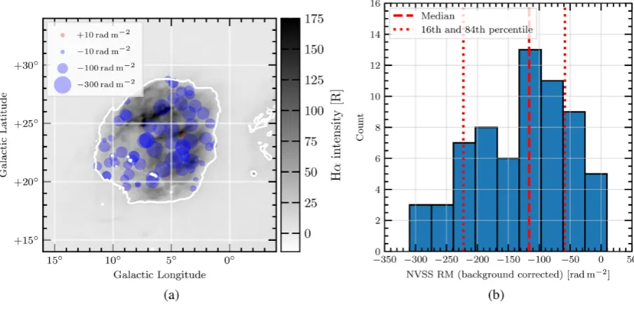
[image:4.595.309.544.54.222.2]1https://stilism.obspm.fr/, version 4.1, accessed October 2018
Figure 1. The peak PI in the Faraday cube towards Sh2–27. Contours are Hαintensity from Finkbeiner (2003) at 30 R. We label the five visible HII regions, and their corresponding central stars (white stars), in this region as: (a) – Sh2–27 /ζOph, (b) – Sh2–7 /δSco, (c) – Sh2-1 /πSco, (d) – Sh2–9 /σSco, (e) – RCW 129 /τSco. We show the beam as a white circle in the lower-left corner. We note that in Hαthere are four other nearby HII regions that appear close on the sky to Sh2–27. In contrast to Sh2–27, these HIIregions have no discernible effect on the polarization data. We identify a depolarization wall that occurs approximately within the Hαcontour of Sh2–27. We further find that the depolarized feature extending horizontally across this map is a depolarization canal.
Table 2. Faraday rotation properties for various ISM phases. Col.(1): The ISM phases. Col.(2): The local electron density of the ISM (Ferri`ere2001; Heiles & Haverkorn2012). Col.(3): The Faraday rotation per unit distance, assuming a 2μG LOS magnetic field with no reversals. Col.(4) and (5): The depth along the LOS after which depth depolarization will filter out polarized emission for LOFAR and GMIMS, respectively.
Phase ne Faraday rotation Path length
[cm−3] [rad m−2pc−1] [pc]
LOFAR GMIMS-LBS
CNM 0.016 0.026 42 310
WNM 0.0007 0.0011 1000 7300
WIM 0.25 0.41 2.7 20
WPIM 0.1 0.16 6.9 50
HIM 0.0034 0.006 200 1400
Given the large beam of GMIMS-LBS (81 arcmin at 300 MHz), beam depolarization is likely to be a significant effect. We quantify the beam depolarization towards Sh2–27 using point-source RMs. These values probe Faraday rotation along the entire LOS out to the edge of the Galaxy, thus allowing the investigation of the intervening ISM.
Here, we apply a similar analysis to Harvey-Smith et al. (2011),
but instead we will obtain the variation in Faraday depth across Sh2–27, and thus estimate the beam depolarization in GMIMS-LBS
using the Taylor et al. (2009) catalogue. We adopt the same boundary
conditions and background RM correction as Harvey-Smith et al.
(2011), given in their Table 2. This results in 65
background-corrected RMs through Sh2–27, which we show in Fig.2(a). We
also show the distribution of these RMs in Fig.2(b). From these
RMs, we find a median value of −166 rad m−2 and a standard
deviation ofσRM=78 rad m−2. To analyse howσRMchanges across
angular scales, we compute the second-order structure function
(SFRM) of the RMs on Sh2–27, as defined by Haverkorn, Katgert &
[image:4.595.309.546.428.519.2]Faraday tomography towards Sh2–27
4755
Figure 2. The Taylor et al. (2009) RMs towards Sh2–27. Here, we apply the selection criteria and background correction of Harvey-Smith et al. (2011). (a) The spatial distribution of RMs on Sh2–27. (b) The histogram of the RM distribution towards Sh2–27. We also show the median RM (dashed line), and 16th and 84th percentiles (dotted lines). We use these data to demonstrate that Sh2–27 is a depolarization wall to the diffuse emission measured by GMIMS-LBS. The high RM values shown here are not detected in our Faraday spectra as polarized emission from behind the HIIregion is totally depolarized.
de Bruyn (2004):
SFRM( θ)= [RM(θ)−RM(θ+ θ)]2, (8)
where θ is the angular distance on the sky between two LOS,
and . . . represents the average on all pairs of separation θ.
We estimate the errors in the structure function by utilizing Monte Carlo error propagation. Assuming that the errors in the Taylor
et al. (2009) RMs are Gaussian-distributed, we take 1 000 samples
of a Gaussian distribution for each RM on Sh2–27 and propagate
the entire distribution through the SFRMcomputation. We find that
the function remains flat from the angular scale of Sh2–27 (∼10◦)
to scales smaller than the beamwidth of our observations. We can therefore expect that the variation in RM as computed across the entire Sh2–27 region will be about the same as the variation within the GMIMS-LBS beam.
We estimate that the variance in Faraday depth due to Sh2–27 can be related to the variation in RM by:
σ2 RM=σ
2 HII+σ
2 gal+σ
2 exgal+σ
2
err (9)
where σHII is the variation in Faraday depth caused by
turbu-lent structures in the HII region, σgal≈8/sin (b)≈20 rad m−2
(Schnitzeler 2010) is the variation along the rest of the LOS
through the Galaxy, σexgal≈6 rad m−2 (Schnitzeler2010) is the
variation in RM due to contribution from the intrinsic Faraday
rotation of the extragalactic source, andσerr= 10.1±0.4 is the
measurement error in RM. In this way we estimate the variation in
Faraday depth of Sh2–27 to beσHII≈74±1 rad m−2. The degree
of beam depolarization can be quantified by either the Burn (1966)
depolarization law, or by the Tribble (1991) depolarization law if
the depolarization (compared to the intrinsic polarization fraction)
is<0.5:
DPBurn =e−2σ
2λ4
(10)
DPTribble= 2√2√1N σ λ2, (11)
where DP is the depolarization fraction (the ratio of observed to
intrinsic PI),σ is the variation in Faraday depth,λis the observed
wavelength, andNis the number of independent, randomly varying
areas within the beam. Across our band, the Burn depolarization
factor is <exp (−1700) and the Tribble depolarization factor is
<1/(130√N) (<0.008 forN= 1). In either case, the emission
behind Sh2–27 is strongly beam depolarized in our survey. We find, however, a significant polarized signal towards Sh2–27. Since an
HIIregion does not produce polarized emission itself, we are able to
proceed treating Sh2–27 as a ‘depolarization wall’ and we conclude that the polarized emission that we observe must arise between the Sun and Sh2–27.
Hill (2018) does note, however, that it is possible for polarization
to make its way through a depolarizing volume, such as an
HII region, using a semi-analytic mock observation matched to
GMIMS-LBS. Their model included a lower-density HII region
than Sh2–27. We ran a version of their model with a density and magnetic field which matches estimates for Sh2–27 (Harvey-Smith
et al. 2011). Some polarized radiation does leak through at the
Faraday depth of the HIIregion in the model, but the polarized
intensity is10 per cent of the background polarized intensity. In
the model, there are components of the Faraday spectrum at Faraday depths comparable to what would be observed for background sources; we do not see components at the Faraday depths seen
by Harvey-Smith et al. (2011), so the depolarization may be more
wall-like than in the Hill (2018) model.
We identify the large depolarized feature that extends to the right from Sh2–27 as a depolarization canal. Depolarization canals are a common feature of many polarization maps. These canals can occur from a variety of physical scenarios, but most commonly
occur through one of two mechanisms (Fletcher & Shukurov2006;
Fletcher & Shukurov2007): either a strong gradient or discontinuity
in Faraday depth across the sky, or depth depolarization along the LOS. Both of these mechanisms can produce depolarization which
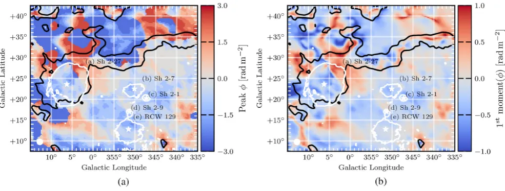
is the width of the telescope beam. In Fig.3(a), we show an image of
the Faraday depth at the peak PI in the range−3< φ <+3 rad m−2.
Figure 3. (a): The Faraday depth at the peak PI in the region of Sh2–27 in the range−3< φ <+3 rad m−2. (b): The first moment of the Faraday spectrum
computed in the range−3< φ <+3 rad m−2. White contours are Hαintensity from Finkbeiner (2003) at 30 R. Black contours are of the peak PI (for allφ)
at 0.3 K RMSF−1. We label the five visible HIIregions, and their corresponding central stars (white stars), as in Fig.1. We show the beam as a white circle in
the lower-left corner. The range−3< φ <+3 rad m−2is used to select only the peak around 0 rad m−2.
We select this restricted range in order to find the peak around
0 rad m−2. The Faraday depth structure towards Sh2–27 is different
to that along the feature. On Sh2–27, the peakφis relatively smooth
and constant (φ <0). In contrast, there is a clear discontinuity in
φalong the canal, as well as a gradient towards Galactic North.
We confirm that these discontinuities are not artefacts of two peaks of similar heights by inspecting the first moment of the Faraday
spectra in Fig.3(b). This map shows the same discontinuities and
gradients as the peakφ map, which indicates that these are true
features of the Faraday depth structure. Areas with a discontinuity
in φ show depolarization on the order of a beamwidth, which
leads us to the conclusion that the feature is a depolarization canal. We note that the canal is slightly wider than the beamwidth, but this is explained by a combination of a discontinuity and a
gradient inφ. Both of these effects generate depolarization canals,
and both appear in close proximity in the peak φ map. The
depolarizing effects then blend into a wider canal. We conclude that this feature is distinct from Sh2–27 and we do not discuss it further.
4.2 Faraday spectra towards Sh2–27
We find a consistent structure in the Faraday spectrum towards
Sh2–27, shown in Fig.4. In the left-hand panel of Fig.4, we show
azimuthal averages (through a full rotation) of the Faraday spectrum
in polarized intensity as a function of radius on the sky fromζOph.
For the region towards Sh2–27, we find a triple-peak structure,
which is absent in the regions away from the HIIregion. In the
middle panel of Fig.4, we can see that each peak is well above
our noise threshold and well fit by a singleCLEANcomponent. For
comparison, we show the RMSF for the same region. It is clear that the triple-peak structure is not generated by sidelobes in the RMSF. The polarized intensity also increases significantly away from Sh2–27, correlating with the loss of the triple-peak structure. As the foreground structure is unlikely to correlate precisely with the boundary of Sh2–27, we conclude that the foreground structure we probe towards Sh2–27 is overwhelmed by higher intensity back-ground emission in directions away from the depolarization wall.
To identify the Faraday depth of the peaks on Sh2–27, we
first apply the peak-finding algorithm from Duarte (2015) to find
the Faraday-resolution-limited peaks in the azimuthally averaged spectra. We only search for peaks above our noise threshold of 60 mK. From this, we find the triple-peak structure extends radially
for 5.5◦fromζOph, which is almost exactly the radius of Sh2–27
in Hα. We fit three Gaussians to the triple-peak region excluding
structures below our noise threshold and obtain the means of the three peaks weighted by the inverse variance from the radial
profile, (1) −7.4±0.4 rad m−2, (2)−0.8±0.4 rad m−2, and (3)
+6.2±0.4 rad m−2.
5 A N A LY S I S
When multiple peaks are present in a low-frequency Faraday spec-trum, two primary interpretations are possible: either the features are of separate origin, or the peaks arise from a Faraday-thick medium which has been resolved out. We follow the method of Van Eck
et al. (2017) (hereafterCVE17) for separating these scenarios. We
estimate the distance to the front of Sh2–27 using the distance
toζOph. We use the parallax distance to this star from theGaia
DR2 survey (Gaia Collaboration et al.2016,2018), specifically the
error-corrected distance estimates provided by Bailer-Jones (2015),
182+−5333pc. Taking the region to be a sphere-centred onζOph with
an angular radius of 5.5◦on the sky, we find the distance to the front
of the region is 164+−4830pc.
5.1 Faraday thin models towards Sh2–27
In this section, we present a Faraday-thin model of the foreground ISM towards Sh2–27, and show that it can accurately reproduce
the observed StokesQandUspectra as a function ofλ2. We also
consult additional data which can give information on the structure of the foreground column of ISM.
In general, the complex polarization of a Faraday-thin component is given by:
P(λ2)=exp2i(χ0+φ0λ2, (12)
Faraday tomography towards Sh2–27
4757
Figure 4. The Faraday depth structure towards Sh2–27. Left-hand panel: Azimuthal averages of the Faraday spectrum as a function of radius fromζOph. Middle panel: MedianCLEANand dirty Faraday spectrum, andCLEANcomponents, on the Sh2–27 region (as defined by Harvey-Smith et al. (2011)). We also label the first, second, and third primary peaks. Right-hand panel: Median dirty andCLEANRMSF on the Sh2–27 region.
whereχ0is the initial polarization angle of the emission andφ0is
the Faraday depth of the component. We obtain the de-rotatedχ0
for peaks 1, 2, and 3 using:
χ0=χ1−φ0λ20 mod 180◦, (13)
where χ1 is the polarization angle at the peak in the Faraday
spectrum, and λ2
0 is the de-rotated wavelength-squared as per
Brentjens & de Bruyn (2005). We construct model spectra as the
sum of three Faraday thin components using the Faraday depth of each peak, their corresponding initial angles, and amplitudes
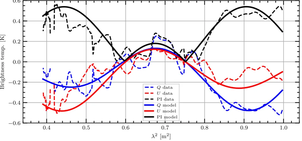
of 0.18 K. We show both the average Stokes Q, U, and PI λ
spectrum on Sh2–27 and the Faraday-thin model in Fig. 5. We
have not used any fitting routine, rather we have simply constructed the model from the average values we infer from the Faraday spectrum.
There are two factors to consider as we construct a physical model of MIM along the LOS. We must consider where the polarized
Figure 5. Faraday-thin model spectra towards Sh2–27. Dashed lines: Average StokesQ,U, and PIλ2spectra towards Sh-27 from GMIMS-LBS. Solid lines:
Faraday-thin model derived from the average Faraday spectrum.
[image:7.595.49.550.468.702.2]emission arises and determine to what degree the Faraday rotation occurs. We make this consideration under the constraint of the
∼160 pc path to the front of Sh2–27. Meaning that we are analysing
small, localised structures, with a size scale much less than a kiloparsec. We will first consider the sources of Faraday rotation before considering the source of polarized emission. A Faraday-thin model does not necessarily exclude mixed emission and rotation, but for a model to be considered Faraday thin in our context the Faraday
thickness should not exceed theφmax-scaleof our observations.
The most likely contributors in the ISM to Faraday rotation of low-frequency polarized emission are the cold and warm neutral medium (CNM and WNM), the warm ionized medium (WIM), and the hot ionized medium (HIM). There are no large molecular clouds towards Sh2–27, as indicated by the absence of obscuration of the
Hαemission from the HII region. We can consider the amount
of Faraday rotation each ISM phase is likely to contribute along the LOS, and quantify the path-length at which each phase will be resolved out of our observations. Here, we take local electron
densities of the various ISM phases from Ferri`ere (2001) and Heiles
& Haverkorn (2012), and we assume a typical regular magnetic field
value of 2μG (Sun et al.2007) with no reversals.CVE17conducted
a similar analysis in the LOFAR band, finding that only emissions produced in the WNM would not be resolved out. We summarize
these results in Table2, comparing the survey characteristics from
GMIMS-LBS and LOFAR. Since the φmax-scale of GMIMS-LBS
is nearly eight times that of LOFAR, our survey is much less susceptible to resolving out Faraday-thick structures. We therefore
cannot construct a similar model toCVE17, where interpretation of
the polarized emission was tied to the absence of depolarization in the WNM. Instead, the features that we observe must be explained by enhancements in the MIM along the LOS.
The different ISM phases along the LOS will each contribute differently to the Faraday rotation of synchrotron emission, due to their different magneto-ionic properties. The Local Bubble consists
of a hot ionized medium (HIM), atne=0.005 cm−3 (Cordes &
Lazio 2002; Shelton 2009), filling a volume around the Sun.
Synchrotron emissions produced inside the Local Bubble should
create a peak in the Faraday spectrum around 0 rad m−2, as emission
produced close to the Sun should experience minimal Faraday
rotation. Our peak 2 is consistent with 0 rad m−2at 2σ. We therefore
interpret peak 2 as emission that is produced within the Local
Bubble. At 1σ of confidence, we observe−0.8±0.4rad m−2of
Faraday rotation through this volume.
Faraday rotation in the Local Bubble also affects the features
which arise behind it; that is, we must subtract the−0.8 rad m−2
contribution from peaks 1 and 3. Applying this moves peaks 1 and 3
to−6.6±0.6 rad m−2and+7.1±0.6 rad m−2, respectively. We can
constrain what is producing these features by analysing how LOS components of the ISM are contributing to Faraday rotation. Taking
our values from Table2, assuming these phases are contributing
∼7 rad m−2of Faraday rotation would require a path-length of about
270 pc, 6 kpc, 17 pc, 40 pc, and 1.2 kpc respectively.
Because of the short path-length (164+48
−30pc) to the front of Sh2–
27, the only possible candidates are the CNM, WIM, WPIM. Neutral
gas is typically traced using HIobservations. We inspect the HI
emission in the region of Sh2–27 from HI4PI (Ben Bekhti et al.
2016). Due to the proximity of Sh2–27 to the Sun, HIemissions
produced in this region crowd around 0 km/s, making kinematic
distances unreliable. We do find indications of HIself-absorption,
however, in the HIspectra towards the HIIregion, which indicates
the presence of cold atomic gas. We are therefore motivated to look
to the STILISM project (Lallement et al.2014; Capitanio et al.
2017; Lallement et al.2018), which traces the CNM and provides
the LOS distances to these neutral structures.
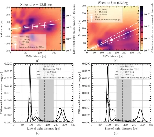
We show a series of slices through the STILISM cube in Fig.6.
The Local Bubble appears as a void surrounding the Sun in these data. We find that the distance to edge of the Local Bubble is 80 pc in
the direction of Sh2–27. Taking an electron density of 0.005 cm−3,
we derive a magnetic field strength of−2.5±1.2μG in the Local
Bubble, aligned away from the Sun.
The location of Sh2–27 correlates with a region of relatively
lower dust content in STILISM, as expected around an HIIregion,
compared to neutral clouds. Between the front of Sh2–27 and the edge of the Local Bubble, two dust features appear. These
regions occur at ∼95 pc and∼135 pc and are each∼30 pc deep
along the LOS. The distance error from the reddening inversion
in this area is ∼11 pc. We provide the spatial coverage of these
clouds in the contours of Fig. 7(a). The near cloud covers the
entire region towards Sh2–27, whilst the far cloud only covers the lower-left portion of the region. Comparing the Faraday spectra between these areas, we find that the triple-peak structure changes to a double-peak in the upper-right portion of the region, as shown
in Fig.7(b). We see that there is neutral material in front of Sh2–
27, and its location correlates with the Faraday spectra, so we can explain the Faraday properties of the foreground column without any WIM or WPIM along the line of sight. The magnetic fields
need to be more intense, however, than the ∼2μG we assumed
previously.
In higher density regions of the ISM, magnetic fields become
compressed (Crutcher et al.2010) and highly ordered, even in a
relatively neutral medium (Clark, Peek & Putman2014; Kalberla
et al.2017; Gazol & Villagran2018; Tritsis, Federrath & Pavlidou
2019). The dust features towards Sh2–27 are composed of CNM,
and thus are a higher density region of neutral ISM. We can estimate
the density in these clouds using a dust-to-gas ratio. Liszt (2014)
find a ratio of HI column density (N(HI)) to dust reddening
magnitude (E(B − V)) of N(HI)=8.3×1021cm−2E(B−V)
for for|b|>20◦andE(B−V)0.1 mag. This corresponds to
a number density (n(HI)) to differential colour excess ratio of
∼2700 cm−3/(mag pc−1). For the two foreground clouds, we find
a total number density ofntot∼50 cm−3and∼12 cm−3, which is
consistent with typical values in the CNM (Ferri`ere2001). Increased
electron density and magnetic fields in the dust features are evidently providing increased Faraday rotation over the more tenuous inter-cloud medium.
The observed triple-peaked Faraday spectrum can be reproduced from a simple model of the magneto-ionic structure towards Sh2–
27. We summarize this model of the MIM towards Sh2–27 in Fig.8.
In this model, we first assume a constant synchrotron emissivity (ε)
along the entire LOS towards Sh2–27. We interpret peaks 1 and 3 to be associated with the dust features. Such peaks would be produced if both clouds have stronger Faraday rotation, with LOS magnetic fields of opposite directions and with the cloud further from the Sun having stronger LOS magnetic field than the closer one. This must be the case to produce two peaks. If the clouds had similar strength LOS magnetic fields, emission produced behind both clouds would
be Faraday rotated by the closer cloud to∼0 rad m−2. Further, we
are able to associate peak 3 with the far cloud from the change in the Faraday spectrum on and off the cloud. This means that peak 1
arises from the near cloud. To summarize, assuming a uniformε,
the triple-peak structure can be created from the far cloud with a
Faraday depth of+13.7±0.8 rad m−2, the near cloud with Faraday
depth of−6.6±0.6 rad m−2, and a peak near 0 rad m−2from the
Local Bubble. Emission produced in the warm inter-cloud regions
Faraday tomography towards Sh2–27
4759
Figure 6. Three-dimensional dust structure towards Sh2–27 from STILISM (Lallement et al.2014; Capitanio et al.2017; Lallement et al.2018). In all panels, the solid line shows the LOS through the position ofζOph, and the dashed lines are LOS through the outer bounds of the HIIregions. (a) Slice through data cube at a constant latitude. (b) Slice through data cube at a constant longitude. (c) and (d) show the LOS profiles for panels (a) and (b), respectively. is not depolarized, but undergoes an increased amount of Faraday
rotation in the neutral dust clouds.
We confirm the viability of the model by constructing a simple 1D numerical simulation of the Faraday rotation produced by this
model. Into this model, we input LOS values forB,ne, and
pseudo-ε, scaling the total emission to 1 flux unit. From this, we obtain
StokesQand Uin the GMIMS-LBS band and perform Faraday
tomography. We show the resulting Faraday spectra in Fig.9. In
this evaluation of the simulation, we takeB in the near and far
cloud to be−15μG and+30μG, respectively, with the rest of
the LOS having 2μG. We find that the resulting Faraday spectrum
is relatively insensitive to the sign of the intra-cloud and Local
Bubble field directions. When we assume a uniformε we obtain
a triple-peak spectrum which is dominated by the component near
0 rad m−2, as shown in Fig.9(a). This is likely because this is
over-estimating the contribution of emission from the Local Bubble. More realistically, the magnetic fields in the HIM of the Local
Bubble are likely to be weak (Hill et al.2012,2018), and therefore
theεin this region should be reduced relative to the rest of the LOS.
In Fig.9(b), we show the result of setting theεof the Local Bubble
to be 10 per cent of the remainingε. This produces three peaks of
approximately equal height in the Faraday spectrum. It is possible that this same structure may arise from a more complicated LOS composition. In the absence of data to motivate such a model, this simulation demonstrates that our observed Faraday structure can be produced from a simple model.
We can also determine how tenable this model is by calculating the polarization fraction. To do this, we must also estimate the total synchrotron intensity towards Sh2–27. As Sh2–27 is a depolariza-tion wall, we need to only consider the synchrotron emission from in
front of the region. Roger et al. (1999) measured the total intensity
towards a number of HII regions, including Sh2–27, at 22 MHz
and estimated the synchrotron emissivity. They findε=159 K/pc
at 22 MHz, but they note that the emissivity towards Sh2–27 was
Figure 7. (a): The first moment map of the Faraday spectrum (as in Fig.3b). White contours are Hαintensity from Finkbeiner (2003) at 30 R. Black, dashed contours show STILISM dust reddening at 90 pc, corresponding to the near neutral cloud. Black, solid contours show STILISM dust reddening at 135 pc, corresponding to the far neutral cloud. Green circles show the positions for the Faraday spectra in the right-hand panel. (b): Faraday spectra for two lines-of-sight towards Sh2–27. The upper panel shows an LOS which intersects with only the near cloud. The lower panel shows an LOS which intersects both neutral clouds.
very high relative to other HIIregions, and that Sh2–27 might be
not completely optically thick at 22 MHz. We investigate whether
this is the case using values from the literature. The opacity (τ) of
an HIIregion at a particular frequency (ν) is given by Mezger &
Henderson (1967):
τ=3.28×10⁻⁷
Te
104
−1.3 ν [GHz]
−2.1
EM, (14)
wherene≈2 cm−3(Wood et al.2005), EM=240±26 cm−6pc
(Celnik & Weiland 1988) is the emission measure, and Te is
the electron temperature. TakingTe=7000 K givesτ = 0.38 at
22 MHz, meaning Sh2–27 is not optically thick. Using this opacity,
we re-derive a foreground emissivity ofε=37+−2315. More recently,
Su et al. (2018) calculated the synchrotron emissivity towards
many HII regions at 76.2 MHz using the Murchison Widefield
Array (MWA). They find an average value of 1±0.5 K pc−1 at
76.2 MHz. Taking a spectral index ofβ= −2.5 (whereI∝νβ), the
emissivity at the GMIMS-LBS mid-band frequency of 390 MHz
is ε=0.017±0.008 K pc−1. This value is also consistent with
our recomputed value from Roger et al. (1999) assuming the
same spectral index. Using the scaled emissivity from Su et al.
(2018), we estimate the total flux arising in front of Sh2–27 is
2.8+2.5
−1.6K.
The use of depolarization walls is conceptually similar to using
free–free absorption of StokesIby HIIregions. Similarly, we can
determine the total received polarized emission towards Sh2–27. Using our Gaussian fit for the three Faraday thin components, we integrate the polarized intensity over the range of Faraday depths to determine the total polarized flux. From this, we find a total
polarized flux of∼0.4 K. Taking our previous estimate of the total
intensity, this results in a polarization fraction of 12+−166 per cent.
Given that spatial variation in Faraday depth will cause significant beam depolarization, this fraction is relatively high. This value further supports our finding that the magnetic fields causing the
Figure 8. A cartoon of the magnetic field structure we observe along the LOS towards Sh2–27. We indicate the approximate distance to each feature along the bottom of the figure. We shade the two neutral clouds grey, indicating their increased density over other LOS components. The hatched region corresponds to the front of Sh2–27, behind which we receive no polarized emission. We give the values for the Faraday depths in each region. Arrows indicate the magnetic field direction in the Local Bubble and the two neutral clouds, as determined from our observations.
[image:10.595.51.541.538.684.2]Faraday tomography towards Sh2–27
4761
Figure 9. Simulated Faraday spectra of our Faraday-thin model. The LOS distribution of the MIM is identical for each model, with only the emissivity changing. (a) Uniform emissivity along the entire LOS. (b) Emissivity in the Local Bubble reduced by 90 per cent.
observed Faraday rotation towards Sh2–27 have a highly ordered component.
Finally, we estimate the magnetic field strengths in the neutral clouds. We have determined that the far cloud has a Faraday
depth of∼ +14 rad m−2and the near cloud a Faraday depth of
∼ −7 rad m−2. From equation (2), we also need to estimaten
e, and
the path-length through each region (L). We find no pulsars between
the Sun and Sh2–27 in ATNF Pulsar Catalogue (Manchester et al.
2005),2 and since Sh2–27 is the dominant Hα emission source
in this direction it is not possible to constrain thene from these
observations. As such, we present the LOS magnetic field strength
as a function of the total number density (ntot), the ionization fraction
(Xe), andL. We also estimate the strengths taking reasonable values
from Ferri`ere (2001) and our estimates above:
B,near≈ −15μG ntot
20 cm−3
Xe
1×10⁻³
L 30 pc
B,far ≈ +30μG ntot
20 cm−3
Xe
1×10⁻³
L 30 pc
5.2 Faraday thick models towards Sh2–27
We can also decide whether the Faraday structure towards Sh2–
27 is Faraday thick using theCVE17 polarization flux method.
After performing Faraday tomography, the PI spectra have units of K/RMSF. To obtain polarized flux, we must convert these
units to K/(rad m−2). This conversion factor of rad m−2/RMSF
is given by the integrated area (A) under the CLEAN Gaussian
RMSF. For the region towards Sh2–27 in GMIMS-LBS this
factor is 7.3 rad m−2/RMSF. Note, that for LOFAR observations,
CVE17 obtained a conversion factor of near unity, whereas
2Catalogue version: 1.59, Accessed 26thof November 2018.
the factor for GMIMS-LBS is nearly an order of magnitude higher.
We can now model the depolarization of a Faraday-thick medium
in GMIMS-LBS. We model this as a ‘Burn slab’ (Burn1966), the
simplest Faraday thick model. In Faraday depth space a Burn slab is a tophat function, which corresponds to the following complex
polarization inλ2:
Pλ2=exp2iχ0+φ0λ2sin
φλ2
λ2 , (15)
where φ0 is the central Faraday depth of the slab, and φ is
the width, or Faraday thickness, of the slab, andχ0again is the
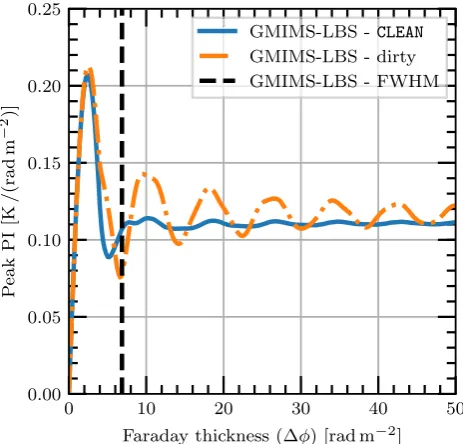
initial polarization angle. This model has the additional advantage of resolving out the least as a function of Faraday thickness; that is, other Faraday-thick models will be filtered out more strongly. We model observations using GMIMS-LBS by evaluating this complex
polarization using λ2 values observed by GMIMS-LBS, taking
the height of the slab to be 1 K, and then performing Faraday tomography on the resulting spectra. As the model is resolved out, the ‘observed’ Faraday spectrum is split into two peaks which also reduce in magnitude. We show this reduction as a function of
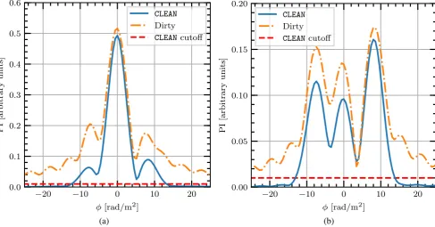
Faraday thickness (matching fig. A.1. of Van Eck et al. 2017) in
Fig.10. We note that this function is smooth compared toCVE17
because we have also appliedRM-CLEANto our synthetic spectra
(not doing so results in an oscillation due to interference between the sidelobes of the depolarized peaks). We find that if the Faraday thickness of the slab is greater than the FWHM of the RMSF, then the depolarization factor is about 11per cent. For a Faraday thickness less than that, the depolarization factor varies signifi-cantly, reaching a peak depolarization factor of about 21per cent at
2.4 rad m−2.
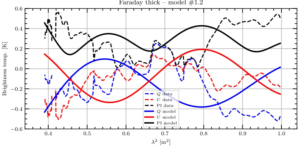
There are three possible thick models that could apply to our observations (1): either peaks 1 and 2 are edges of a thick slab, (2): peaks 2 and 3 are edges of a slab, or (3): peaks 1 and 3 are the
Figure 10. The depth depolarization of a Burn slab as a function of Faraday thickness, as observed by GMIMS-LBS. The peak PI is taken from a synthetic Faraday tomography observation of a Burn slab with a height 1 K and a variable thickness. Blue, dash–dotted: Depolarization from dirty spectra. Orange, solid: Depolarization from CLEAN spectra. Black, dashed: The FWHM of the RMSF.
edges of the slab. In each case the third peak would be provided by a Faraday thin component. We will only consider cases (1) and (2), as case (3) will result in greater missing flux. In both cases, we cannot know which peak represents the leading edge of a slab
a priori. This condition, however, only sets the direction of the coherent magnetic field along the LOS, and does not affect the degree of missing flux. The Faraday thicknesses for models (1)
and (2) are 6.6±0.6 rad m−2and 7.1±0.6 rad m−2, respectively.
The heights of peaks 1, 2, and 3 are 0.185 ± 0.002 K/RMSF,
0.190±0.005 K/RMSF, and 0.168±0.006 K/RMSF, respectively.
For simplicity, we can consider both of these cases together
as a slab of thickness ∼7 rad m−2, and a depolarized peak of
∼0.18K/RMSF. Taking the conversion factor of 7.3 rad m−2/RMSF
gives the height of the depolarized peak as∼0.024 K/(rad m−2). A
Faraday thickness of∼7 rad m−2will correspond to a depolarization
factor of∼11per cent, and therefore the height of the slab will be
∼0.23 K/(rad m−2). Integrating across the slab results in a polarized
flux of∼1.6 K. From our estimate above, a Faraday thin component
would provide about 0.1 K of flux.
For the ε we calculate above, the polarization fraction would
therefore be 62+−8129per cent. For comparison, the maximum
theoretical polarization fraction for synchrotron emission is 75
per cent (Rybicki & Lightman1986), but this will only occur when
the magnetic field generating the synchrotron emission is perfectly uniform. Such high values are highly unlikely to arise in the diffuse ISM.
We also evaluate theλ2spectra for each Burn slab model in a
similar manner to the Faraday thin case. We show the resulting
spectra in Section A (FigsA1–A6).None of these models recreate
the average spectra well, especially in comparison to the thin model. From both this finding, and our analysis of the polarized flux from a Burn slab model, we conclude that a Faraday-thick model is unlikely to apply here.
6 D I S C U S S I O N
Faraday tomography is a powerful method for probing the MIM of the Galactic ISM. Faraday depth, however, can vary in a non-monotonic fashion along the LOS and mapping structure in the Faraday dispersion function is therefore difficult. The use of depolarization to constrain distances to polarized features has been applied in many diffuse polarization surveys (e.g. Wolleben et al.
2010b; Hill et al.2017). We have shown that at low frequencies this analysis can be extended. If a depolarization feature can be identified as a depolarization wall, then any observed polarized emission can be constrained to the region along the LOS in front of the feature. In GMIMS-LBS, we are sensitive to large angular scales, but our large beam also constrains us to this type of analysis only on large depolarization regions. Additionally, the current
spatial density of extragalactic RMs (e.g. Taylor et al. 2009) is
∼1 RM/deg2, which also restricts the analysis of beam
depolar-ization Future polarized surveys, such as POSSUM (Gaensler et al.
2010) from the Australian SKA Pathfinder (ASKAP), aim to deliver
∼100 RM/deg2. With such data, the type of analysis we present here
can be extended to higher angular resolution with observations from
aperture synthesis telescopes. Furthermore, distances to HIIregions
are being well constrained by the HIIRegion Discovery Surveys
(HRDS, SHRDS Bania et al.2010; Brown et al.2017).
Understanding of the density–magnetic field relationship in the ISM is of great importance to many processes. Recent observations
(e.g. Wolleben et al. 2010b; Clark et al. 2014; Kalberla et al.
2017; Tritsis et al.2019) and numerical simulations (e.g. Gazol &
Villagran2018) have shown that even in the diffuse ISM magnetic
fields can be compressed and ordered. Our observations are highly compatible with this picture, and our model of the ISM towards Sh2– 27 shows that magnetic fields have become ordered and magnified
in nearby dust clouds. Crutcher et al. (2010) show that in densities
associated with the CNM, magnetic fields are measured be on the
order of 5μG, but can be as high as 10–20μG. Wolleben et al.
(2010b) use Faraday tomography to measure the magnetic field
in large, nearby HIshell. They determine an LOS field strength
of 20–34μG. Clark et al. (2014) estimate a total magnetic field
strength in the Riegel–Crutcher HIcloud of 10–50μG, using a
Chandrasekhar–Fermi-like method. McClureGriffiths et al. (2006)
previously constrained that the total magnetic field in the
Riegel-Crutcher cloud should be at least 30μG. Tritsis et al. (2019) analyse
a similar region in Ursa Major, finding a total magnetic field strength
of 10–20μG. Our magnetic field estimates are broadly consistent
with these measurements. We note however, that each of these cases
represents an atypical cloud, as compared with Crutcher et al. (2010)
results for the same density. Further investigation of the clouds we find towards Sh2–27 is required to understand whether such a special case, such as compression within a shell wall, occurs here.
7 S U M M A RY A N D C O N C L U S I O N
In this paper, we have made use of the highly sensitive GMIMS-LBS observations to probe the magneto-ionic structure of the nearby
ISM. We achieve this by identifying the nearby HIIregion Sh2–27
as a depolarization wall. The magneto-ionic properties of Sh2– 27, as revealed by extragalactic RMs, prevent polarized emissions produced behind the region at 300–480 MHz from propagating through it. We are then able to perform Faraday tomography on the observed polarized emission knowing that the structure we observe must originate between the Sun and the front of Sh2–27, a path length of only 160 pc.
Faraday tomography towards Sh2–27
4763
We find a consistent triple-peaked structure in the Faraday spectrum in the region towards Sh2–27. We conclude that the structure is highly unlikely to arise from a resolved out Faraday thick source, but rather should be caused by magneto-ionic enhancements along the LOS. We draw this conclusion from both consideration of the polarized flux and by modelling Faraday thick and thin spectra. We find that only the thin model reproduces the observations well. Using 3D ISM maps we identify two neutral features in front of Sh2–27 as well as the ionized region of the Local Bubble. The Local Bubble extends for 80 pc in the direction of Sh2–27, and the two clouds lie in the remaining space in front of Sh2– 27 and are each about 30 pc thick. Given the constraint on the LOS structure we also find that the observed Faraday structure cannot arise from a tenuous ionised region. Rather, the structure must arise from magneto-ionic enhancements. We are able to associate the three peaks in our Faraday spectrum with the two neutral clouds and the Local Bubble. We confirm the viability of this model using both a simple 1D simulation, and an analysis of the polarized flux. Following this, we find a Faraday depth in the
local bubble of−0.8±0.4rad m−2, meaning that magnetic field
is aligned away from the Sun in this direction. Assuming that this Faraday rotation occurs uniformly throughout the Local Bubble, this Faraday depth corresponds to a LOS magnetic field strength of
−2.5±1.2μG. In the near and far clouds we obtain Faraday depths
−6.6±0.6 rad m−2and+13.7±0.8 rad m−2, respectively. These
Faraday depths correspond to LOS magnetic fields of opposite alignment in each cloud.
Here, we have considered only a small region in the GMIMS-LBS. We chose this region as the morphological correlation between
the polarization structure and the HIIregion Sh2–27 is immediately
apparent. We have shown that interpretation of features in these data requires careful analysis and combination with extragalactic polarization observations and additional tracers of the ISM. We have shown that GMIMS observations are highly complementary
to newly released survey data such asGaiaand will be of great use
for interpretation of results from the upcoming MWA and ASKAP surveys.
AC K N OW L E D G E M E N T S
The authors wish to thank JinLin Han for his constructive input. AT acknowledges the support of the Australian Government Research Training Program (RTP) Scholarship. N. M. M.-G. ac-knowledges the support of the Australian Research Council through grant FT150100024. C. F. acknowledges funding provided by the Australian Research Council (Discovery Project DP170100603 and Future Fellowship FT180100495), and the Australia-Germany Joint Research Cooperation Scheme (UA-DAAD).
The Parkes Radio Telescope is part of the Australia Telescope National Facility which is funded by the Commonwealth of Aus-tralia for operation as a national facility managed by CSIRO. This work has made use of data from the European Space Agency (ESA)
missionGaia(https://www.cosmos.esa.int/gaia), processed by the
Gaia Data Processing and Analysis Consortium (DPAC, https:
//www.cosmos.esa.int/web/gaia/dpac/consortium). Funding for the DPAC has been provided by national institutions, in particular
the institutions participating in theGaiaMultilateral Agreement.
We further acknowledge high-performance computing resources provided by the Australian National Computational Infrastructure (grant ek9) in the framework of the National Computational Merit Allocation Scheme and the ANU Allocation Scheme. This research
made use of Astropy,3a community-developed core Python package
for Astronomy (Robitaille et al.2013; Price-Whelan et al.2018).
This research made use of APLpy, an open-source plotting package
for Python (Robitaille & Bressert2012). We have made use of the
‘cubehelix’ colour-scheme (Green2011).
R E F E R E N C E S
Bailer-Jones C. A. L., 2015,Publ Astron. Soc. Pacific, 127, 994
Bania T. M., Anderson L. D., Balser D. S., Rood R. T., 2010,ApJ, 718, L106
Beck R., 2016, Astron. Astrophys. Rev., 24, 4
Beck R., Wielebinski R., 2013, Planets, Stars and Stellar Systems, Vol. 68. Springer, Netherlands, Dordrecht, p. 641, preprint (arXiv:1302.5663) Ben Bekhti N. et al., 2016,A&A, 594, A116
Brentjens M. A., de Bruyn A. G., 2005,A&A, 441, 1217 Brown C. et al., 2017,AJ, 154, 23
Burn B. J., 1966,MNRAS, 133, 67
Capitanio L., Lallement R., Vergely J. L., Elyajouri M., Monreal-Ibero A., 2017,A&A, 606, A65
Carretti E. et al., 2019, preprint (arXiv:1903.09420) Celnik W. E., Weiland H., 1988, A&A, 192, 316
Clark S. E., Peek J. E. G., Putman M. E., 2014,ApJ, 789, 82
Condon J. J., Cotton W. D., Greisen E. W., Yin Q. F., Perley R. A., Taylor G. B., Broderick J. J., 1998,AJ, 115, 1693
Cordes J. M., Lazio T. J. W., 2002,
Crutcher R. M., Wandelt B., Heiles C., Falgarone E., Troland T. H., 2010,
ApJ, 725, 466
Dennison B., Simonetti J. H., Topasna G. A., 1998,Publ. Astron. Soc. Aust., 15, 147
Dickey J. M. et al., 2019,ApJ, 871, 106
Duarte M., 2015, Notes on Scientific Computing for Biomechanics and Motor Control,https://github.com/demotu/BMC
Federrath C., 2015,MNRAS, 450, 4035 Federrath C., Klessen R. S., 2012,ApJ, 761, 156
Federrath C., Schr¨on M., Banerjee R., Klessen R. S., 2014,ApJ, 790, 128
Ferri`ere K. M., 2001,Rev. Mod. Phys., 73, 1031 Finkbeiner D. P., 2003,ApJS, 146, 407
Fletcher A., Shukurov A., 2006,MNRAS, 371, L21 Fletcher A., Shukurov A., 2007, EAS Publ. Ser., 23, 109
Gaensler B. M., Dickey J. M., McClure-Griffiths N. M., Green A. J., Wieringa M. H., Haynes R. F., 2001,ApJ, 549, 959
Gaensler B. M., Landecker T. L., Taylor A. R., POSSUM Collaboration, 2010, American Astronomical Society Meeting Abstracts #215. p. 470.13
Gaia Collaboration et al., 2016,A&A, 595, A1 Gaia Collaboration et al., 2018,A&A, 616, A1
Gaustad J. E., McCullough P. R., Rosing W., Van Buren D., 2001,Publ. Astron. Soc. Pacific, 113, 1326
Gazol A., Villagran M. A., 2018,MNRAS, 478, 146 Green D. A., 2011, Bull. Astr. Soc. India, 39, 289 Green D. A., 2014, Bull. Astr. Soc. India, 42, 47 Green G. M. et al., 2018,MNRAS, 478, 651
Haffner L. M., Reynolds R. J., Tufte S. L., Madsen G. J., Jaehnig K. P., Percival J. W., 2003,ApJS, 149, 405
Han J. L., 2017,ARA&A, 55, 111
Harvey-Smith L., Madsen G. J., Gaensler B. M., 2011,ApJ, 736, 83 Haverkorn M., Katgert P., de Bruyn A. G., 2004,A&A, 427, 549 Heald G., Braun R., Edmonds R., 2009,A&A, 503, 409 Heiles C., Haverkorn M., 2012,Space Sci. Rev., 166, 293 Hill A., 2018,Galaxies, 6, 129
Hill A. S., Joung M. R., Mac Low M.-M., Benjamin R. A., Haffner L. M., Klingenberg C., Waagan K., 2012,ApJ, 750, 104
3http://www.astropy.org