RIT Scholar Works
Theses Thesis/Dissertation Collections
8-1-2010
Medical image segmentation using
GPU-accelerated variational level set methods
Nathan Prosser
Follow this and additional works at:http://scholarworks.rit.edu/theses
This Thesis is brought to you for free and open access by the Thesis/Dissertation Collections at RIT Scholar Works. It has been accepted for inclusion in Theses by an authorized administrator of RIT Scholar Works. For more information, please [email protected].
Recommended Citation
GPU-Accelerated Variational Level Set
Methods
by
Nathan T. Prosser
A Thesis Submitted in Partial Fulfillment of the Requirements for the Degree of Master of Science
in Computer Engineering
Supervised by
Professor and Departmentent Head Dr. Andreas Savakis Department of Computer Engineering
Kate Gleason College of Engineering Rochester Institute of Technology
Rochester, New York August 2010
Approved by:
Dr. Andreas Savakis, Professor and Departmentent Head Thesis Advisor, Department of Computer Engineering
Dr. Roy Melton, Lecturer
Committee Member, Department of Computer Engineering
Dr. Jay S. Schildkraut,
Rochester Institute of Technology Kate Gleason College of Engineering
Title:
Medical Image Segmentation using GPU-Accelerated Variational Level Set Methods
I, Nathan T. Prosser, hereby grant permission to the Wallace Memorial Library to
re-produce my thesis in whole or part.
Nathan T. Prosser
Dedication
This thesis is dedicated to my father, who always encouraged me to push myself and to try
new things, and to my mother, whose encouragement and kind words helped me get
Acknowledgments
I am grateful for Dr. Andreas Savakis, who gently pushed and guided me along the path
toward actually completing my thesis; for Dr. Jay Schildkraut, who helped me to
understand the algorithm I was working with; for Rick Tolleson, who is always willing to
help with equipment trouble; for my committee, who on short notice read my proposal and
agreed to help; for my wife, who is always right beside me, and never unwilling to
proofread and throw in suggestions; and finally for my God, who loves me enough to put
Abstract
Medical Image Segmentation using
GPU-Accelerated Variational Level Set Methods
Nathan T. Prosser
Supervising Professor: Dr. Andreas Savakis
Medical imaging techniques such as CT, MRI and x-ray imaging are a crucial component of
modern diagnostics and treatment. As a result, many automated methods involving digital
image processing have been developed for the medical field. Image segmentation is the
process of finding the boundaries of one or more objects or regions of interest in an image.
This thesis focuses on accelerating image segmentation for the localization of
cancer-ous lung nodules in two-dimensional radiographs. This process is used during radiation
treatment, to minimize radiation exposure to healthy tissue.
The variational level set method is used to segment out the lung nodules. This method
represents an evolving segmentation boundary as the zero level set of a function on a
two-dimensional grid. The calculus of variations is employed to minimize a set of energy equations
and find the nodule’s boundary. Although this approach is flexible, it comes at significant
computational cost, and is not able to run in real time on a general purpose workstation.
Modern graphics processing units offer a high performance platform for accelerating the
variational level set method, which, in its simplest sense, consists of a large number of parallel
computations over a grid. NVIDIA’s CUDA framework for general purpose computation on
GPUs was used in conjunction with three different NVIDIA GPUs to reduce processing time
Contents
Dedication . . . iii
Acknowledgments . . . iv
Abstract . . . v
1 Introduction . . . 1
2 Image Segmentation . . . 4
2.1 Purpose . . . 4
2.2 Methods . . . 4
2.2.1 Edge-Based . . . 4
2.2.2 Threshold . . . 7
2.2.3 Region Growing . . . 9
2.3 Watershed . . . 10
2.3.1 Active Contours . . . 11
2.4 Level Set Method . . . 13
2.4.1 Velocity-based . . . 13
2.4.2 Energy-based . . . 15
3 Graphics Processing Units . . . 17
3.1 Architecture . . . 19
3.1.1 Processing . . . 19
3.1.2 Memory . . . 22
3.2 Shader Programming . . . 23
3.3 OpenCL . . . 24
3.4 CUDA . . . 25
3.4.1 Programming Model . . . 25
3.4.2 Compute Capability . . . 28
3.4.3 Memory Spaces . . . 28
3.4.4 Limitations . . . 32
3.4.5 Optimization . . . 33
4 Previous Work . . . 36
4.1 Level Set Methods . . . 36
4.2 Level Set Methods for Image Segmentation . . . 37
4.3 GPUs in Medical Imaging . . . 37
4.4 Parallel and GPU Level Set Method Implementations . . . 38
5 The Variational Level Set Method for Lung Nodule Segmentation . . . . 40
5.1 Overview . . . 40
5.2 Energy Terms . . . 42
5.2.1 Contrast Energy . . . 42
5.2.2 Gradient Direction Energy . . . 43
5.2.3 Curvature Energy . . . 43
5.2.4 Prior Energy . . . 43
5.3 Implementation in CUDA . . . 45
5.4 Linear Filtering . . . 46
5.5 Grayscale Morphological Filtering . . . 47
5.6 Gradient and Curvature . . . 47
5.7 LSF Evolution . . . 49
5.8 Energy Summation . . . 50
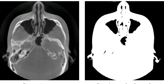
6 Results . . . 51
6.1 Comparisons . . . 55
6.1.1 Multiple Processor Systems . . . 55
6.1.2 Price-to-Performance Ratio Among GPUs . . . 56
6.1.3 Comparison to Other Works . . . 57
7 Future Work and Conclusions. . . 60
7.1 Performance Opportunities . . . 60
7.2 Extension to Three Dimensions . . . 60
7.2.1 Algorithm Development . . . 60
7.2.2 GPU Implementation . . . 62
7.3 Conclusions . . . 63
List of Tables
3.1 Compute Capability . . . 28
5.1 Profiler Results . . . 45
6.1 GeForce GTX 285 Results - Dataset 1 . . . 54
6.2 GeForce GTX 285 Results - Dataset 2 . . . 54
6.3 GeForce GTX 260 Results - Dataset 1 . . . 54
6.4 GeForce GTX 260 Results - Dataset 2 . . . 54
6.5 GeForce 9800 GTX+ Results - Dataset 1 . . . 55
6.6 GeForce 9800 GTX+ Results - Dataset 2 . . . 55
List of Figures
2.1 Sobel Edge Detector . . . 5
2.2 Canny Edge Detector . . . 6
2.3 Bimodal Histogram . . . 7
2.4 Otsu’s Method Thresholding . . . 8
2.5 Watershed segmentation . . . 10
2.6 LSF Evolution . . . 14
2.7 Example of Inverse Gradient . . . 15
3.1 The Rendering Pipeline . . . 18
3.2 NVIDIA’s G80 Architecture . . . 20
3.3 A GT200 Streaming Multiprocessor . . . 20
3.4 CUDA Heterogeneous Processing . . . 26
3.5 CUDA Memory Spaces . . . 29
5.1 Lung Nodule . . . 41
5.2 Binary Tree Reduction . . . 49
6.1 Segmentation Results — Dataset 1 . . . 52
6.2 Segmentation Results — Dataset 2 . . . 52
6.3 Speedup vs. Number of Cores . . . 58
Chapter 1
Introduction
With the proliferation of digital imaging equipment, both in professional and consumer
settings, many applications of image processing have been developed. In the medical domain,
digital imaging is very important, and efficient processing of images can enable applications
that would not otherwise be possible. Image segmentation is an image processing technique
that automatically defines one or more image regions of interest. In medical imaging, this
is often used to generate three-dimensional views of a part of the body for diagnosis or
treatment.
This thesis focuses on the acceleration of a level set segmentation algorithm in order
to minimize radiation exposure to patients undergoing radiation therapy as treatment for
cancerous lung nodules. The treatment procedure consists of two steps: in the first, the
patient’s chest is imaged by a CT scanner, which generates a three dimensional scan of the
chest cavity. These scan data are used to generate a two dimensional “digitally reconstructed
radiograph” that is used at treatment time. Treatment time itself is the second step. The
patient lies on a bed with the radiation source above and an image sensor beneath. The
radiation passing through the patient creates a real-time stream of images through the
sensor. The treatment time images, in conjunction with the digitally reconstructed images,
are used to determine the location of the nodule and focus the radiation beam on it, thereby
Because of the relatively low quality of the images obtained during this procedure, a
robust segmentation algorithm has to be used—a requirement that carries with it heavy
computational demands. In fact, with current general purpose processors, it is impossible
to meet the real time requirement. This thesis primarily focuses on the use of graphics
processing units (GPUs) to accelerate medical image segmentation.
Graphics processors are most often used in video games, three dimensional animation
and CAD programs. They may contain hundreds of simple processing cores, whereas
gen-eral purpose processors typically have only two to four processing units, each of which is
very flexible in what it can do. The massive parallelism that exists in GPUs means that
they can provide much better performance in algorithms that make use of a large number of
independent calculations. It is this property that allows the GPU implementation to achieve
real-time performance when the conventional implementation on a general purpose
process-ing unit could not. GPUs are attractive for computationally-intensive workloads because
they are relatively inexpensive—less than $1000 for high-end devices—and many PCs come
with them pre-installed. Even if this is not the case, add-on boards can be installed easily.
The purpose of this thesis is to implement segmentation using level sets on a GPU, using
NVIDIA’s Compute Unified Device Architecture (CUDA). Three different GPUs at different
price-points are compared: the high-end GeForce GTX 280, the mid-range GeForce GTX
260, and the GeForce 9800 GTX+, a one generation older high-end device. This provides a
rough estimate of the cost-to-performance ratio.
In the remainder of the document, Chapter 2 provides background information on
im-age segmentation in general and on the specific algorithm used here; Chapter 3 describes
used here in detail, including its implementation on the GPU; Chapter 5 reports and
ana-lyzes results; Chapter 6 discusses future work that can be done in this field, including the
Chapter 2
Image Segmentation
2.1
Purpose
A digital image, in its raw form, is essentially an array of numbers that encode brightness
and color. The human visual system is adept at recognizing objects in images, but computers
require complicated algorithms to analyze images in the same way. However, there are many
cases where the accuracy and speed of computer systems is needed. As an example, for a
doctor to outline an organ manually in each slice of a volumetric scan would be tedious and
not a good use of his or her time. Radiation therapy requires the position and size of the
nodule to be known as accurately as possible, and from this information the position and
aperture size of the radiation source is modified.
2.2
Methods
2.2.1 Edge-Based
In cases where the region to be segmented is relatively simple and has strong contrast to its
surroundings, edge-based segmentation methods may be used. Edge detection methods use
the first or second derivative to find image areas where one brightness level or color changes
to another in a small amount of space. Since the derivative computes rate of change of a
function, image regions where pixel values change rapidly have a high spatial derivative.
Input image Sobel gradient image Edge thresholding
Figure 2.1: Sobel Edge Detector
edges.
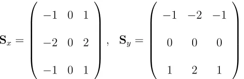
A number of numerical difference schemes can be used to find image edges in this way,
but one of the most widely known is the Sobel edge detector. Although it is not the most
accurate method for finding the derivative, it is simple and works well as an edge detector.
It defines two 3×3 “kernels” that are convolved with the image to find edges. One kernel
approximates a derivative in thex-direction, and the other approximates a derivative in the
y-direction. These kernels are shown below.
Sx=
−1 0 1
−2 0 2
−1 0 1
, Sy =
−1 −2 −1
0 0 0
1 2 1
(2.1)
The results of these two convolution operations are then combined into a gradient
mag-nitude matrix using the following operation:
G=|Gx|+|Gy|. (2.2)
Figure 2.1 is an example of segmentation using a Sobel edge detector and a
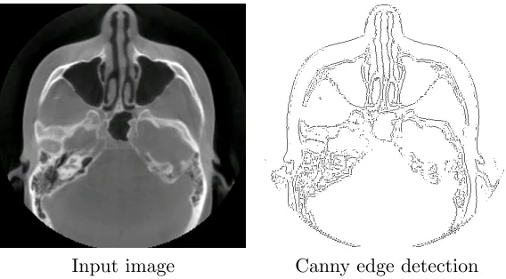
[image:15.612.183.430.478.558.2]Input image Canny edge detection
Figure 2.2: Canny Edge Detector
Segmentation methods that rely on edge detection usually involve an additional step to
find separate edges that should be connected and piece them together to form a complete
boundary. The Canny edge detection method [2] is an example of this approach. The Canny
method first finds the maximum values along each edge so the resulting image has edges
that are a single pixel wide. Two thresholds are then used: one with high value to mask
out any gradient values that are caused by noise or weak edges, and another lower value to
allow many possible edges. A search is conducted along the strongest gradient lines, filling
in areas using the result of the lower mask in places where the edge becomes weak. Figure
2.2 shows edge detection results using the Canny method rather than a simple threshold of
the gradient.
Edge detection methods usually produce good results only in images with high contrast
and clear edges. Since the lung nodule images are noisy and have low contrast, edge detection
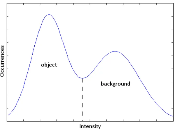
Figure 2.3: A Bimodal Histogram
2.2.2 Threshold
While edge-based segmentation methods attempt to find object boundaries and link them
together to segment the whole object, threshold segmentation operates over the entire image
at once, classifying each pixel as either belonging to the region or not. Threshold methods
attempt in various ways to determine a pixel value or range of values unique to the
segmen-tation target. For example, Figure 2.3 shows a synthetic image intensity histogram where
one object and a background are present, and each has a unique distribution of values. In
this example, the dashed line shows a good threshold value to separate the object from the
background.
Otsu’s method is one way of automatically selecting the proper threshold value. This
method iteratively tries possible thresholds until one is found that maximizes the
inter-class variance. For example, in an 8-bit grayscale image, pixels have integer values in the
Input image Otsu’s method result
Figure 2.4: Otsu’s Method Thresholding
precision, an exhaustive search would not be feasible. The inter-class variance is defined as:
σ2c(t) = ω1(t)ω2(t)·(µ1(t)−µ2(t))2, (2.3)
whereωiare weight factors to account for the probability of a given thresholdtbeing correct,
while µi are the class means [4]. Figure 2.4 shows the result of bi-level thresholding using
Otsu’s method to choose the threshold.
Threshold segmentation can also use varying distance metrics to separate classes. In
some methods, a user selects test points within the segmentation target, and the mean and
standard deviation of these test points are calculated. Then a pixel is classified as part of
the segmentation target if it is within some number of standard deviations from the mean.
This idea can be put to better use in color images, because more data are present. The
Mahalanobis distance metric can be used to model more accurately the range of color values
present in a segmentation target. Given a collection of color samples, each with a red, green
and blue component, a mean vector and covariance matrix are calculated. The Mahalanobis
distance metric is defined as
dM(~x) =
p
whereS is the covariance matrix,~x= (r, g, b)T is the sample under test, and ~µis the mean vector [5]. Then a threshold distance is chosen, often manually, to optimize the segmentation
result.
Although there are ways to account for noise and segmentation targets with gradual
gradients, threshold segmentation algorithms are fundamentally limited by their requirement
for the segmentation target to have a unique and somewhat uniform color or texture. Images
that contain other regions with the same color as the segmentation target, such as the lung
nodule images, will not fare well with threshold segmentation.
2.2.3 Region Growing
Region growing methods start from a set of seed points and recursively examine pixels
touching those seeds to see if they meet some condition suitable to the desired segmentation
result. Any pixels that meet the criteria are added to the seed set, and another iteration
begins with the pixels touching the new seeds. This results in the set of seed points growing
outward from the initial seed or set of seeds.
The criteria for adding to the collection of seed points can be based on basic pixel
inten-sity, some type of similarity to the neighbor pixel, or any other suitable metric. This freedom
can overcome problems like noise and gradual color differences that edge and threshold
seg-mentation cannot deal with, but there is no built-in way to account for shape or occlusion
in region growing methods.
A stopping condition must also be considered. The default condition is when no neighbor
pixels meet the criteria, no new points can be added. Depending on the criteria for addition
and the input image, this may produce a segmentation result larger or smaller than the
Input image Watershed segmentation
Figure 2.5: Watershed segmentation
to the expected number of pixels left to add, if such prior knowledge is available.
2.3
Watershed
Watershed segmentation algorithms are often based in part on edge methods, because the
gradient image is computed first. As its name implies, watershed segmentation divides
images into a number of watershed regions. If the gradient image is projected to three
dimensions, where gradient magnitude is proportional to altitude, a watershed line is defined
as the line on which, if a water drop were placed to one side, it would fall to one local
minimum, while, if the drop were placed on the other side, it would fall to a different local
minimum.
The method as a whole can be visualized using the same three-dimensional gradient map
discussed above. The map is flooded from below, beginning at chosen local minima. As the
water level rises, at some point water from one reservoir will begin to run into another. This
is prevented by building a dam between the two reservoirs that rises with the water level.
Once “land” is no longer visible, the method is complete.
1. Begin with chosen local minima of gradient image
2. Label each chosen minima uniquely
3. Add the neighbors of each minima to a priority queue sorted from low gradient magnitude
to high
4. While the priority queue is not empty, loop:
(a) Remove the first element from the queue
(b) If all of its already-labeled neighbors have the same label, attach the same label
(c) Add all of its unlabeled neighbors to the priority queue
Although this method is more robust with respect to noise and image variation than
the previous methods, it suffers from over-segmentation—that is, too many separate regions
are defined. This effect is shown in the result in Figure 2.5. It can be mitigated by wisely
choosing minima to begin the process, by aggressively smoothing the gradient image, and
by joining regions through other methods. Because the starting point for this method is
still a gradient image, it will not function properly on an input image that does not contain
strong edges. For this reason, it would not perform well for lung nodule segmentation.
2.3.1 Active Contours
Active contour models use a parametric spline to represent an evolving segmentation
bound-ary. The spline is evolved over time in response to minimization of energy functions. These
boundaries are known as “snakes” because of the wriggling movement they exhibit during
The snake is placed near the object boundary by an expert user or by some other
compu-tational method, and then seeks an energy minima. The energy functions used vary based
on the target object, but the “line functional” and the “edge functional” are common terms.
The line functional is based simply on the image intensity,
El=I(x, y), (2.5)
and draws the snake toward dark or light lines in the image.
The edge functional uses the image gradient,
Ee=−|∇I(x, y)|2, (2.6)
which draws the snake toward traditional image edges—contours that have large spatial
gradient values.
When the snake is represented parametrically,vs= (x(s), y(s)), its total energy is defined
as
E =
Z 1
0
Esnake(v(s))ds
= Z 1
0
Eint(v(s)) +Eimage(v(s)) +Econ(v(s))ds. (2.7)
Eimage refers to the energy terms described above. Eint is the snake’s internal energy due
to forces resisting bending, and Econ is the constraint energy.
The snake’s internal energy can be written as
Eint=
1
2 ·α(s)|vs(s)|
2+β(s)|v
ss(s)|2. (2.8)
The coefficient to the first-order term, α, controls the degree to which the snake behaves
which the snake behaves as a rigid plate.
The constraint energy is defined by the user through a collection of “springs” that connect
the snake to a point in the image or another snake. As the spring expands between points
x1 and x2, it exerts an energy of −k(x1−x2)2 on the snake [7].
2.4
Level Set Method
In general terms, a level set of a function is the set of input variables that cause the function
to take on a given constant value: {~x|f(~x) =K}, where ~x is an N-dimensional vector. As
an example, consider a topographic map as a “function” that maps latitude and longitude
to altitude. The constant-altitude curves drawn on these maps are level sets.
Level set methods were first developed as a way to model fluid boundaries, such as a
flame front. They use the zero level set, {~x|f(~x) = 0}, to represent the boundary of the
object being modeled. The symbol φ is usually used to denote the level set function.
Level set movement can be performed explicitly, using forcing functions that depend on
the LSF itself or on the outside environment. Additionally, evolution can be driven without
explicit forcing functions through the use of energy minimization. This is accomplished by
solving differential equations for the change in φ over time.
2.4.1 Velocity-based
The first and most straightforward way to evolve a level set function uses a “velocity”
function to stretch and move the level set function. This function can be a combination of
terms based on both image data and on the level set function itself. Evolution is defined
using the equation below, where V~ is the velocity function:
∂φ ∂t +
~
ϕ(0)
ϕ(t)
x y
y
x
x y
y
x z = ϕ(x, y, t = 0)
[image:24.612.177.431.97.315.2]z = ϕ(x, y, t)
Figure 2.6: LSF Evolution
A commonly used velocity term that is based on the level set function itself is the
cur-vature of the level set function. The equation that defines curcur-vature in level set functions
is:
κ=∇ ·
∇
φ |∇φ|
. (2.10)
In many cases, the level set function’s curvature is used as negative feedback to keep the
level set function smooth, rather than allowing it to develop sharp corners and kinks. This
is done primarily because most physical systems (and objects in images) are curved rather
than sharp and discontinuous. Additionally, sharp corners in the level set translate to high
spatial variability in the level set function, which can overwhelm numerical differentiation
schemes and produce incorrect results. In this case, the velocity functionV~ is normal to the
level set contour with magnitude dependent on curvature [8].
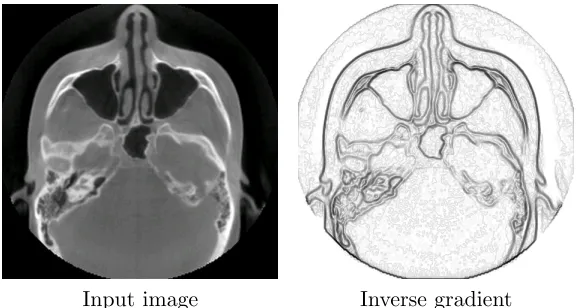
Input image Inverse gradient
Figure 2.7: Example of Inverse Gradient
image processing, a simple way to find image edges is to calculate the spatial gradient of the
image data. Since an edge in an image occurs when color or brightness changes rapidly, edges
have high spatial gradients. Conversely, patches of uniform brightness and color have low
spatial gradients. The inverse gradient, then, allows the level set function to move rapidly
in areas of low spatial gradient (without edges), and to slow dramatically when an edge is
encountered. When the level set function is initialized properly, this will cause the level set
to converge on edges, which has the effect of segmenting the object to which those edges
belong.
2.4.2 Energy-based
Rather than using specific velocity functions to evolve the level set function, an energy
function can be defined based on image and level set data. The energy function is designed
so that its value is minimized at the border of the object to be segmented. Then level set
function evolution is driven by attempts to minimize energy.
In [1], Schildkraut, et al. describe energy functions appropriate to lung nodule
energy terms used take on the form,
E = Z Z
Ω
f(φ, φx, φy, x, y)dxdy, (2.11)
where φ is the level set function, and φx and φy are its partial derivatives with respect to
x and y, respectively. Ω is the variable used to denote the problem domain. For image
segmentation then, Ω refers to the entire image.
To find the energy minimum, the equation above must be minimized with respect to
φ. This requires the use of the calculus of variations, and results in the following partial
differential equation.
∂φ(x, y)
∂t =−
∂f ∂φ−
∂ ∂x
∂f ∂φx
− ∂ ∂y
∂f ∂φy
. (2.12)
The use of energy minimization in conjunction with the level set method is known as
the variational level set method, because of its reliance on the calculus of variations. The
specific energy terms used will be discussed in Chapter 4.
The next chapter first describes the hardware architecture of recent NVIDIA GPUs and
then discusses several programming methods that allow GPUs to perform work other than
Chapter 3
Graphics Processing Units
Graphics processors are devices that are specifically designed for generating images and
sending them to a display device. Early GPUs were only able to composite images and text
into a display buffer, but modern GPUs integrate scene geometry, texture images, lighting
information and special shading programs to deliver a complete three dimensional scene.
Figure 3.1 shows the standard graphics rendering pipeline. To begin, three-dimensional
geometry—usually a collection of triangles—is generated by an application on the host
processor, and handed off to a graphics processor to be rendered. The first stage of the
pipeline operates on triangle vertices, mapping them from three-dimensional scene space to
two-dimensional display space. Since scenes can consist of millions of triangles, and each
mapping operation is completely independent, parallel hardware is important. In this stage,
per-vertex lighting information is computed as well. The second stage is not always used,
and involves mapping an image (called a texture) onto the geometry. In the third stage,
two-dimensional shapes are projected onto the display. Since more than one vertex may be
positioned at a single screen pixel, fragments are generated for each shape and combined to
determine the final pixel color [11].
Early GPUs consisted entirely of fixed function hardware and thus served little purpose
when they were not being used to generate graphics. The only programmability was in what
Generate 3D Geometry
Convert 3D geometry (scene) to 2D geometry (display)
Apply texture (optional)
Rasterize
(convert geometry to pixels)
Composite
(combine fragments into image)
[image:28.612.211.397.76.327.2]GPU
Figure 3.1: The Rendering Pipeline [10]
added to GPUs to enable more inventive and life-like effects. Both the vertex and fragment
processing engines were made programmable to allow dynamic scene transformation and
in-novative lighting techniques. In each new hardware release, the features of the programmable
portion of the hardware were expanded, allowing longer programs, more complex control,
and higher precision. NVIDIA’s G80 hardware was significant on this front, as it used
programmable execution cores as its basis, almost entirely eliminating fixed-function units
[10]. Additionally, it debuted a unified shader architecture: rather than having separate
programmable units for vertex and fragment operations, the same collection of processing
elements could operate on any data. This unified pool of processing resources makes GPUs
3.1
Architecture
NVIDIA’s G80 architecture, along with its successors, G92 and GT200, has almost
com-pletely eliminated hardware specialized to specific stages of the rendering pipeline and
in-stead uses an array of scalar processing elements, as illustrated in 3.2. Put another way,
while older hardware contained special geometry, vertex, and pixel units, G80 has general
purpose cores that can execute geometry, vertex, and pixel programs.
3.1.1 Processing
While traditional processors are designed for low latency and high single-threaded
perfor-mance, GPUs focus on total computational throughput. Given the always limited transistor
budget for microprocessors, GPUs spend many more transistors on computational hardware
rather than on control and management hardware.
Although NVIDIA quotes 240 “CUDA cores” for its GT200 architecture [14], this number
is not as straightforward as it would seem. G80 and later GPUs are divided along three
architectural lines for processing. At the top are thread processing clusters (TPCs), which
comprise 3 streaming multiprocessors (SMs) for GT200 or 2 for G80 and G92. Each SM
consists of 8 scalar processors (SPs); these are what NVIDIA refers to as “CUDA cores” in
marketing material. At each level in the hierarchy some hardware is shared.
TPCs are not discussed in NVIDIA’s literature because they are not visible in the CUDA
programming model. They nevertheless bear mention in an architectural overview. The 2
or 3 SMs in a TPC share a L1 texture cache, which is 16KB in the G80 and G92 or 24KB
in the GT200. They also share the connection to the memory bus associated with the L1
cache.
Figure 3.2: NVIDIA’s G80 Architecture [13]
CUDA device. The number of SMs ranges from 1 in the G80-derived GeForce G100 [15] to
30 in the GT200 flagship device, the GeForce GTX 280 [14].
Each SM consists of a register file (32KB in the G80 and G92 or 64KB in the GT200),
an 8KB cache for constants, 16KB of shared memory and 8 SPs. NVIDIA calls its SM
architecture “SIMT” (single instruction, multiple threads) to differentiate it from the more
common SIMD (single instruction, multiple data) architecture. To a CUDA programmer,
each of the SPs that make up an SM is completely independent, executing its own instruction
stream [16]. Architecturally it is not that simple. Threads are dispatched by the issue logic
in groups of 32 called “warps,” and to achieve maximum performance, each thread in a warp
should take the same branch path. This is not required, however, as it would be in an SIMD
architecture. Since each SP has its own instruction pointer, each thread can take its own
branch path. In the hardware, this is accomplished by first enabling only the threads that
take the first path, then the second, and so on. Because of this, if N different branches are
taken, the performance over that block of code will decrease by a factor of N.
At the bottom layer are the SPs. Although the SPs share the register file, each thread’s
registers are only accessible by itself. Each SP also has its own branch unit, ALU (arithmetic
and logic unit) and FPU (floating point unit). Each SP also has access to 2 FMUL
(float-ing point multiplication)/SFU (special function unit) and 1 64-bit FMAC (float(float-ing point
multiply-accumulate) unit. The SFU is used to calculate complex functions like sine and
cosine, reciprocals and roots. The 64-bit FPU was added to the GT200 architecture to
sup-port double precision floating point math, and is not present in G80 and G92 architectures.
Since the SFUs and 64-bit FPU are shared by the 8 SPs, performance will decrease if they
3.1.2 Memory
NVIDIA’s G80, G92 and GT200 architectures have L1 and L2 cache as in regular
general-purpose processors, but there are several dissimilarities. Data caches for conventional
pro-cessors are fully coherent with main memory and reduce latency on both reads and writes.
Data are cached based on linear spatial locality. In NVIDIA’s GPUs, the caches can be used
only for reads from main memory, and are not coherent. That is, if data are cached, then
changes in main memory will not be propagated to the cache. Additionally, data are cached
based on two-dimensional spatial locality, since textures are basically images.
As was mentioned before, the L1 cache is shared by all elements in a TPC. The L2 cache
is part of the memory controller, and is decoupled from the execution hardware. There are
6 memory controllers in the G80 and G92 and 8 in the GT200; each has 32KB of L2 cache.
Each memory interface is 64 bits wide, which brings the total to 384 bits for the G80 and
G92, and 512 for the GT200.
This 512-bit bus would be largely wasted if the memory controller performed accesses
immediately as they were requested. To avoid this, memory accesses are “coalesced”; that is,
access requests are conglomerated and issued simultaneously. However, in order to coalesce
accesses, certain conditions must be met.
In the G80 and G92, a coalesced access requires that the 384-bit access be aligned on
64-byte boundaries, and confined to a single 64-byte region. Threads must access the data
sequentially—thread 1 must use the first 32 bits, thread 2 must use the second, and so on.
If any of these requirements are not met, each access will be issued individually.
The GT200 relaxes these requirements significantly. The sequential access requirement
not aligned properly, two coalesced accesses will be issued—one for the portion on the first
region, one on the second—rather than splitting them all individually [13].
These caching and coalescing techniques are very important for achieving full memory
throughput, since access latency to the main memory is 400–600 cycles [16]. NVIDIA’s
flagship GT200 device, the GeForce GTX 280, has a memory clock rate of 1107MHz (DDR),
which gives it a peak theoretical bandwidth of 141.7GB/s [14].
3.2
Shader Programming
Before frameworks like CUDA and OpenCL existed, if a GPU were to be used as a general
purpose computation device, programmers had no option but to use the existing graphics
pipeline. As was mentioned previously in this chapter, early programmable GPUs had
sep-arate vertex and fragment processors. However, since more fragments are generated during
rasterization than vertices are input from the application, more computational hardware was
devoted to fragment processing than vertex processing.
Just as in CUDA, the data-parallel portion of the algorithm to be accelerated had to be
turned into a “kernel,” written in a shader language such as the OpenGL Shader Language.
However, rather than determining the range of the output array by specifying grid and
block dimensions, the programmer needed to pass the GPU polygon information to infer
this indirectly. This normally required a single quadrilateral parallel to the display plane
and of the appropriate size. Then the vertex and rasterizer hardware created the millions
of fragments required and invoked the fragment processor on them. Since GPU hardware
allowed a fragment program to write results only to a single coordinate specified by the
position of the input fragment, multiple passes were required if more than a one output per
3.3
OpenCL
OpenCL was proposed by Apple Corporation in June of 2008 to the Khronos Group, a
con-sortium of technology corporations and institutions that oversees such standards as OpenGL
and OpenAL. It was officially released by Khronos in December of 2008. OpenCL is not
restricted to graphics cards; it can target multiprocessor systems, digital signal processors,
or any other high-performance computation device with software support for it.
Like CUDA, OpenCL’s focus is on parallel execution of code, and like CUDA, it uses a
grid abstraction. OpenCL uses grids that consist of “work groups”, which themselves are
grids of “work items”. OpenCL also uses a “context,” which encapsulates information on
the environment in which work units operate: the device type, its memory spaces, and its
work queue.
The various devices in a system that support OpenCL are called “Compute Devices,”
and each of these is composed of one or more “Compute Units.” Each “Compute Unit” is
composed of one or more “Processing Elements.” These are analogous to CUDA’s “device,”
“Streaming Multiprocessor,” and “Scalar Processor,” respectively.
OpenCL’s memory hierarchy is composed of four layers: “Host Memory,” which is the
CPU’s main memory; “Global/Constant Memory,” which resides on the Compute Device
and is accessible to any work groups on it; “Local Memory,” which is shared by the items in
a group; and finally “Private Memory,” which is accessible only to a single work item. As
in CUDA, these memory spaces must be managed manually by the programmer.
The programming language used in OpenCL also shares some traits with CUDA C. It is
based on the C language, with some omissions and enhancements. Some notable omissions
with work items and work groups, the memory spaces mentioned above, and synchronization
between devices.
Since it is possible to target multiple device types with OpenCL code, OpenCL allows
device code to be compiled at run-time by the host, depending on which devices are present
[17].
3.4
CUDA
NVIDIA’s CUDA is a software stack for executing general purpose code on NVIDIA’s
graph-ics processors. It includes a device driver, an API, a compiler and a special variant of the C
language. The compiler supports different output formats—native binary, generic C code,
and PTX assembly—but it is PTX assembly that is most flexible. PTX assembly is a format
that is device-agnostic among NVIDIA devices, which is converted by a just-in-time
com-piler in the driver to native code. The generic C option is useful when debugging, and the
native binary option is useful primarily in situations where a verified, unchanging executable
is needed [16].
3.4.1 Programming Model
At its core, CUDA is a tool to express parallelism in an algorithm, and to execute in
parallel on GPUs. Programs are typically made of sequences that are inherently serial code,
such as reading input data from a disk, and other computational portions that may be
parallelizable. CUDA targets the data parallel, math-intensive portions of the code, using
hundreds of simultaneous threads to speed it up. Because of this dichotomy, code is broken
into “host” sections, written in standard C, C++, or FORTRAN, and “device” sections,
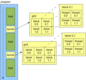
host host host block 0,1 block 1,1 block 0,0 block 1,0 grid kernel kernel thread 0,1 thread 1,1 thread 0,0 thread 1,0 block 0,1 block 0,1 block 1,1 block 0,0 block 1,0 grid thread 0,1 thread 1,1 thread 0,0 thread 1,0 block 0,1 program block 0,0 block 1,0
are called kernels.
Each time a kernel is invoked by host code, the programmer must specify the thread
configuration. This configuration specifies “grid” and “block” dimensions. A grid is a
two-dimensional arrangement of blocks, and a block is a two- or three-two-dimensional arrangement
of threads. Each block can contain up to 256 threads, and is assigned to one and only one
multiprocessor until all of its threads return. This arrangement gives CUDA scalability: if
running on a device with one SM, each block will execute sequentially until all have finished.
However if a more capable device is used, many blocks will be able to execute concurrently.
Figure 3.4 shows how a CUDA program is be separated into host and GPU portions as well
as the way threads are arranged in a grid.
Once the kernel is running on the device, each thread must be able to determine which
portion of the work it should tackle. This is done using the built-in variables threadIdx,
which determines the thread’s position within the block, blockDim, which determines the
number of threads in the block, blockIdx, which determines the block’s position within
the grid, and gridDim, which determines the number of blocks in the grid. Each of these
variables has an x, y, and z member. As an example, consider a grid of data where each
thread is assigned to one element. That thread’sxposition within the grid can be computed
as
x=threadIdx.x+blockIdx.x∗blockDim.x. (3.1)
Compute Capability Architecture Major Feature Changes
1.0 early G80
[image:38.612.105.505.76.149.2]1.1 later G80, G92 added atomic operations 1.2 none warp voting, more atomic operations 1.3 GT200 double precision floating point
Table 3.1: Compute Capability
3.4.2 Compute Capability
As new generations of graphics cards are developed, the changes are not limited to
“invis-ible,” performance-related updates, but include feature and architecture changes as well.
Because of this, each device is labeled with a specific “Compute Capability” version. Each
version number can encompass both architectural and feature changes. Because of the
sheer number of changes between architecture revisions, the full extent of Compute
Capa-bility specifications will not be detailed here. However, since Compute CapaCapa-bility is tied
to architectural versions, the Compute Capabilities in Table 3.1 can be substituted when
architecture is discussed.
3.4.3 Memory Spaces
As was detailed in the Architecture section, there are several levels of memory in a CUDA
device. Figure 3.5 shows this hierarchy. The arrows in Figure 3.5 show the paths that data
can take within this hierarchy.
The largest and most general-purpose is the off-chip DRAM pool, which may range from
as little as 64MB in integrated graphics processors, to over 1GB in high-end products. In
high-end devices, this DRAM has on the order of 100GB/s peak throughput (subject to
coalescing requirements), but 400–600 cycles of latency [16]. In CUDA, “global memory” is
SP
SP SP ... Register File
Shared Memory
Streaming Multiprocessor
Local Memory
Main Memory
Global Memory Texture Cache
Constant Cache
[image:39.612.155.440.195.556.2]Host
by the host, and can be accessed by the host and any thread in any kernel on the device.
Normal global memory accesses bypass the texture cache and are subject to all the normal
coalescing requirements.
“Local memory” is also part of the main memory, but it is not used as widely. Local
memory is allocated at compile time when there are insufficient registers for all of the
per-thread local variables. Local memory is typically the slowest; since data are placed there by
the compiler, the programmer is typically not aware that it is being used and thus cannot
attempt to coalesce accesses. It should be noted that there is a compiler option that can be
used to report when local memory is being used.
Textures are similar to global memory arrays in a number of ways: they reside within
the main memory, and they are accessible to the host and all device threads. However, an
array that is set up as a texture can only be read in device code, not written. Textures
take advantage of the on-chip texture cache, which automatically fetches data in the
(two-dimensional) vicinity of the requested data. Algorithms that fetch data from the same
region in an array repeatedly will benefit from the reduced latency that cache offers. Even
in algorithms that do not re-use data, the texture cache will help to make sure that accesses
are coalesced, using memory bandwidth optimally. Since texture accesses make use of all
the hardware that the GPU’s texture units contain, there are other benefits to using them.
Textures can use normalized coordinates, remapping from the [0, N) range used in normal
arrays to [0,1) floating-point coordinates. Since this entails the possibility of non-integer
un-normalized coordinates, the texture unit can either round to the nearest integer or perform
bilinear filtering to interpolate. Texture accesses also allow for out-of-bounds accesses to be
The next level of the hierarchy is called “shared memory,” and is located on-chip within
each streaming multiprocessor. Each SM contains 16KB of shared memory, which is visible
only to the threads within the block currently executing on that SM. Shared memory is
allo-cated manually by the programmer, either dynamically (at the time the kernel is invoked),
or statically.
Shared memory has very low latency and high bandwidth, but it still cannot be used
indiscriminately. It is physically arranged in 16 banks such that successive 32-bit words are
in successive banks. Shared memory accesses are issued by the half-warp (16 threads), which
means that, if threads read successive 32-bit words, no bank conflicts will occur. In the case
of a bank conflict—when more than one thread from the same half-warp access different
addresses that are in the same shared memory bank, the accesses are serialized. If more
than one thread accesses the same word, though, that word can be broadcast to all threads.
G80- and G92-based devices can broadcast only one word per shared memory transaction,
while GT200 devices can broadcast as many as are necessary [16].
In addition to these memory areas, there are the register file and the constant cache.
Both of these are handled by the compiler and are not visible to the programmer unless he
or she uses a compiler flag to generate status messages about memory use. Each SM has
a register file that is divided between the threads assigned to it. In G80 and G92 devices,
there are 8192 32-bit entries while GT200 devices have double that number. Each thread
can use up to 128 registers, depending on the number of threads in the block. The division
of registers is handled by the compiler, but a compiler flag can be used to set a maximum
3.4.4 Limitations
CUDA is an avenue to the processing power of GPUs, and as such, is limited by what the
GPU can do:
• The most obvious limitation is that writing code in CUDA does not automatically make
it faster. Since CUDA C is very similar to regular C, it is often possible to “port” a
function to a kernel without much difficulty. However, if the data-parallel portions of
the algorithm are not actually parallelized, performance will be much worse than if it
was run on the CPU.
• Since graphics processors do not implement a call stack (function parameters are placed
into shared memory), any function calls within a CUDA kernel are “inlined.” This
means that, in effect, the code within the function is copied at compile time into
the kernel and no true function call ever actually occurs. Additionally, any function
called from within a CUDA kernel must have the device keyword. Therefore, any
“helper” functions called by the kernel must also be written in CUDA C.
• A consequence of the above limitation is that recursion is not supported. This means
that any algorithms that are often implemented with recursion, such as tree traversal,
must be done with loops. In some cases, this can lead to much more complicated code.
• CUDA C is not object-oriented. Often the most straightforward way to deal with
this limitation is to convert class data members to structs, and to re-write the class
functions to operate on the struct type. This should be done with care, though. If a
CUDA function has a 100-byte struct as a parameter but only uses a few bytes of it,
• Modern graphics cards connect to the PC’s main board through the PCI Express
in-terface. This interface provides a number of single “lanes,” each of which provides
approximately 500MB/s of bandwidth in both upstream and downstream directions
[18]. Lanes can be aggregated 2, 4, 8, or 16 at a time to provide more bandwidth.
Since graphics cards can benefit from as much bandwidth as possible, they most often
use the “x16” configuration. This provides at most 8GB/s of bandwidth in each
di-rection, which is far below the maximum transfer rate of the main graphics memory.
Therefore, enough computational speedup must be achieved to overcome the penalty
of transferring data to and from the device.
3.4.5 Optimization
The way that data parallel operations are broken into CUDA threads will vary depending
on the algorithm. However, there are two guidelines to follow to assure good performance.
First, and most obviously, it is beneficial to use enough blocks that all the SMs in the device
have work to do. For example, in a GeForce GTX 280 with 30 SMs, if only 10 blocks are
used, 23 of the execution resources are left unused. The other guideline is to put as many
threads as possible into each block. Since SMs have only 8 scalar processors but can be
assigned up to 256 threads at a time, scheduling hardware can switch out threads that are
waiting for a memory operation to complete for threads that have active work to do. In this
way, memory latency can often be hidden.
In cases where these two recommendations are in tension—i.e. there are not enough
threads to fulfill both, it is better to have more blocks per grid than more threads per block.
allows the memory controllers more opportunities to coalesce memory accesses and thereby
increase average memory throughput.
Although NVIDIA’s advertised memory bandwidth for high-end devices is impressive,
optimized memory access can make a very large difference in performance. Care should be
taken to eliminate any unneeded accesses to main memory, since it has the lowest bandwidth
and highest latency in the hierarchy. A relatively simple step to take is to use shared memory
rather than global memory for intermediate results. In general, on-chip memory should
be used whenever possible, and main memory accesses should occur in “chunks” so that
coalescing requirements can be met, and as little bandwidth as possible is wasted.
Since no useful computations are being done during data transfers to and from memory,
a relatively high computation-to-data transfer ratio is needed for the best possible speedup.
For example, a kernel that simply adds the contents of two arrays may even introduce a
slow-down compared to an equivalent operation on the host processor. This operation requires 3
data transfers—two input and one output—for each addition operation.
3.4.6 Example Application
As a simple example of the concepts in this chapter, consider the Sobel edge detection method
discussed in Section 2.2.1. This method consists of two sets of convolution operations, one
using the x-direction Sobel filter, and one using the y-direction filter. Since each of these
filters is 3×3 in size, each result pixel requires two sets of 9 multiply-accumulate operations.
After the two convolution results are computed at each pixel, a square root operation is
used to calculate the final magnitude. Since the square root operation requires at least
result requires 26N operations. Additionally, 2N memory transfers are required—one to
transfer the original data to the GPU and one to transfer the result back to the host. This
computation, then, is O(N) in computation and O(N) in memory accesses, which means
that the algorithm ultimately is constrained by memory bandwidth.
The CUDA implementation of Sobel edge detection used 16×16 blocks, and operated
on single-precision floating point images of size 256×256. Each thread computed one result
pixel. Texture operations were used to fetch data from the input image, and the kernels were
stored in shared memory. This implementation uses thelinear filter CUDA kernel described
in the Results chapter. The use of this function limited the potential speedup, because both
the x and y gradient images had to be transferred back to the host, and the square root
operation was then performed on the host CPU.
Even with the drawbacks inherent in this implementation, a 5× speedup was achieved
using a GeForce GTX 260 GPU. Had the entire operation been performed on the GPU, a
better speedup could have been achieved.
The next chapter provides background on the segmentation method used, providing
information on how the process of segmentation proceeds, the energy functions used, and
Chapter 4
Previous Work
4.1
Level Set Methods
Level Set methods were introduced by Osher and Sethian in [19]. In this work the authors
primarily described the method as an accurate and computationally simpler way to model
the propagation of fronts such as in a flame, compared to earlier methods. Although simpler
to implement than other algorithms, its high computational requirements made it slow.
Al-though no assertions were made regarding execution time in [19], Sethian cites an execution
time of 89 seconds for a grid of size 200×200×200 in [20]. The cited time was achieved
using a variation called the Fast Marching Level Set Method. This method is faster than
normal level set methods because it can fully evolve the level set in one sweep, rather than
requiring many time-steps. Because of its high computational requirements and high degree
of parallelism, most variants of the level set method are good candidates for implementation
on GPUs.
An approach to the Level Set method using an energy minimization technique and based
on the calculus of variations was introduced by Zhao, et al. in [21]. The energy minimization
the interaction of three or more interfaces, including the behavior of triple points. As will
be seen later, it is also quite effective and more flexible than traditional Level Set methods
when used for image segmentation.
4.2
Level Set Methods for Image Segmentation
Level Set methods have often been used to perform image segmentation, and the results were
quite successful. In [22], Malladi, et al. used both the standard Level Set method and the
Narrow Band version for image segmentation. The Variational Level Set method was first
applied to image segmentation by Chan and Vese in [9]. In most cases, the speed functions
used in Level Set methods for image segmentation are based on the gradient, designed so
that the interface will slow drastically at edges. The Variational Level Set method performs
well even on images without strong gradients, and allows easy use of other possible metrics,
such as uniformity, contrast, and gradient direction. In [1], Schildkraut, et al. used these
energies in a variational approach together with prior data to perform fast lung nodule
segmentation. The work done in [1] provides the basis for this thesis.
4.3
GPUs in Medical Imaging
Medical imaging techniques such as CT and MRI scans generate very large sets of data. The
large volume of data present results in high computation times, so GPUs have frequently
been used reduce this time.
Computed Tomography (CT) scans are a method of capturing three dimensional images
of body structures. These scans are done by rotating an x-ray capture system around
systems are used to construct a volumetric image from these scans.
In [23], the authors demonstrate a GPU-based Cone Beam CT reconstruction
applica-tion. This application used an NVIDIA GeForce 8800GT GPU, and was able to compute
a complete 5123 pixel reconstruction in 12.61 seconds. This compares favorably with an
earlier CPU-based result of 201 seconds.
Another application of GPU-based Cone Beam CT reconstruction [24], demonstrated
a speedup from 178 seconds with a CPU implementation to 53 seconds using an NVIDIA
Quadro FX 4500 GPU. This GPU used an earlier architecture and thus had lower
perfor-mance than the GeForce 8800GT used in [23].
In [25], Grady, et al. demonstrated an interactive random walk-based image segmentation
algorithm, implemented both on a GPU and a standard CPU. In this approach, a user places
several seeds at locations inside and outside the segmentation target. A pixel is classified
as part of the segmentation target if a random walk from that pixel is more likely to arrive
at a target seed than a non-target seed. This algorithm’s performance varies based on the
number and placement of seeds, and this is reflected in segmentation time. CPU-based
segmentation times vary from 3–83 seconds across differing images, segmentation targets,
and seed placement, while equivalent GPU-based segmentation times vary from 0.3–1.5
seconds. These measurements result in speedups ranging from approximately 3× to 275×.
4.4
Parallel and GPU Level Set Method Implementations
Less work has been done on parallel implementations than has been done on optimizing the
efficiency of the standard version of the Level Set method. In an early effort [26], Lefohn and
and a simple, threshold-based velocity function:
v(I(x, y)) =
I(x, y)−Ilo if I ≤ Ihi−2Ilo
Ihi−I(x, y) otherwise
, (4.1)
where Ilo and Ihi are user-specified intensity threshold values, and I is the intensity value
of the input image. The algorithm was tested on MRI brain scans, and achieved the same
performance as a more highly-optimized CPU-based implementation. Their results were
significant because it was achieved before general-purpose GPU computation frameworks
like CUDA and OpenCL were developed.
In [27], Lefohn, et al. devised an interactive segmentation application that uses the level
set method. They employed velocity-driven evolution using curvature and the speed function
v(I(x, y)) = − |I(x, y)−T|, (4.2)
where I is the intensity value of the input image, T is the target intensity value, and
determines the acceptable variation range around the target value. This velocity function
causes the LSF to expand in regions that have intensity in the range (T −, T +), and to
contract elsewhere. The curvature term keeps the segmentation boundary from “squeezing”
out of the segmentation region through small changes in I. Their GPU implementation
achieved a 10× to 15× speedup over the non-accelerated version. This speedup allowed
segmentation results to be calculated in real time, which enabled users to rapidly tweak the
Chapter 5
The Variational Level Set Method for Lung
Nodule Segmentation
In [1], the authors describe a method for fast, accurate localization of lung nodules in two
dimensional grayscale radiographic images. The method uses reconstructed radiographs
generated from prior CT scans to assist the segmentation process. Its objective is to detect
lung nodules in real time during radiation treatment so that radiation exposure to healthy
tissue can be minimized. The algorithm uses a level set function to represent the contour of
the segmented region. An energy function is defined that depends on the LSF, image data,
and the prior reconstructed radiograph. The terms in the energy function are designed so
that the energy will be minimized when the LSF contour is the same as the nodule boundary.
5.1
Overview
A level set function is initialized to a circle centered on the exposed image area, and with
radius based on it. During evolution, the circle contracts inward, eventually stopping when
it matches the nodule boundary.
Figure 5.1: Lung Nodule
1. Initialize LSF to circle centered on the radiation region and with radius based on the prior
digitally reconstructed radiograph
2. Input image preprocessing
(a) Statistical scaling 1
(b) Gaussian blur scaled image
(c) Polynomial fit blurred image—used to correct for intensity trends across the image
(d) Morphological open blurred image
(e) Subtract opened image from fitted image
(f) Statistical scaling of difference
3. Loop:
(a) Calculate image gradient and curvature
(b) Evolve LSF according to evolution equation
1σaim
σ (v0−µ) +µaim
(c) Calculate energy and sum over grid
(d) Save LSF and total energy
4. Select the LSF with the lowest energy
5.2
Energy Terms
The energy terms used to evolve the level set function are described below. They were
introduced as part of the algorithm described above [1].
5.2.1 Contrast Energy
The contrast term is used because the nodules have higher intensity than their surroundings.
The equation for this term is
Ec(x, y) = |I(x, y)−Iinhi|
2·H(φ(x, y)) +|I(x, y)−Ilow out|
2·(1−H(φ(x, y))), (5.1)
where H(φ) is the Heaviside step function, defined as 1 inside the zero level set contour
and 0 elsewhere. Iinhi refers to the image intensity value at the 98th percentile inside the segmentation region, whileIlow
out refers to the intensity value at the 2nd percentile outside the
segmentation region.
The interface evolution term which is derived from the above energy term using the
calculus of variations is
∂(φ(x, y))
∂t =−|I(x, y)−I
hi in|
2·
5.2.2 Gradient Direction Energy
The gradient direction energy favors contours that are roughly circular, converging on a
single point. The equation for this term is
Egc(x, y) = −cos (θg(x, y)−θ0(x, y))·H(φ(x, y)), (5.3)
where θg is the gradient direction of the image at (x, y), and θ0 is the angle between (x, y)
and the center of the zero level set contour.
The interface evolution term corresponding to this energy term is
∂(φ(x, y))
∂t = cos (θg(x, y)−θ0(x, y))·δ(φ(x, y)). (5.4)
5.2.3 Curvature Energy
The curvature energy is used to promote smooth contours, penalizing needlessly complex
ones. It is defined as
Ecu(x, y) = |∇H(φ(x, y))|. (5.5)
The interface evolution term corresponding to this energy term is
∂(φ(x, y))
∂t = div
∇
φ(x, y)
|∇φ(x, y)|
·δ(φ(x, y)). (5.6)
5.2.4 Prior Energy
The prior energy is used to integrate prior information about the nodule. A radiograph
reconstructed radiograph and the prior segmentation LSF are generated prior to treatment
time. The energy function is
Ep(x, y) = [φ(x, y)−φp(xp, yp)]2·
[h(φ(x, y)) +h(φp(xp, yp))]
2 , (5.7)
where φp, xp, and yp refer to the prior LSF, and h(φ) is the normalized Heaviside step
function. The normalized step function is defined as
h(φ) = RR H(φ)
Ω
H(φ)dxdy. (5.8)
This is done to normalize the area inside the zero level set contour, so that only the shape
and not the total area affects the result.
The evolution equation derived from the energy Ep above is
∂(φ(x, y))
∂t =−(φ−φp)·(h(φ)+h(φp))−
δ(φ) 2RR
Ω
H(φ)dxdy
(φ−φp)2−
Z Z
Ω
(φ−φp)2h(φ)dxdy
.
(5.9)
The transformation from image space—(x, y) coordinates—to prior space—(xp, yp) coordinates—
changes as the LSF segmentation region evolves. Thus, evolution equations are needed for
the transform as well.
The evolution equation for θ, the rotation portion of the transformation, is
∂θ ∂t =
Z Z
Ω
(φ−φp)·(h(φ) +h(φp))·Kθdxdy
− 1
2RR
Ω
H(φp)dxdy
·
Z Z
Ω
(φ−φp)2−(φ−φp)2
Operation Percentage of Execution time
Data access 56.4%
LSF Evolution 6.7%
Calculate and sum energy 5.8%
Morphological open 7.3%
[image:55.612.151.463.78.164.2]Linear filtering 1.1%
Table 5.1: Profiler Results
where
(φ−φp)2 =
Z Z
Ω
(φ−φp)2h(φp)dxdy, (5.11)
and
Kθ =
∂φp ∂x ∂gx ∂θ + ∂φp ∂y ∂gy
∂θ , (5.12)
where gx and gy are the x and y components of the transformation function from image
space to prior space. The evolution equations for thexand ytranslation components of the
transformation are identical, withtx and ty substituted for θ [1].
5.3
Implementation in CUDA
Since graphics processing units are not fit for running single-threaded, non data-parallel code,
only parts of the algorithm were implemented using CUDA. AMD’s Code Analyst profiler
was used to determine which portions of the algorithm were using the highest percentage of
CPU time during the program’s execution. This was done by running the algorithm without
any GPU acceleration on a sequence of 15 images provided by Carestream Health, Inc. and
Roswell Park Cancer Institute in Buffalo, New York. Then the algorithms were analyzed to
determine whether they contained data-parallel operations, how much data they required,
Table 5.1 summarizes the findings from the profiler.
At first glance, it seems that these data indicate that it would be very difficult to extract a
meaningful speedup, given that the most processing-intensive function takes less than 7% of
the total processing time, and that memory access takes up more than 50%. However, much
of the data access occurs as part of other, more processing-intensive functions. Therefore,
implementing these functions in CUDA also reduces the total time spent waiting for data.
This is especially true since the memory used in GPUs has much higher bandwidth than
that used for system memory.
All of the functions listed in this table are extremely data parallel, and can be decomposed
to one thread per pixel. This degree of parallelism is perfect for implementation on a GPU.
In addition to the four operations listed in the table above, calculation of gradient and
curvature of the LSF was implemented in CUDA. These functions do not have a large impact
on the overall speedup and were implemented in CUDA before the profiler was used. They
are included for completion. Additionally, even though their result to the final speedup is
small, it is measurable.
5.4
Linear Filtering
Here, “linear filtering” is the convolution of a filter kernel with an image. Linear filtering is
used at two stages in the processing of each image: first as part of the preprocessing step,


![Figure 3.1: The Rendering Pipeline [10]](https://thumb-us.123doks.com/thumbv2/123dok_us/54679.5026/28.612.211.397.76.327/figure-the-rendering-pipeline.webp)
![Figure 3.2: NVIDIA’s G80 Architecture [13]](https://thumb-us.123doks.com/thumbv2/123dok_us/54679.5026/30.612.145.469.78.359/figure-nvidia-s-g-architecture.webp)