Pan, J. and Yao, Q. (2008) Modelling multiple time series via common factors. Biometrika, 95 (2).
pp. 365-379. ISSN 1464-3510
http://
strathprints
.strath.ac.uk/
13677
/
This is an author produced version of a paper published in Biometrika, 95 (2). pp. 365-379.
ISSN 1464-3510. This version has been peer-reviewed but does not
include the final publisher proof corrections, published layout or pagination.
Strathprints is designed to allow users to access the research output of the University
of Strathclyde. Copyright © and Moral Rights for the papers on this site are retained
by the individual authors and/or other copyright owners. You may not engage in
further distribution of the material for any profitmaking activities or any commercial
gain. You may freely distribute both the url (
http://
strathprints
.strath.ac.uk
) and the
content of this paper for research or study, educational, or not-for-profit purposes
without prior permission or charge. You may freely distribute the url
(
http://
strathprints
.strath.ac.uk
) of the Strathprints website.
Modelling multiple time series via common factors
JIAZHU PAN1,2 and QIWEI YAO1,3
1Department of Statistics, London School of Economics, London, WC2A 2AE, UK
2School of Mathematical Sciences, Peking University, Beijing 100871, China
3Guanghua School of Management, Peking University, Beijing 100871, China
[email protected] [email protected]
Summary
We propose a new method for estimating common factors of multiple time series. One distinctive
feature of the new approach is that it is applicable to some nonstationary time series. The
unobservable (nonstationary) factors are identified via expanding the white noise space step by
step; therefore solving a high-dimensional optimization problem by several low-dimensional
sub-problems. Asymptotic properties of the estimation were investigated. The proposed methodology
was illustrated with both simulated and real data sets.
Some key words: Factor models; Cross-correlation functions; Dimension reduction; Multivariate time series;
Nonstationarity; Portmanteau tests; White noise.
1. Introduction
An important problem in modelling multivariate time series is to reduce the number of
pa-rameters involved. For example, a vector autoregressive and moving average model VARMA(p, q)
with moderately large order (p, q) is practically viable only if a parsimonious representation is
identified, resulted from imposing constraints on the coefficient matrices; see Tiao & Tsay (1989),
Reinsel (1997) and the references within. An alternative strategy is to reduce the dimensionality.
(Priestley, Subba Rao & Tong 1974, Brillinger 1981, Stock & Watson 2002), canonical
correla-tion analysis based methods (Box & Tiao 1977, Geweke 1977, Geweke & Singleton 1981, Tiao
& Tsay 1989, and Anderson 2002), reduced rank regression methods (Ahn 1997, and Reinsel &
Velu 1998), and factor models (Engle & Watson 1981, Pe˜na & Box 1987, Forni et al 2000, Bai &
Ng 2002).
In this paper, we revisit the factor models for multiple time series. Although the form of the
model concerned is the same as that in, for example, Pe˜na & Box (1987), our approach differs
from those in the literature in following three aspects. First, we allow factors to be nonstationary
and the nonstationarity is not necessarily driven by unit roots. The latter was investigated in the
context of factor models by, for example, Ahn (1997), and Pe˜na & Poncela (2006). Secondly, our
estimation method is new and it identifies the unobserved factors via expanding the white noise
space step by step; therefore solving a high-dimensional optimization problem by several
low-dimensional sub-problems. Finally, we allow the dependence between the factors and the white
noise in the model. Therefore this overcomes the restriction that the rank of the autocovariance
matrix at non-zero lag must not be beyond the number of factors; see Pe˜na & Box (1987).
We do not impose distributional assumptions in the model. Instead we use the portmanteau
test to identify the white noise space. The key assumption in the theoretical exploration is that
the sample cross-covariance functions converge in probability to constant limits; see condition C1
in section 3 below. This may be implied by the ergodicity of stationary processes, and may also be
fulfilled for some nonstationary mixing processes, purely deterministic trends and random walks;
see Remark 2 in section 3 below.
The rest of the paper is organized as follows. Section 2 presents the model, the new estimation
method and the associated algorithm. The theoretical results for the estimation of the factor
loading space is presented in section 3. Numerical illustration with both simulated and real data
2. Models and Methodology
2·1. Factor models
Let{Yt} be ad×1 time series generated admitting the decomposition
Yt=AXt+εt, (2.1)
where Xt is a r ×1 time series with finite second moments, r ≤ d is unknown, A is a d×r
unknown constant matrix, and{εt}is a sequence of vector white noise process with mean µε and
covariance matrixΣε,i.e.εt andεs are uncorrelated for anyt6=s. Furthermore we assume that
there exists no linear combination of Xt which is a white noise process. (Otherwise such a linear
combination should be part of εt.) We only observe Y1,· · ·,Yn from model (2.1). To simplify
the presentation, we assume that
S0 ≡ 1 n
n
X
t=1
(Yt−Y)(Y¯ t−Y)¯ τ =Id, (2.2)
where ¯Y = n−1P
1≤t≤nYt. This in practice amounts to replace Yt by S−01/2Yt before the
analysis.
The component variables of the unobserved Xt are called the factors, A is called the factor
loading matrix. We may assume that the rank of A is r. (Otherwise (2.1) may be expressed
equivalently in terms of a smaller number of factors.) Note model (2.1) is unchanged if we replace
(A,Xt) by (AH,H−1Xt) for any invertibler×r matrixH. Therefore, we may assume that the
column vectors of A= (a1,· · · ,ar) are orthonormal, i.e.,
AτA=Ir, (2.3)
where Ir denotes the r×r identity matrix. Note that even with constraint (2.3), A and Xt are
not uniquely determined in (2.1), as the aforementioned replacement is still applicable for any
orthogonal H. However the linear space spanned by the columns of A, denoted by M(A) and called the factor loading space, is a uniquely definedr-dimensional subspace in Rd.
Model (2.1) has been studied by Pe˜na & Box (1987) which assumes that εt and Xt+k are
uncorrelated for any integers t and k, andYt is stationary. Under those conditions, the number
of factors r is the maximum rank of the autocovariance matrices of Yt over all non-zero lags.
Our approach is different. For example, we do not require stationarity conditions on the
auto-dependence structures of Yt and Xt in model (2.1). Furthermore, the capacity of model (2.1) is
substantially enlarged since we allow the autocovariance matrices ofYtto be full-ranked.
2·2. Estimation of A (and r)
Our goal is to estimateM(A), or its orthogonal complementM(B), whereB= (b1,· · · ,bd−r)
is a d×(d−r) matrix for which (A,B) forms a d×d orthogonal matrix, i.e.BτA = 0 and BτB=I
d−r (see also (2.3)). Now it follows from (2.1) that
BτYt=Bτεt. (2.4)
Hence {BτYt, t= 0,±1,· · · }is a (d−r)×1 white noise process. Therefore,
Corr(bτiYt,bτjYt−k) = 0 for any 1≤i, j≤d−r and 1≤k≤p, (2.5)
where p ≥ 1 is an arbitrary integer. Note that under assumption (2.2), bτiSkbj is the sample
correlation coefficient between of bτiYtand bτjYt−k, where
Sk=
1 n
n
X
t=k+1
(Yt−Y)(Y¯ t−k−Y)¯ τ. (2.6)
This suggests that we may estimate B by minimizing
Ψn(B)≡ p
X
k=1
||BτSkB||2 = p
X
k=1 X
1≤i,j≤d−r
ρk(bi,bj)2, (2.7)
where the matrix norm ||H|| is defined as {tr(HτH)}1/2, and ρ
k(b,a) =bτSka.
Minimizing (2.7) leads to a constrained optimization problem with d×(d−r) variables. Furthermore r is unknown. Below we present a stepwise expansion algorithm to estimate the
columns ofB as well as the the number of columns r. Put
ψ(b) =
p
X
k=1
ρk(b,b)2, ψm(b) = p
X
k=1
mX−1
i=1
ρk(b,bbi)2+ρk(bbi,b)2 .
White Noise Space Expansion Algorithm: let α∈(0,1) be the level of significance tests.
Step 1. Let bb1 be a unit vector which minimizes ψ(b). Compute the Ljung-Box-Pierce
portmanteau test statistic
Lp,1=n(n+ 2)
p
X
k=1
ρk(bb1,bb1)2
Terminate the algorithm with br = d and Bb = 0 if Lp,1 is greater than the top
α-point of the χ2p-distribution. Otherwise proceed to Step 2.
Step 2. Form= 2,· · · , d, let bbm minimizeψ(b) +ψm(b) subject to the constraints
||b||= 1, bτbbi = 0 fori= 1,· · · , m−1. (2.9)
Terminate the algorithm with rb=d−m+ 1 and Bb = (bb1,· · · ,bbm−1) if
Lp,m≡n2 p
X
k=1 1 n−k
ρk(bbm,bbm)2+ mX−1
j=1
{ρk(bbm,bbj)2+ρk(bbj,bbm)2} (2.10)
is greater than the top α-point of the χ2-distribution with p(2m−1) degrees of freedom (see, e.g. p.149-150 of Reinsel 1997).
Step 3. In the event thatLp,m never exceeds the critical value for for all 1≤m ≤d, let
b
r= 0 and Bb =Id.
Remark 1. (i) The algorithm grows the dimension of M(B) by 1 each time until a newly selected direction bbm does not lead to a white noise process. Note condition (2.9) ensures that
all those bbj are orthogonal with each other.
(ii) The minimization problem in Step 2 is d-dimensional subject to constraint (2.9). It may
be reduced to an unconstrained optimization problem with d−m free variables. Note that the vector b satisfying (2.9) is of the form
b=Dmu, (2.11)
where u is any (d−m+ 1)×1 unit vector, Dm is a d×(d−m+ 1) matrix with the columns
being the (d−m+ 1) orthonormal eigenvectors of the matrix Id−Bm−1Bτm−1, corresponding to the (d−m+ 1)-fold eigenvalue 1, whereBm = (bb1,· · · ,bbm). Also note that any k×1 unit vector
is of the formuτ = (u1,· · · , uk), where
u1 =
kY−1
j=1
cosθj, ui= sinθi−1
kY−1
j=i
cosθj (i= 2,· · · , k−1), uk= sinθk−1.
In the above expressions,θ1,· · ·, θk−1 are (k−1) free parameters.
(iii) Note BbτBb =Id−br. We may let the columns of Ab be the br orthonormal eigenvectors of
Id−BbBbτ, corresponding to the common eigenvalue 1. It holds thatAbτAb =Ibr.
(iv) The multivariate portmanteau test statisticLp,mgiven in (2.10) has a normalized constant
the modified constant n(n+ 2) was suggested to improve the finite-sample accuracy; see Ljung
& Box (1978). For multivariate cases, a radically different suggestion was proposed by Li &
McLeod (1981) which uses
L∗p,m=Lp,m+p(p+ 1)(2m−1)
2n (2.12)
instead ofLp,mas the test statistic. Our numerical experiment indicates that bothLp,m andL∗p,m
work reasonably well with moderately large sample sizes, unlessd >> r. For the latter cases, both
Lp,m and L∗p,m may lead to substantially over-estimatedr. In our context, an obvious alternative
is to use a more stable univariate version
L′
p,m=n(n+ 2) p
X
k=1
ρk(bbm,bbm)2
n−k (2.13)
instead of Lp,m in Step 2. Then the critical value of the test is the top α-point of χ2-distribution
withp degrees of freedom.
(v) Although we do not require the processes {Yt} and {Xt} to be stationary, our method
rests on the fact that there is no autocorrelation in the while noise process {εt}. Furthermore,
theχ2-asymptotic distributions of the portmanteau tests used in determiningr typically rely on
the assumption that {εt} be i.i.d. Using those tests beyond i.i.d. settings is worth of further
investigation. Early attempts include, for example, Francq, Roy & Zako¨ıan (2005).
(vi) When Yt is nonstationary, the sample cross-covariance functionSk is no longer a
mean-ingful covariance measure. However since εt is a white noise and is stationary, cτ1Skc2 is the
propersample covariance ofcτ
1Ytandcτ2Yt−k for any vectorsc1,c2 ∈ M(B). In fact our method relies on the fact that cτ1Skc2 is close to 0 for any 1≤k≤p. This also indicates that in practice we should not use largepas, for example,cτ
1Skc2 is a poor estimate for Cov(cτ1Yt,cτ2Yt−k) when
p is too large.
(vii) When the number of factors r is given, we may skip all the test steps, and stop the
algorithm after obtaining bb1,· · ·,bbr from solving ther optimization problems.
2·3. Modelling with estimated factors
Note AbAbτ +BbBbτ =Id. Once we have obtained A, it follows from (2.1) thatb
where
ξt=AbτYt=AbτAXt+Abτεt, et=BbBbτYt=BbBbτεt. (2.15)
We treatet as a white noise process, and estimate Var(et) by the sample variance ofBbBbτYt.
We model the lower dimensional process ξt by VARMA or state-space models. As we pointed
out,Ab may be replaced byAHb for any orthogonalH. We may chooseAb appropriately such that
ξt admits a simple model. See, for example, Tiao & Tsay (1989). Alternatively, we may apply
principal components analysis to the factors; see Example 3 in section 4 below. Note that there is
no need to updateBb now since M(AH) =b M(A) which is the orthogonal complement ofb M(B).b
3. Theoretical properties
Note that the factor loading matrixAis only identifiable uptoM(A) – a linear space spanned by its columns. We are effectively concerned with the estimation for the factor loading space
M(A) rather thanA itself. To make our statements clearer, we introduce some notation first. For r < d, let H be the set consisting of all d×(d−r) matrix H satisfying the condition HτH=I
d−r. For H1,H2 ∈ H, define
D(H1,H2) =||(Id−H1Hτ1)H2||= q
d−r−tr(H1H1τH2Hτ2). (3.1)
Note that H1Hτ1 is the projection matrix into the linear space M(H1), and D(H1,H2) = 0 if and only if M(H1) = M(H2). Therefore, H may be partitioned into the equivalent classes by D as follows: theD-distance between any two elements in each equivalent class is 0, and the D
-distance between any two elements from two different classes is positive. Denote byHD =H/D
the quotient space consisting of all those equivalent classes, i.e.we treat H1 and H2 as the same
element inHDif and only ifD(H1,H2) = 0. Then (HD, D) forms a metric space in the sense that
Dis a well-defined distance measure on HD (Lemma 1(i) in the Appendix below). Furthermore,
the functions Ψn(·), defined in (2.7), and
Ψ(H)≡
p
X
k=1
kHτΣkHk2 (3.2)
are well-defined onHD; see Lemma 1(ii) in the Appendix. In the above expression,Σk are given
We only consider the asymptotic properties for the estimation of the factor loading space while
the number of factorsr is assumed to be known. (It remains open how to establish the theoretical
properties when r is unknown.) Then the estimator forB may be defined as
b
B= arg min
H∈HΨn(H) (3.3)
Some regularity conditions are now in order.
C1. Asn→ ∞,Sk →Σkin probability fork= 0,1,· · · , p, whereΣkare non-negative
definite matrices, andΣ0=Id.
C2. B is the unique minimizer of Ψ(·) in the space HD. That is, Ψ(·) reaches its
minimum value at B′ if and only if D(B′,B) = 0, where B is specified in the
beginning of section 2.2.
C3. There exist constantsa >0, c >0 for which Ψ(H)−Ψ(B)≥a[D(H,B)]c for any
H∈ H.
Remark 2. (i) Condition C1 does not require that the processYtis stationary. In fact it may
hold whenESk →Σk and Yt is ϕ-mixing in the sense that ϕ(m)→0 as m→ ∞, where
ϕ(m) = sup
k≥1
sup
U∈Fk
−∞, V∈F ∞
m+k, P(U)>0
P(V|U)−P(V), (3.4)
andFij =σ(Yi,· · ·,Yj); see Lemma 2 in the Appendix below. It also gives a sufficient condition
which ensures that the convergence in C1 is almost surely. Examples of nonstationaryϕ-mixing
processes include, among others, stationary (ϕ-mixing) processes plus non-constant treads, and
the standardized random walks such as Yt =Yt−1+εt/n,t= 1,· · · , n, whereY0 ≡0 and εt are
i.i.d. with, for example, E(ε2t) <∞. Condition C1 may also hold for some purely deterministic processes such as a linear trend Yt=t/n, t= 1,· · · , n.
(ii) Under model (2.1), Ψ(B) = 0. Condition C2 implies Ψ(C) 6= 0 for any C ∈ H and
M(C)∩ M(A) is not an empty set.
Theorem 1. Under conditions C1 and C2,D(Bb,B) →0 in probability asn→ ∞.
Further-more, it holds thatD(Bb,B)→0 almost surely if the convergence in C1 is also almost surely.
Theorem 2. Let √n(ESk−Σk) = O(1), and Yt be ϕ-mixing with ϕ(m) = O(m−λ) for
λ > p−p2 and supt≥1EkYtkp<∞ for somep >2. Then it holds that
sup
H∈H|
Ψn(H)−Ψ(H)|=OP(
1
√
If, in addition, C3 also holds, D(Bb,B) =OP(n− 1 2c).
Both Theorems 1 and 2 do not require Yt to be a stationary process. Their proofs are given
in the Appendix.
4. Numerical properties
We illustrate the methodology proposed in section 2 with two simulated examples (one
sta-tionary and one nonstasta-tionary) and one real data set. The numerical optimization was solved
using the downhill simplex method; see section 10.4 of Press et al (1992). In the first two
simu-lated examples below, we set the significance level at 5% for the portmanteau tests used in our
algorithm, and p = 15 in (2.8). The results with p = 5,10 and 20 are of similar patterns and,
therefore, are not reported. We measure the errors in estimating the factor loading space M(A) by
D1(A,A) = [trb {Abτ(Id−AAτ)Ab}+ tr(BbτAAτB)]b /d1/2.
It may be shown that D1(A,A)b ∈[0,1], and it equals 0 if and only ifM(A) =M(A), and 1 ifb and only if M(A) =M(B).b
Example 1. LetYti=Xti+εti for 1≤i≤3, andYti=εti for 3< i≤d, where
Xt1 = 0.8Xt−1,1 +et1, Xt2 =et2+ 0.9et−1,2+ 0.3et−2,2, Xt3 =−0.5Xt−1,3−εt3+ 0.8εt−1,3,
and allεtj and etj are independent and standard normal. Note that due to the presence of εt3 in
the equation ofXt3,Xtandεtare dependent with each other. In this setting, the number of true
factors is r = 3, and the factor loading matrix may be taken as A = (I3,0)τ, where 0 denotes
the 3×(d−3) matrix with all elements equal to 0. We set sample size atn= 300,600 and 1000, and the dimension of Yt at d= 5,10 and 20. For each setting, we generated 1000 samples from
this model. The relative frequencies forbrtaking different values are reported in Table 1. It shows
that when the sample sizenincreases, the estimation forr becomes more accurate. For example,
when n= 1000 the relative frequency for br = 3 is 0.822 even for das large as 20. We used L′
m,p
given in (2.13) in our simulation, since bothLm,pandL∗m,pproduced substantially over estimated
r-values whend= 10 and 20. Figure 1 presents the boxplots of errors D1(A,A). As the sampleb
Example 2. We use the same setting as in Example 1 above but withXt1, Xt2andXt3replaced
by
Xt1−2t/n= 0.8(Xt−1,1−2t/n) +et1, (4.1)
Xt2 = 3t/n,
Xt3 =Xt−1,3+ r
10
n et3 with X0,3 ∼N(0,1),
i.e. Xt1 is an AR(1) process with non-constant mean, Xt2 is a purely deterministic trend, and
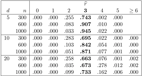
Xt3 is a random walk. None of them are stationary. The relative frequencies forbrtaking different
values are reported in Table 2. The boxplots of the estimation errors D1(A,A) are depicted inb
Figure 2 . The general pattern observed from the above stationary example (i.e. Example 1)
retains. The quality of our estimation improves when sample sizes increases. This is due to the
way in which the nonstationarity is specified in (4.1). For example, the sample{Xt2, t= 1,· · · , n} always consists of regular grid points on the segment of the liney = 3x between (0,0) and (1,3).
Therefore whennincreases, we obtain more information from the same (nonstationary) system.
Note that our method rests on the simple fact that the quadratic forms of the sample
cross-correlation function are close to 0 along the directions perpendicular to the factor loading space,
and are non-zero along the directions in the factor loading space. (See Remark 1(vi) and Remark
2(ii).) The departure from zero along the directions in the factor loading space in Example 2
is more pronounced than that in Example 1. This explains why the proposed method performs
better in Example 2 than in Example 1, especially whenn= 300 and 600.
Example 3. Figure 3 displays the monthly temperatures in the 7 cities in Eastern China in
January 1954 — December 1986. The cities concerned are Nanjing, Dongtai, Huoshan, Hefei,
Shanghai, Anqing and Hangzhou. The sample size n = 396 and d = 7. As well expected, the
data show strong periodic behaviour with period 12. We fit the data with factor models (2.1).
By setting p = 12, the estimated number of factors is br = 4. We applied principal components
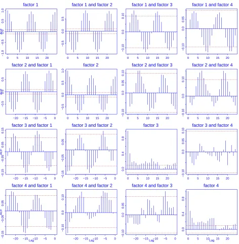
analysis to the estimated factors. The resulting 4 factors, in the descending order in terms of their
variances, are plotted in Figure 4, and their cross-correlation functions are displayed in Figure 5.
In fact the variances of the 4 factors are, respectively, 542.08, 1.29, 0.07 and 0.06. The first factor
accounts for over 99% of the total variation of the 4 factors, and 97.6% of the total variation of the
original 7 series. The periodic annual oscillation in the original data is predominately reflected
also by that of the second factor (the second panel in Figure 4). This suggests that the annual
temperature oscillation over this area may be seen as driven by one or at most two ‘common
factors’. The corresponding loading matrix is
b A=
.394 .386 .378 .387 .363 .376 .366
−.086 .225 −.640 −.271 .658 −.014 .164 .395 .0638 −.600 .346 −.494 −.074 .332 .687 −.585 −.032 −.306 .173 .206 −.139
τ , (4.2)
which indicates that the first factor is effectively the average temperatures over the 7 cities. The
residuals BbτY
t carries little dynamic information in the data; see the cross-correlation functions
depicted in Figure 6. The sample mean and sample covariance ofet are, respectively,
b
µe =
3.41
2.32
4.39
4.30
3.40
4.91
4.77
, Σbe=
1.56
1.26 1.05
1.71 1.34 1.91
1.90 1.49 2.10 2.33
1.37 1.16 1.46 1.58 1.37
1.67 1.26 1.91 2.09 1.37 1.97
[image:12.612.121.532.269.421.2]1.41 1.14 1.58 1.67 1.39 1.56 1.53 . (4.3)
Figure 5 indicates that the first two factors are dominated by periodic components with period
12. We estimated those components simply by taking the averages of all values in each of January,
February,· · · , December, leading to the estimated periodic components
(g1,1,· · · , g12,1) = (−1.61,1.33,11.74,28.06,41.88,54.51,63.77,62.14,49.48,33.74,18.29,3.50),
(g1,2,· · · , g12,2) = (1.67,1.21,0.47,0.17,0.41,0.48,1.37,2.13,2.98,3.05,2.78,2.22) (4.4)
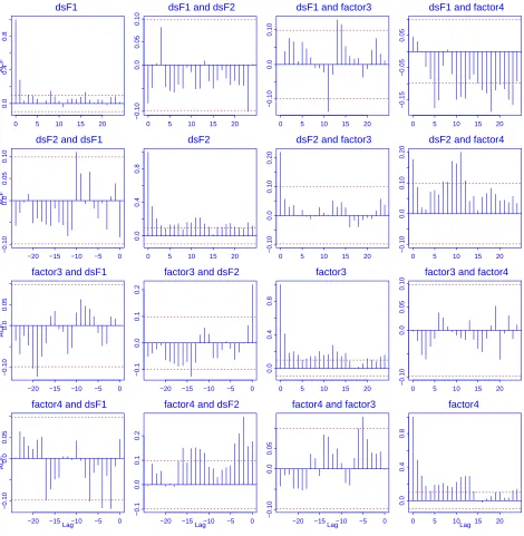
for, respectively, the first and the second factors. Figure 7 displays the cross-correlation functions
of the 4 factors after removing the periodic components from the first two factors. It shows that
the autocorrelation in each of those 4 series is not very strong, and furthermore cross correlation
among those 4 series (at non-zero lag) are weak. We fitted a vector autoregressive model to
Brockwell & Davis 1991) with the estimated coefficients:
b
ϕ0=
.07
−.02
−.11 .10
, Φb1=
.27 −.31 .72 .40
.01 .36 −.04 .04
.00 −.01 .42 −.02
−.00 .03 .03 .48
, (4.5)
b Σu =
14.24
−.17 .23
−.02 .03 .05 .042 .01 −.00 .05
. (4.6)
Both multivariate portmanteau tests (with the lag value p = 12) of Li & Mcleod (1981) and
Reinsel (1997, p.149) for the residuals from the above fitted vector AR(1) model are insignificant
at the 5% level. The univariate portmanteau test is insignificant at the level 5% for three (out of
the four) component residual series, and is insignificant at the level 1% for the other component
residual series. On the other hand, a vector AR(2) model was selected by the AIC for the 4 factor
series with vector AR(1) as its closest competitor. In fact the AIC values are, respectively, 240.03,
0.11, 0.00, 6.38 and 18.76 for the AR-order 0, 1, 2, 3 and 4.
Overall the fitted model for the month temperature vector Yt is
Yt=Abξt+et,
where the factor loading matrixAb is given in (4.2), the mean and covariance of white noiseetare
given in (4.3), and the 4×1 factorξt follows VAR(1) model
ξt−αt=ϕb0+Φb1(ξt−1−αt−1) +ut,
where the periodic component ατt = (gm(t),1, gm(t),2,0,0), gt,i is given in (4.4),
m(t) ={k1≤k≤12 and t= 12p+kfor some integerp≥0},
Acknowledgment
This project was partially supported by an EPSRC research grant. The authors thank
Profes-sor Valdimir Spokoiny for helpful discussion, Mr Da Huang for making available the temperature
data analyzed in Example 3. Thanks also go to two referees for their helpful comments and
suggestions.
Appendix
Proofs
We use the same notation as in section 3. We first introduce two lemmas concerning the
D-distance defined in (3.1) and condition C1. We then proceed to the proofs for Theorems 1
and 2.
Lemma 1. (i) It holds for anyH1,H2,H3 ∈ H that
D(H1,H3)≤D(H1,H2) +D(H2,H3).
(ii) For any H1,H2,Ψ(H1) = Ψ(H2) and Ψn(H1) = Ψn(H2)provided D(H1,H2) = 0.
Proof. (i) For any symmetric matrices M1,M2 and M3, it follows from the standard triangle
inequality for the matrix norm|| · || thatkM1−M3k ≤ kM1−M2k+kM2−M3k,that is q
tr(M2
1+M23−2M1M3)≤ q
tr(M2
1+M22−2M1M2) + q
tr(M2
2+M23−2M2M3). (A.1)
Let M1 = H1Hτ1, M2 = H2Hτ2 and M3 = H3Hτ3. Since now tr(M2i) = tr(Mi) = d−r for
i= 1,2,3. The inequality required follows from (A.1) and (3.1) directly.
(ii) Under the condition D(H1,H2) = 0, H1Hτ1 = H2Hτ2 as it is the projection matrix into
the linear spaceM(H1) =M(H2). Now
kHτ1ΣkH1 k2= tr{(H1τΣkH1)τHτ1ΣkH1}= tr(ΣτkH1Hτ1ΣkH1Hτ1) =kHτ2ΣkH2 k2 .
Hence Ψ(H1) = Ψ(H2). The equality for Ψn may be proved in the same manner.
Lemma 2. Let {Yt} be a ϕ-mixing process and ESk → Σk. Suppose that Yt can be
represented as Yt=Ut+Vt, whereUtand Vt are uncorrelated for each t,supt≥1EkUtkh <∞
for some constant h >2, and
1 n
n
X
t=1
Vt→P c,
1 n
n
X
t=1
wherec is a constant vector. It holds that
(i) Sk→Σk in probability, and
(ii)Sk →Σk almost surely provided that the mixing coefficients satisfy the condition
ϕ(m) =
O(m−2bb−2−δ), if1< b <2,
O(m−2b−δ), ifb≥2,
(A.3)
whereδ >0is a constant, and the convergence in condition (A.2) is also almost surely.
Proof. Assertion (i) follows from the the law of large number for ϕ-mixing processes; see,
eg.Theorem 8.1.1 of Lin & Lu (1997). Applying the result of Chen & Wu (1989) to the sequences
{Ut} and{UtUτt−i}, and using the condition (A.2), we may obtain (ii).
Proof of Theorem 1. Applying the Cauchy-Schwartz inequality to the matrix norm, we have
|Ψn(H)−Ψ(H)| ≤ p
X
k=1
kHτSkHk2− kHτΣkHk2
≤ p
X
k=1
kHτ(Sk−Σk)Hk[kHτSkHk+kHτΣkHk]≤kHk4 p
X
k=1
kSk−Σkk[kSk k+kΣkk].
Note that k H k2= d−r for any H ∈ H, kSk−Σkk → 0 in probability, which is implied by
condition C1, and kSkk+kΣk k=OP(1). Hence,
sup
H∈HD
|Ψn(H)−Ψ(H)|→P 0. (A.4)
Lemma 1(i) ensures that (HD, D) is a well-defined metric space which is complete. Lemma 1(ii)
guarantees that Ψn(·) is a well-defined stochastic process index by H ∈ HD, and Ψ(·) is
well-defined function on the metric space (HD, D). Now it follows from the argmax theorem (Theorem
3.2.2 and Corollary 3.2.3 of van der Vaart & Wellner 1996) thatD(Bb,B)→0 in probability. To show the convergence with probability 1, note that the convergence in (A.4) is with
prob-ability 1 provided Sk → Σk with probability 1. Suppose by contradiction that there exists a δ
such thatP{lim supn→∞D(Bb,B0)> δ}>0.Denote H′D =HD∩ {B:D(B, B0)≥δ}. Then H′D
is a compact subset ofHD. Note that supH∈HD|Ψn(H)−Ψ(H)|
a.s.
→ 0 implies that there exists a set of sample points Ω′ satisfying Ω′
⊂ {lim supn→∞D(Bb,B0) > δ} and P(Ω′)>0 such that for each ω ∈Ω′ one can find a subsequence
{Bbnk(ω)} ⊂ H ′
D with Bbnk(ω)→B∈ H ′
D.Then, by the
definition ofB,b
Ψ(B) = lim
holds forω ∈Ω′ and with positive probability. This is a contradiction to ConditionC
2. Therefore
it must hold that D(Bb,B0) → 0 with probability 1.
Proof of Theorem 2. Denote bys(i,j),k andσ(i,j),k, respectively, the (i, j)-th element ofSk and
Σk. By the Central Limit Theorem for ϕ-mixing processes (see Lin & Lu 1997, Davidson 1990),
it holds that √n{s(i,j),k −Es(i,j),k} →N(i,j),k in distribution, where N(i,j),k denotes a Gaussian
random variable, i, j= 1, ..., d. Hence,k√n(Sk−ESk)k=OP(1).It holds now that
sup
H∈HD
√
n|Ψn(H)−Ψ(H)| ≤ sup
H∈HD
√
n
p
X
k=1
kHτSkHk2 − kHτΣkHk2
≤ sup
H∈HD p
X
k=1
kHτ√n(Sk−ESk)Hk ·[kHτSkHk+kHτΣkHk]
+ sup
H∈HD p
X
k=1
kHτ{√n(ESk−Σk)}Hk ·[kHτSkHk+kHτΣkHk]
≤ p sup
H∈HD,1≤k≤p
kHτ√n(Sk−ESk)Hk ·[kHτSkHk+kHτΣkHk]
+p sup
H∈HD,1≤k≤p
kHτ{√n(ESk−Σk)}Hk ·[kHτSkHk+kHτΣkHk]
≤ p(d−r)4{ sup 1≤k≤pk
√
n(Sk−ESk)k ·[kSkk+kΣkk]
+ sup 1≤k≤pk
√
n(ESk−Σk)k]·[kSk k+kΣkk]} = OP(1). (A.5)
By condition C3, (A.5) and the definitions ofB and B, we have thatb
0 ≤ Ψn(B)−Ψn(B)b
= Ψ(B)−Ψ(B) +b OP(1/√n)≤ −a[D(Bb,B)]c+OP(1/√n).
Now let n→ ∞ in the above expression, it must hold that D(Bb,B) =OP(n− 1
2c).
References
Ahn, S.K. (1997). Inference of vector autoregressive models with cointegration and scalar com-ponents. Journal of the American Statistical Association,93, 350-356.
Anderson, T.G. & Lund, J. (1997). Estimating continuous time stochastic volatility models
of the short term interest rates. Journal of Econometrics,77, 343-377.
Anderson, T.W. (2002). Canonical correlation analysis and reduced rank regression in
Bai, J. & Ng, S. (2002). Determining the number of factors in approximate factor models.
Econometrica,70, 191-222.
Brillinger, D.R. (1981). Time Series Data Analysis and Theory, Extended edition,
Holden-Day, San Francisco.
Box, G. & Tiao, G. (1977). A canonical analysis of multiple time series. Biometrika, 64, 355-365.
Brockwell, J.P. & Davis, R.A. (1991). Time Series Theory and Methods (2nd Edition).
Springer, New York.
Chen, X. R. &Wu, Y. H. (1989). Strong law for a mixing sequence,Acta Math. Appl. Sinica.
5, 367-371.
Davidson, J. (1990). Central limit theorems for nonstationary mixing processes and near-epoch
dependent functions. Discussion Paper No. EM/90/216, Suntory-Toyota International Centre for Economics and Related Disciplines, London School of Economics, Houghton street, London WC2A 2AE.
Engle, R. & Watson, M. (1981). A one-factor multivariate time series model of metropolitan
wage rates. Journal of the American Statistical Association, 76, 774-781.
Forni, M., Hallin, M., Lippi, M. & Reichlin, L. (2000). The generalized dynamic factor
model: identification and estimation. Review of Econ. Statist. 82, 540-554.
Francq, C., Roy, R. & Zako¨ıan, J.-M. (2005). Diagnostic checking in ARMA models with
uncorrelated errors. Journal of the American Statistical Association,100, 532-544.
Geweke, J. (1977). The dynamic factor analysis of economic time series models. In “Latent
Variables in Socio-Economic Models”, eds. D.J. Aigner & A.S. Goldberger. North-Holland, Amsterdam, pp.365-383.
Geweke, J. & Singleton, K. (1981). Maximum likelihood confirmatory factor analysis of
economic time series. International Economic Review,22, 37-54.
Li, W.K. &Mcleod, A.I. (1981). Distribution of the residuals autocorrelations in multivariate ARMA time series models. Journal of the Royal Statistical Society, B,43, 231-239.
Lin, Z. & Lu, C. (1997). Limit Theory for Mixing Dependent Random Variables. Science Press/Kluwer Academic Publishers, New York/Beijing.
Ljung, G.M. & Box, G.E.P. (1978). On a measure of lack of fit in time series models.
Biometrika,65, 297-303.
Pe˜na, D. & Box, E.P. (1987). Identifying a simplifying structure in time series. Journal of the American Statistical Association,82, 836-843.
Pe˜na, D. &Poncela, P. (2006). Nonstationary dynamic factor analysis. Journal of Statistical Planning and Inference,136, 1237-1257.
Press, W.H., Teukolsky, S.A., Vetterling, W.T. & Flannery, B.P. (1992). Numerical
Priestley, M.B., Subba Rao, T. & Tong, H. (1974). Applications of principal component analysis and factor analysis in the identification of multivariate systems. IEEE Trans. Automt. Control,19, 703-704.
Reinsel, G.C. (1997). Elements of Multivariate Time Series Analysis, 2nd Edition. Springer,
New York.
Reinsel, G.C. & Velu, R.P. (1998). Multivariate Reduced Rank Regression. Springer, New
York.
Stock, J.H. & Watson, M.W. (2002). Forecasting using principal components from a large
number of predictors. Journal of the American Statistical Association, 97, 1167-1179.
Table 1: Relative frequencies for rbtaking different values in Example 1. (The true value of r is 3.)
b r
d n 0 1 2 3 4 5 ≥6
5 300 .000 .209 .444 .345 .002 .000
600 .000 .071 .286 .633 .010 .000 1000 .000 .004 .051 .933 .120 .000
10 300 .000 .219 .524 .255 .002 .000 .000
600 .000 .049 .290 .649 .012 .000 .000 1000 .000 .007 .062 .898 .033 .000 .000
20 300 .000 .162 .543 .285 .010 .000 .000
Table 2: Relative frequencies for rbtaking different values in Example 2. (The true value of r is 3.)
b r
d n 0 1 2 3 4 5 ≥6
5 300 .000 .000 .255 .743 .002 .000
600 .000 .000 .083 .907 .010 .000 1000 .000 .000 .033 .945 .022 .000
10 300 .000 .000 .283 .695 .022 .000 .000
600 .000 .000 .103 .842 .054 .001 .000 1000 .000 .000 .051 .871 .077 .001 .000
20 300 .000 .000 .258 .663 .076 .001 .002
0.0
0.2
0.4
0.6
0.8
n=300 n=600 n=1000
d=5
0.3
0.4
0.5
0.6
0.7
0.8
0.9
n=300 n=600 n=1000
d=10
0.80
0.85
0.90
0.95
n=300 n=600 n=1000
[image:21.612.82.522.42.248.2]d=20
0.0
0.1
0.2
0.3
0.4
n=300 n=600 n=1000
d=5
0.3
0.4
0.5
0.6
0.7
n=300 n=600 n=1000
d=10
0.75
0.80
0.85
0.90
n=300 n=600 n=1000
[image:22.612.80.525.43.249.2]d=20
• • • • •• ••• • • • • • • • • •• •• • • • •• • •• • • • • • • • • • • • • •• • • • • • •• • •• • • • • • • • •• • • • • • • • • • • •• • • • • •• • • • • •• • • • •• • • • • • • •• • • •• •• • • • •• • • • • • • • • • •
0 20 40 60 80 100 120
0 5 15 25 • •• • •• ••• • • • • • • • • •• •• • • • • • • •• • • • • • • • ••• • • •• • • • • • •• • • • • • • • • • • •• • • • • • • • • • • •• • • • • • • • • • • •• • • • • • • • • • • • •• • • • • • • • • • •• • • • • • • • • • •
0 20 40 60 80 100 120
0 5 15 25 •• • • •• •• • • • • • • • • • •• •• • • • •• • •• ••• • • • • • • • • • • • • • • • • •• • •• • • • • • • • •• • •• • • • • • • • •• •• • ••• • • • • •• • • • •• • • • • • • •• • • • • • • • • • •• •• •• • • • • • •
0 20 40 60 80 100 120
0 5 15 25 •• • • •• ••• • • • • • • • •• • • • • • • •• • •• ••• • • • • •• • • • •• • • • • • •• • •• ••• • • • • •• • • • • • • • • • • •• • • • •• •• • • • •• • • • •• • • • • • • •• • • •• • • • • • •• • • •• • • • • • •
0 20 40 60 80 100 120
0 10 20 30 • •• • •• •• • • • • • •• • • • • • • • • • • • • •• • • • • • • • • • • • • • • • • • • • •• • • • • • • • • • • • • • • • • • • • • • • •• •• • • • • • • • • • • • • • • • • • • • • • •• • • • • • • • • • •• • • •• • • • • • •
0 20 40 60 80 100 120
0 5 15 25 • • • • • •• • • • • •• • • • •• • • • • • • •• • •• • • • • • • • • • • • • •• • • • • • •• • •• • • • • • • • •• • • • • • • • • • • • • • • • •• •• • • • •• • • • • •• • • • • • •• • • •• •• • • • •• • • •• • • • • • •
0 20 40 60 80 100 120
0 5 15 25 • •• • •• •• • • • • • •• • • •• •• • • • •• • •• • • • • • • • • • • • • • • • • • • • •• • •• • • • • • • • •• • • • • • • • • • • •• •• • • • • • • • • • • • • • • • • • • • • • •• • • • • • • • • • •• • • •• • • • • • •
0 20 40 60 80 100 120
5
15
[image:23.612.66.540.36.617.2]25
• • • •• • • • • • • • •• • • • • • • • • • • •• • • • • •• • • • • • • • • • •• •• • • • • • • •• • •• • • • • • •• • ••• • • • • • •• • • • •• •• • • • • • • • • • • • • • • • • •• •• • • • • • • • • •• • • •• • • • • •
0 20 40 60 80 100 120
0 20 40 60 • • •• • •• • • •• • • • • • • •• • • • • • • • • • • • • • • • •• • • • •• • • • •• • • • • •• • • • • • • • ••• • • • • • • • • • • • • • • •• • ••• • • • • • •• • •• • ••• • • • •• • • • • • •••• • • • • • • • •• •
0 20 40 60 80 100 120
0 1 2 3 4 • • • • • • •• • • •• • • • • • • • • • • •• • •• • • •• • • • • •• • • • • • • • • • • • • • • • • • • • • • • • • • • • • • • • • • • • • • •• • • • • • • • • • • • • • • • • • •• • • • • • • • • • • • •• • • • • • • • • • • • •
0 20 40 60 80 100 120
−0.6 0.0 0.6 •• •• • • • • • • • • • • • ••• • • • • • • • • • • • •• • • •• • • • • • • • • • • • • • • • • • • • • • • • • • • • • • • • •• •• • • • • • •• • • •• •• • • • • • • • • • • • • • • • • •• • • • • • • • • • • • •• • • •• • •
0 20 40 60 80 100 120
−0.4
0.0
[image:24.612.68.537.193.523.2]0.4
factor 1
ACF
0 5 10 15 20
−1.0
−0.5
0.0
0.5
1.0
factor 1 and factor 2
0 5 10 15 20
−0.5
0.0
0.5
factor 1 and factor 3
0 5 10 15 20
−0.10
0.0
0.10
factor 1 and factor 4
0 5 10 15 20
−0.10
0.0
0.05
factor 2 and factor 1
ACF
−20 −15 −10 −5 0
−0.5
0.0
0.5
factor 2
0 5 10 15 20
−0.5
0.0
0.5
1.0
factor 2 and factor 3
0 5 10 15 20
−0.10
0.0
0.05
0.10
factor 2 and factor 4
0 5 10 15 20
−0.10
0.0
0.10
factor 3 and factor 1
ACF
−20 −15 −10 −5 0
−0.15
−0.05
0.05
0.15
factor 3 and factor 2
−20 −15 −10 −5 0
−0.15
−0.05
0.05
factor 3
0 5 10 15 20
0.0
0.4
0.8
factor 3 and factor 4
0 5 10 15 20
−0.10
0.0
0.05
0.10
factor 4 and factor 1
Lag
ACF
−20 −15 −10 −5 0
−0.15
−0.05
0.05
factor 4 and factor 2
Lag
−20 −15 −10 −5 0
−0.10
0.0
0.10
factor 4 and factor 3
Lag
−20 −15 −10 −5 0
−0.10
0.0
0.05
factor 4
Lag 0 5 10 15 20
0.0
0.4
[image:25.612.66.538.118.599.2]0.8
residual 1
ACF
0 5 10 15 20
0.0
0.2
0.4
0.6
0.8
1.0
residual 1 and residual 2
0 5 10 15 20
−0.10
−0.05
0.0
0.05
0.10
residual 1 and residual 3
0 5 10 15 20
−0.15
−0.05
0.05
residual 2 and residual 1
ACF
−20 −15 −10 −5 0
−0.10
0.0
0.05
0.10
residual 2
0 5 10 15 20
0.0
0.2
0.4
0.6
0.8
1.0
residual 2 and residual 3
0 5 10 15 20
−0.10
−0.05
0.0
0.05
0.10
residual 3 and residual 1
Lag
ACF
−20 −15 −10 −5 0
−0.10
−0.05
0.0
0.05
0.10
residual 3 and residual 2
Lag
−20 −15 −10 −5 0
−0.10
−0.05
0.0
0.05
0.10
residual 3
Lag
0 5 10 15 20
0.0
0.2
0.4
0.6
0.8
[image:26.612.143.460.186.528.2]1.0
dsF1
ACF
0 5 10 15 20
0.0
0.4
0.8
dsF1 and dsF2
0 5 10 15 20
−0.10
0.0
0.05
0.10
dsF1 and factor3
0 5 10 15 20
−0.10
0.0
0.10
dsF1 and factor4
0 5 10 15 20
−0.15
−0.05
0.05
dsF2 and dsF1
ACF
−20 −15 −10 −5 0
−0.10
0.0
0.05
0.10
dsF2
0 5 10 15 20
0.0
0.4
0.8
dsF2 and factor3
0 5 10 15 20
−0.10
0.0
0.10
0.20
dsF2 and factor4
0 5 10 15 20
−0.10
0.0
0.10
0.20
factor3 and dsF1
ACF
−20 −15 −10 −5 0
−0.10
0.0
0.05
factor3 and dsF2
−20 −15 −10 −5 0
−0.1
0.0
0.1
0.2
factor3
0 5 10 15 20
0.0
0.4
0.8
factor3 and factor4
0 5 10 15 20
−0.10
0.0
0.05
0.10
factor4 and dsF1
Lag
ACF
−20 −15 −10 −5 0
−0.10
0.0
0.05
factor4 and dsF2
Lag
−20 −15 −10 −5 0
−0.1
0.0
0.1
0.2
factor4 and factor3
Lag
−20 −15 −10 −5 0
−0.10
0.0
0.05
factor4
Lag 0 5 10 15 20
0.0
0.4
[image:27.612.67.537.114.595.2]0.8